Rock Physics

Dvorkin/RockPhysicsRockPhysicsJack P. Dvorkin

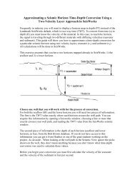
PrefaceDvorkin/RockPhysics 1Interpretation of Seismic Data. The main geophysical tool for illuminating thesubsurface is seismic. Seismic data yield a map of the elastic properties of thesubsurface. This map is useful as long as it can be interpreted to delineatestructures and, most important, quantify reservoir properties. Rock physicsprovides links between the sediment's elastic properties and its bulk properties(porosity, lithology) and conditions (pore pressure and pore fluid).What is Rational Rock Physics. Rock physics’ mission is to translate seismicobservables into reservoir properties, e.g., translate impedance into porosity. Thesimplest approach is to compile a laboratory data set, relevant to the site underinvestigation, where, e.g., impedance and porosity are measured on a set samples.The resulting impedance-porosity trend can be applied to seismic impedance tomap it into porosity. The applicability of an empirical trend is as good as the dataset it has been derived from. Extrapolation outside of the data set range is possibleonly if the physics is understood and theoretically generalized.MISSION OF ROCK PHYSICSSediment Elastic Properties(P-Impedance, Poisson’s Ratio)Sediment Bulk Properties(Porosity, Lithology, Permeability)andConditions (Fluid, Pressure)•Measure•Relate•UnderstandTransform FunctionFromRock PhysicsControlled Experimentk SwVp P VshVsφLABLOGS

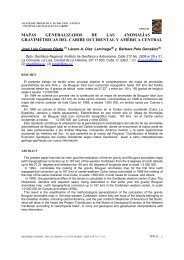
Methods of Rock PhysicsReflection and InversionDvorkin/RockPhysics 1Reflection amplitude carries information about elasticcontrast in the subsurface. Inversion attempts to translatethis information into elastic properties at a point in space.Point properties are important because we are interested inabsolute values of porosity and saturation at a point inspace.La Cira Norte. Courtesy Ecopetrol and Mario Gutierrez.

BasicsElasticityDvorkin/RockPhysics 1x 1Stress TensorStrain TensornTx 1ux 2x 2x 3T i= σ ijn jε ijx 3σ ij= σ jii ≠ j; ε ij= ε jii ≠ j.= 1 2 ( ∂u i∂x j+ ∂u j∂x i)Hooke's law: 21 independent constantsσ ij= c ijkle kl; c ijkl= c jikl= c ijlk= c jilk, c ijkl= c klij.Isotropic Hooke's law: 2 independent constants (elastic moduli)σ ij= λδ ijε αα+ 2µε ij; ε ij= [(1 + ν )σ ij− νδ ijσ αα]/E.λ and µ -- Lame's constants; ν -- Poisson's ratio; E -- Young's modulus.Bulk Modulus Compressional Modulus Young’s ModulusandPoisson’s RatioK = λ + 2µ / 3 M = λ + 2µE = µ(3λ + 2µ )/(λ + µ )ν = 0.5λ /(λ + µ )ZXYShearσ xz= 2µε xzε xx= ε yy= ε zz= ε xy= 0σ zz= Eε zzν = −ε xx/ ε zzσ xx= σ yy=σ xy= σ xz=σ yz= 0Youngσ zz= Mε zzσ yy= λε zz=[λ /(λ + 2µ )]σ zz=[ν /(1 − ν )]σ zzε xx= ε yy=ε xy= ε xz= ε yz= 0Compressional

BasicsDynamic and Static ElasticityDvorkin/RockPhysics 1WAVE EQUATIONε ~ 10 -7u(z)CompressionalExperimentAσ(z)dzσ(z+dz)zAdzρ«« u = A[σ(z + dz) − σ(z)] = Adz∂σ / ∂z ⇒ ρ∂ 2 u / ∂t 2 = ∂σ / ∂zσ = Mε = M∂u / ∂z ⇒ ∂ 2 u / ∂t 2 = (M / ρ)∂ 2 u / ∂z 2 ≡ V p2∂ 2 u / ∂z 2Dynamic definitions:V p= M / ρ = (K + 4G / 3)/ρ; V s= G / ρ;M = ρV p 2 ; G = ρV s 2 ; K = ρ(V p 2 − 4V s 2 / 3); λ = ρ(V p 2 − 2V s 2 )STATIC UNIAXIAL EXPERIMENTε ~ 10 -2 Courtesy Ali Mese70Sample 10156-5860Axial Stress (MPa)50403020Pc = 2000 psi = 14.1 MPaPc = 500 psi = 3.52 MPaPc = 0100RADIALAXIAL-0.005 0 0.005 0.01 0.015 0.02Strain

Velocity and SaturationGassmann’s EquationsDvorkin/RockPhysics 2In static (low-frequency) limit, pore fluid affectsonly the bulk modulus of rockGassmann's Equations -- Basis of Fluid SubstitutionBulk Modulus ofRock w/FluidBulk Modulus ofMineral PhaseK SatK s− K Sat=K DryK s− K Dry+Bulk Modulus ofDry RockK fφ(K s− K f)PorosityBulk Modulus ofPore FluidShear Modulus ofRock w/FluidG Sat= G DryShear Modulus ofDry RockThe bulk modulus of rock saturated with a fluid isrelated to the bulk modulus of the dry rock andvice versaK Sat= K sφK Dry− (1 + φ)K fK Dry/ K s+ K f(1 − φ)K f+ φK s− K fK Dry/ K sK Dry= K s1 − (1 − φ)K Sat/ K s− φK Sat/ K f1 + φ − φK s/ K f− K Sat/ K sVelocity depends on the elastic moduli and densityV p=V s=(K Sat+ 4 3 G Dry)/ρ SatG Dry/ ρ Satρ Sat= ρ Dry+ φρ Fluid> ρ Dry

Velocity and PorositySummary of TheoriesDvorkin/RockPhysics 3

Rock Physics Models: Velocity-PorosityWyllie et al. (1956) Time Average (Empirical)Recommended ParametersRock Type Vsolid (km/s)Sandstone 5.480 to 5.950Limestone 6.400 to 7.000Dolomite 7.000 to 7.925P-wave VelocityTotal Porosity1V p=φ + 1 − φV FluidV SolidSound SpeedIn Pore FluidP-wave Velocityin Solid PhaseRaymer et al. (1980) Equations (Empirical) V p= (1 − φ) 2 V Solid+ φV Fluid⇐ φ < 0.37Raymer’s equation is moreaccurate than Wyllie’s.Neither one of the twoshould be used to modelsoft slow sands.Examples of applyingWyllie’s and Raymer’sequation to sandstonelab dataVp (km/s)6543ConsolidatedSandsRaymerWyllieCLEANSANDSTONESSoft SlowSandsFastSands20 0.1 0.2 0.3 0.4PorosityVp Raymer Predicted (km/s)654SANDSTONESw/CLAY33 4 5 6Vp Measured (km/s)Han (1986) Equations for Consolidated Sandstones (Empirical, Ultrasonic Lab Measurements)Pressure Saturation Equations Comments40 MPa 100% Water Vp=6.08-8.06φ Vs=4.06-6.28φ Clean Rock40 MPa 100% Water Vp=5.59-6.93φ-2.18C Vs=3.52-4.91φ-1.89C Rock w/Clay30 MPa 100% Water Vp=5.55-6.96φ-2.18C Vs=3.47-4.84φ-1.87C Rock w/Clay20 MPa 100% Water Vp=5.49-6.94φ-2.17C Vs=3.39-4.73φ-1.81C Rock w/Clay10 MPa 100% Water Vp=5.39-7.08φ-2.13C Vs=3.29-4.73φ-1.74C Rock w/Clay5 MPa 100% Water Vp=5.26-7.08φ-2.02C Vs=3.16-4.77φ-1.64C Rock w/Clay40 MPa Room-Dry Vp=5.41-6.35φ-2.87C Vs=3.57-4.57φ-1.83C Rock w/ClayVp and Vs are in km/s; the total porosity φ is in fractions; volumetric clay contentin the whole rock (not in the solid phase) C is in fractions.

Tosaya (1982) Equations for Shaley Sandstones (Empirical, Ultrasonic Lab Measurements)Pressure Saturation Equations Comments40 MPa 100% Water Vp=5.8-8.6φ-2.4C Vs=3.7-6.3φ-2.1C Rock w/ClayVp and Vs are in km/s; the total porosity φ is in fractions; volumetric clay contentin the whole rock (not in the solid phase) C is in fractions.Eberhart-Phillips (1989) Equations for Shaley Sandstones (Empirical, Based on Han’s Data)100% WaterSaturationV p= 5.77 − 6.94φ − 1. 73 C + 0.446[P − exp(−16.7P)]V s= 3.70 − 4.94φ − 1.57 C + 0.361[P − exp(−16.7P)]Vp and Vs are in km/s; differential pressure P is in kilobars. 1 kb = 100 MPa.Nur’s (1998) Critical Porosity Concept (Heuristic)Solid-PhaseBulk ModulusTotal PorositySolid-PhaseShear ModulusCritical PorosityK Dry= K Solid(1 − φ / φ c) G Dry= G Solid(1 − φ / φ c)Dry-RockBulk ModulusDry-RockShear ModulusCritical Porosity of Various RocksSandstones 36% - 40%Limestones 36% - 40%Dolomites 36% - 40%Pumice 80%Chalks 55% - 65%Rock Salt 36% - 40%Cracked Igneous Rocks 3% - 6%Oceanic Basalts 20%Sintered Glass Beads 36% - 40%Glass Foam 85% - 90%Compressional Modulus (GPa)806040200CrackedIgneous RockswithPercolatingCracksPumicewithHoneycombStructure0 0.2 0.4 0.6 0.8 1PorosityElastic Modulus / Mineral Modulus10.80.60.40.20BasaltDolomiteFoamGlass BeadsLimestoneRock SaltClean Sandstone0 0.2 0.4 0.6 0.8 1Porosity/Critical PorosityExamples of using Critical Porosity Conceptto mimic lab data

Contact Cement Model (Theoretical)CoordinationNumberCement'sCritical Porosity CompressionalModulusCement'sShearModulusDry-RockBulk ModulusK Dry= n(1 − φ c )M c S n6G Dry= 3K Dry5Dry-RockShear Modulus+ 3n(1 − φ c )G c S τ20S n= A n(Λ n)α 2 + B n(Λ n)α + C n(Λ n), A n(Λ n) = −0.024153⋅Λ −1.3646 n,B n(Λ n) = 0.20405⋅Λ −0.89008 n, C n(Λ n) = 0.00024649 ⋅Λ −1.9864 n;S τ= A τ(Λ τ, ν s)α 2 + B τ(Λ τ, ν s)α + C τ(Λ τ, ν s),A τ(Λ τ, ν s) = −10 −2 ⋅(2.26ν 2 0.079νs+ 2.07ν s+ 2.3) ⋅Λ 2 s +0.1754ν −1.342 sτ,B τ(Λ τ, ν s) = (0.0573ν 2 0.0274νs+ 0.0937ν s+ 0.202) ⋅Λ 2 s +0.0529ν −0.8765 sτ,C τ(Λ τ, ν s) = 10 −4 ⋅(9.654ν 2 0.01867νs+ 4.945ν s+ 3.1) ⋅Λ 2 s +0.4011ν −1.8186 sτ;Λ n= 2G c(1 − ν s)(1 − ν c)/[πG s(1 − 2ν c)], Λ τ= G c/(πG s);α = [(2 / 3)(φ c− φ)/(1− φ c)] 0.5 ;ν c= 0.5(K c/ G c− 2/3)/(K c/ G c+ 1/3);ν s= 0.5(K s/ G s− 2/3)/(K s/ G s+ 1/3).Elastic ModulusContactCementModel0.30 0.35 0.40PorosityUncemented Sand Model or Modified Lower Hashin-Shtrikman (Theoretical)φ / φK Dry= [c+ 1 − φ / φ c] −1 − 4 K HM+ 4 3G HMK + 4 3G HM3 G , HMG Dry= [ φ / φ cG HM+ z + 1 − φ / φ c] −1 − z, z = G HMG + z6⎛⎜⎝9K HM+ 8G HMK HM+ 2G HMK HM= [ n2 (1 − φ c) 2 G 2 118π 2 (1 − ν) P] 3, G 2 HM= 5 − 4ν (1 − φ c) 2 G 2 15(2 − ν) [3n2 P]2π 2 (1 − ν) 2⎞⎟;⎠3.Elastic ModulusUncemented SandModel0.30 0.35 0.40PorosityIn the above equations, K stands for bulk modulus and G stands for shear modulus. ν isPoisson’s ratio. Subscript ”c” with a modulus means “cement” and subscript ”s” meansgrain material. φ is the total porosity, and φ c is critical porosity. P is differential pressure.All units have to be consistent.

Constant Cement Model (Theoretical)φ / φK dry= (bK b+ 4G b/3 +1 − φ / φ bK s+ 4G b/3 )−1 − 4G b/3,G dry= ( φ / φ bG b+ z + 1 − φ / φ bG s+ z )−1 − z, z = G b69K b+ 8G bK b+ 2G b.Elastic ModulusConstantCementModelφ b is porosity (smaller than φ c) at which contact cement trend turns into constantcement trend. Elastic moduli with subscript “b” are the moduli at porosity φ b.These moduli are calculated from the contact cement theory with φ = φ b.φ b0.30 0.35 0.40PorosityModel for Marine Sediments (Theoretical)60K Dry= [ (1 − φ)/(1− φ ) c+ (φ − φ )/(1− φ )c c] −1 − 4 K HM+ 4 43G HM 3G HM3 G , HMG Dry= [ (1 − φ)/(1− φ ) c+ (φ − φ )/(1− φ )c c] −1 − z,G HM+ zzz = G HM6⎛⎜⎝9K HM+ 8G HMK HM+ 2G HM⎞⎟; φ > φ c.⎠Depth (mbsf)80100120a0.5 0.55 0.6 0.65Neutron PorosityDataThis ModelSuspension1.5 1.6 1.7 1.8P-Wave Velocity (km/s)Consolidated Sand Model or Modified Upper Hashin-Shtrikman (Theoretical)φ / φK Dry= [ b+ 1 − φ / φ b] −1 − 4 K b+ 4 3G sK s+ 4 3G s3 G , sG Dry= [ φ / φ bG b+ z + 1 − φ / φ bG s+ z ]−1 − z,z = G s69K s+ 8G sK s+ 2G s.Elastic moduli with subscript “b” are the moduli at porosity φ b. These moduli canbe calculated from the contact cement theory with φ = φ b, or chosen at some initialpoint as suggested by data.Bulk Modulus (GPa)605040302010K sModified UpperHashin-Shtrikman(K Phi )b b00 0.1 0.2 0.3PorosityNon-Load-Bearing ClayModel (Theoretical)5DryClay < 35%No Clay3% < Clay < 18%All SamplesThe velocity (or elastic moduli) areplotted versus the load-bearing frameporosity φ F = φ t + C(1- φ clay ) instead oftotal porosity φ t . C is the volume of clayin rock, and φ clay is the internalporosity of clay.A scatter collapses onto a single trend(right frame).Vp (km/s)430 0.1 0.2 0.3Porosity18% < Clay < 37%0 0.1 0.2 0.3Porosity0 0.1 0.2 0.3Load-Bearing Frame Porosity

Examples: Velocity-PorosityP-WAVAE VELOCITY (km/s)432QuartzCementClayCementCORE DATASATURATEDContactCementNon-ContactCement0.2 0.3POROSITYElastic ModulusConstantCementFriableContactCement0.30 0.35 0.40PorosityInitialSandPackVp (km/s)3.53.0Friable2.5ConstantCementSortingContactCement#2#10.25 0.30 0.35 0.40Porosity35M-Modulus (GPa)3025201510FriableContactCementP-Impedance8765ContactCementEquationShear Modulus (GPa)1412Friable10864ContactCementUnconsolidatedShaleEquation 40.2 0.3 0.4Total Porosity200 0.1 0.2 0.3 0.4Porosity5Han CleanHan 3-8% ClayHan >18% Clay5Han CleanHan 3-8% ClayHan >18% ClayAcae_8Depth > 9.5 kftCaliper < 9.5Vp (km/s)Vp (km/s)44Acae_7Depth > 9.5 kftCaliper < 9.50.1 0.2Density-Porosity0.1 0.2Density-Porosity

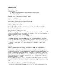
Velocity and PorosityFluvial Sandstones -- La Cira Case StudyDvorkin/RockPhysics 4Interpreting Impedance InversionSHALESANDCHANNELP-Wave Impedance11SHALE1098765SAND40 0.1 0.2 0.3Total PorosityALL DATA COURTESY ECOPETROL and MARIO GUTIERREZ

Vp and VsSummary of TheoriesDvorkin/RockPhysics 5

Dvorkin/RockPhysics 5Rock Physics Models: Vp and VsCastagna et al. (1985) Mudrock -- EmpiricalSand/Shale -- S W= 100%S-wave Velocity (km/s)P-wave Velocity (km/s)V S= 0.862 ⋅V P− 1.172Castagna et al. (1993) -- EmpiricalSand/Shale -- S W= 100%S-wave Velocity (km/s)P-wave Velocity (km/s)V S= 0.804 ⋅V P− 0.856Krief et al. (1990) -- “Critical Porosity’Any mineralAny fluid2V P_ Saturated2− V Fluid= V 2P_ Mineral2 2V S_SaturatedV S_ Mineral2− V FluidGrinberg/Castagna (1992)EmpiricalAny mineralS W= 100%S-wave Velocity (km/s)V S= 1 2 {[4∑ X i= 1i=14 2X ii=1 j =0∑P-wave Velocity (km/s)4jj∑ a ijV P] + [ ∑ X i( ∑ a ijV P) −1 ] −1 }i=12j =0i Mineral ai2 ai1 ai01 Sandstone 0 0.80416 -0.855882 Limestone -0.05508 1.01677 -1.030493 Dolomite 0 o.58321 -0.077754 Shale 0 0.76969 0.86735Willimas (1990) -- EmpiricalS W= 100%SandShaleS-wave Velocity (km/s)P-wave Velocity (km/s)V S= 0.846 ⋅ V P− 1.088V S= 0.784 ⋅ V P− 0.893