Hybrid mobility prediction of 802.11 infrastructur... - Computer ...

HYBRID MOBILITY PREDICTION OF 802.11 INFRASTRUCTURENODES BY LOCATION TRACKING AND DATA MININGBiju Issac 1 , Khairuddin Ab Hamid 2 , C.E. Tan 31,2 Faculty of EngineeringUniversity Malaysia Sarawak94300 Kota Samarahan, Sarawak, Malaysia1bissac@swinburne.edu.my, 2 khair@cans.unimas.my3 Faculty of CS and ITUniversity Malaysia Sarawak94300 Kota Samarahan, Sarawak, Malaysiacetan@fit.unimas.myAbstract - In an IEEE 802.11 Infrastructure network, as the mobile node is moving from one access pointto another, the resource allocation and smooth hand off may be a problem. If some reliable prediction isdone on mobile node’s next move, then resources can be allocated optimally as the mobile node movesaround. This would increase the performance throughput of wireless network. We plan to investigate ona hybrid mobility prediction scheme that uses location tracking and data mining to predict the futurepath of the mobile node. We also propose a secure version of the same scheme. Through simulation andanalysis, we present the prediction accuracy of our proposal.Keywords: Mobility prediction, mobility management, mobility patterns, location tracking, data mining.1. INTRODUCTIONThe mobility management in wireless networks covers the options for storing and updating the locationinformation of mobile users who are connected to the system. An interesting topic of research in mobilitymanagement field is mobility prediction. Mobility prediction can be explained as the prediction of a mobileuser‘s next movement where the mobile user is traveling between the nodes or access points of a wirelessnetwork. The predicted path or movement can help increase the efficiency of wireless network, by effectivelyallocating resources to the most probable access point (that can be the next point of attachment) instead ofblindly allocating excessive resources in the mobile nodes neighborhood of a mobile user (Saygin and Ulusoy,2002), (Gok and Ulusoy, 2000). This paper is organized as follows. Section 2 gives the details of existingmobility prediction schemes, along with location tracking and data mining. Section 3 shows the mobilityprediction proposal, section 4 is a secure version of that proposal, section 5 is simulation results and section 6 isthe conclusion.2. RELATED CONCEPTS AND WORKA mobility model should be made to capture the movements of real mobile nodes (MNs). Changes in speed anddirection of MN should happen in reasonable time slots. We discuss seven different mobility models forwireless networks (that are ad-hoc network oriented), which can as well be applied to infrastructure networks: Random Walk Mobility: A simple mobility model that is based on random directions and speeds. Random Waypoint Mobility: A model that includes pause times between changes in destination andspeed. Random Direction Mobility: A model that forces MNs to travel to the edge of the simulation area beforechanging direction and speed. A Boundless Simulation Area Mobility: A model that converts a two dimensional rectangular simulationarea into a torus-shaped simulation area. Gauss-Markov Mobility: A model that uses one tuning parameter or variable to vary the degree ofrandomness in the mobility pattern.

10 Journal of IT in Asia, Vol 3 (2010)Probabilistic Random Walk Mobility: A model that utilizes a set of probabilities to determine the nextposition of an MN.City Section Mobility: A simulation area that represents streets within a city.2.1 Random WalkMany entities in nature move in extremely unpredictable ways, and Random Walk Mobility was developed tomimic this erratic movement (Davies, 2000). By choosing a random direction and traveling speed, an MNmoves from its current position to a new position. The new speed and direction are both chosen from predefinedranges. If a mobile node reaches a simulation boundary, it ―bounces‖ off the simulation edge or borderwith an angle that is dependent on the incoming direction. The MN then continues along this new path. TheRandom Walk Mobility Model is a memory-less mobility pattern because it retains no knowledge concerning itspast locations and speed (Liang and Haas, 1999).2.2 Random WaypointThe Random Waypoint Mobility Model includes pause times between changes in direction and/or speed(Johnson and Maltz, 1996). A mobile node begins by pausing in one location for a certain period of time. Oncethis pause time finishes, the MN chooses a random destination in the simulation area and a speed that isuniformly distributed between a minimum and maximum value, [min_speed, max_speed]. The mobile node thentravels toward the new random destination at the speed that was selected. Upon its arrival, the mobile nodepauses for a specified time period before repeating the cycle. We note that the movement pattern of an MNusing the Random Waypoint Mobility Model is similar to the Random Walk Mobility Model if pause time iszero and [min_speed, max_speed] = [speed min , speed max ]. In most of the performance analysis that use theRandom Waypoint Mobility Model, the mobile nodes are distributed randomly. This initial random distributionof MNs has nothing to do with the manner in which nodes distribute themselves when moving.2.3 Random DirectionTo tackle the density waves in the average number of neighbours produced by the Random Waypoint MobilityModel, the Random Direction Mobility Model was created. A density wave is the clustering or grouping ofnodes in a specific part of the simulation area. In the case of the Random Waypoint Model, this clusteringoccurs near the center of the simulation area. In the Random Way Point Model, the probability of a mobile nodechoosing a new destination that is located in the center of the simulation area is quite high. Thus, the mobilenode path appears to converge and disperse again and again. In order to remove this strange behavior and toencourage a semi-constant number of neighbors throughout the simulation, the Random Direction MobilityModel was developed (Royer et al., 2001). In this model, mobile nodes choose a random direction in which totravel similar to the Random Walk Mobility Model. A mobile node then travels to the border of the simulationarea in that direction. Once the simulation boundary is reached, the MN pauses for a specified time, choosesanother angular direction (between 0 and 2π degrees) and continues the movement.2.4 A Boundless Simulation AreaIn the Boundless Simulation Area Mobility Model, there is a relationship between the previous direction oftravel and velocity of a mobile node with its current direction of travel and velocity (Hass, 1997). A velocityvector v = (v, θ) is used to describe an MN‘s velocity v as well as its direction θ; The MN‘s position isrepresented as (x, y). Both the velocity vector and the position are updated at every Δt time steps according tothe following formulas:v( t t) min[max( v(t) v,0),Vmax]; ( t t) ( t) ;x(t t) x(t) v(t)*cos ( t);y(t t) y(t) v(t)*sin ( t);(1)where V max is the maximum velocity defined in the simulation, Δv is the velocity change that is uniformlydistributed between [−A max ∗Δt, A max ∗Δt], A max is the maximum acceleration of a given MN, Δθ is the change indirection which is uniformly distributed between [−α ∗ Δt, α ∗Δt], and α is the maximum angular change in thedirection a mobile node is traveling. The Boundless Simulation Area Mobility Model is also different in how theboundary of a simulation area is dealt with. In all the mobility models discussed, MNs reflect off or stop movingonce they reach a simulation boundary or edge. In Boundless Simulation Area Mobility Model, MNs that reach

Hybrid Mobility Prediction of 802.11 Infrastructure Nodes by Location Tracking and Data Mining 11one side of the simulation area continue traveling and reappear on the opposite side of the simulation area. ThusMN can travel unhindered as this technique creates a torus-shaped simulation area.2.5 Gauss-MarkovThe Gauss-Markov Mobility Model was proposed to handle different levels of randomness through one tuningparameter. Initially each MN is assigned a current speed and direction. At fixed intervals of time – n, the speedand direction of each MN are changed and the mobile node moves. Specifically, the value of speed and directionat the n th instance is calculated based upon the value of speed and direction at the previous (n−1) st instance anda random variable using the following equations:sdnn s dn1n1 (1 )s (1 )d 2(1 ) sxn12(1 ) dxn1(2)where s n and d n are the new speed and direction of the MN at time interval n; α, where 0 ≤ α ≤ 1, is the tuningparameter used to vary the randomness; s and d are constants representing the mean value of speed and directionas n →∞; and s xn−1 and d xn−1 are random variables from a Gaussian distribution. Totally random values (orBrownian motion) are obtained by setting α = 0 and linear motion is obtained by setting α = 1 (Liang and Haas,1999). Intermediate levels of randomness are obtained by varying the value of α between 0 and 1. At each timeinterval the next location is calculated based on the current location, speed, and direction of movement.Specifically, at time interval n, an MN‘s position is given by the equations:xynn x yn1n1 s sn1n1cos dsin dn1n1(3)where (x n , y n ) and (x n−1 ,y n−1 ) are the x and y coordinates of the MN‘s position at the nth and (n−1) st timeintervals, respectively, and s n−1 and d n−1 are the speed and direction of the MN, respectively, at the (n−1) st timeinterval. To ensure that an MN does not remain near an edge of the grid for a long period of time, the MNs areforced away from an edge when they move within a certain distance of the edge. This is done by modifying themean direction variable d in the above direction equation.2.6 Probabilistic Random WalkChiang‘s mobility model uses a probability matrix to find the position of a particular MN in the next time step,which is denoted by three different states for position x and three different states for position y (Chiang, 1998).State 0, 1 and 2 are defined as follows: State 0 represents the current (x or y) position of a given MN, state 1represents the MN‘s previous (x or y) position, and state 2 represents the MN‘s next position if the MNcontinues to move in the same direction. The probability matrix used is:P(0,0)P P(1,0)P(2,0)P(0,1)P(1,1)P(2,1)P(0,2)P(1,2)P(2,2)where each entry P(c, d) represents the probability that an mobile node will go from state c to state d. The valueswithin this matrix are used for updates to both the MN‘s x and y position. In the simulator developed by Chiang,every node moves randomly with a predefined average speed. The following matrix contains the values Chiangused to calculate x and y movements: 0P1 0.30.30.50.700.500.72.7 City Section Mobility ModelIn the City Section Mobility Model, the simulation area imitates a street network that represents a portion of acity that has wireless network (Davies, 2000). The type of city being simulated dictates the streets and speedlimits on the streets.. For example, the streets may form a grid in the downtown area of the city with a highspeedhighway near the border of the simulation area to represent a loop around the city. Each MN begins the

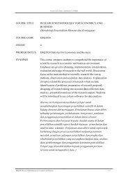
12 Journal of IT in Asia, Vol 3 (2010)simulation at a defined point on some street. An MN then randomly chooses a destination, also represented by apoint on some street. The movement algorithm from the current destination to the new destination locates a pathcorresponding to the shortest travel time between the two points; in addition, safe driving characteristics such asa speed limit and a minimum distance allowed between any two MNs exist. Upon reaching the destination, theMN pauses for a specified time and then randomly chooses another destination (i.e., a point on some street) andrepeats the process. The City Section Mobility Model provides realistic movements for a section of a city sinceit severely restricts the traveling behavior of MNs. In other words, all MNs must follow predefined paths andbehavior guidelines (e.g. traffic laws).2.8 Location Tracking and Data MiningLiu et al. (1998) have proposed a mobility modeling, location tracking, and trajectory prediction in WirelessATM Networks. This paper treats the problem by developing a hierarchical user mobility model that closelyrepresents the movement behavior of a mobile user, and that, when used with appropriate pattern matching andKalman filtering techniques, yields an accurate location prediction algorithm, which provides necessaryinformation for advance resource reservation (Liu et al., 1998). Capkun and collaborators (2001) propose adistributed, infrastructure-free positioning algorithm that does not rely on Global Positioning System (GPS). Thealgorithm uses the distances between the nodes to build a relative coordinate system in which the node positionsare computed in two dimensions (Capkun et al., 2001). Yavas and colleagues (2005) propose a new algorithmfor predicting the next inter-cell movement of a mobile user in a Personal Communication Systems network. Inthe first phase of the three phase algorithm, user mobility patterns are mined from the history of mobile usertrajectories. In the second phase, mobility rules are extracted from these patterns, and in the last phase, mobilitypredictions are accomplished by using these rules (Yavas et al., 2005).3. MOBILITY PREDICTION PROPOSALWe propose a centralized mobility prediction technique that is a hybrid version of location tracking without GPSand data mining technique called Location Tracking with Data mining Prediction Scheme (LTDPS). Locationtracking is done through a central server that receives the data regarding neighbouring APs from the mobilenode. Data mining is done by the same server by using the mobility path history of the mobile node movementsand by extracting the mobility patterns from that. We adapted some ideas from (Yavas et al., 2005), thoughimplemented it differently.R0 R1 R2 R3 R4 R50R01 213141R6 R7 R8 R9 R10 R1156 16117 819 1R12 R13 R14 R15 R16 R1710 111 112 13 14111R18 R19 R20 R21 R22 R2315 116 17 18 191111R24 R25 R26 R27 R28 R2920 121 R22 23 241R341R30 R31 R32 R33 R34 R35Figure 1. Access Points and Mobile regions arranged in a matrix format.One of the significant assumptions made is that the mobile node once it starts moving in one direction will notabruptly change its direction. The mobility model used is a modified Random Waypoint model (Johnson andMaltz, 1996), where the probability of choosing a center AP in the 5 x 5 grid, is not that high. Consider theaccess points numbered 0 to 24, arranged in a 5 x 5 matrix form. Surrounding each access point (AP) there arefour regions. These regions are numbered from R0 to R35 and is positioned around the 25 access points, as a 6 x

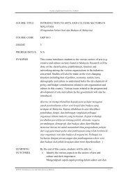
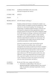
Hybrid Mobility Prediction of 802.11 Infrastructure Nodes by Location Tracking and Data Mining 136 matrix as shown in the Figure 1. The mobile node can move around any AP in the surrounding four regions orcan move to other adjacent regions of neighbouring AP.A Mobile Path Prediction Server (MPPS) is connected to the Local Area Network where the Access Points areconnected, to make the mobility prediction in a centralized way as shown in Figure 2.At frequent intervals of time, the mobile node transmits the Received Signal Strength Indication (RSSI) of thesurrounding APs to the MPPS. The IEEE 802.11 standard defines a way by which RF energy is to be measuredby the circuitry on a wireless network interface card (NIC). This value is an integer in the range of 0-255 (a 1-byte value) called the Receive Signal Strength Indicator (RSSI). None of the vendors have measured the 256different signal levels, and hence there is a standard discrepancy in that each vendor‘s 802.11 NIC will have aspecific maximum RSSI value called, ―RSSI_Max‖. For instance, Cisco chooses to measure 101 separate valuesfor RF energy, and their RSSI_Max is 100. Other companies such as Symbol uses an RSSI_Max value of 31 andAtheros chipset uses an RSSI_Max value of 60 (Wild Packets, 2002). Essentially the communication by MN toMPPS server involves the AP‘s identity and the received signal strength. The MN associates at any time withthe AP whose received signal strength is the highest.Mobile Path PredictionServer(along with RADIUSServer)LANAccessPoint 0AccessPoint 1Mobile NodeCloudAccessPoint 24Figure 2. Centralized Server for Mobility Prediction3.1 Location TrackingWe assume that the MN moves from one region to the other and pauses for a duration of t time units in anyregion, before making any movements further. By seeing the details of communication of AP‘s identity andRSSI value, the MPPS server is able to know which region the mobile node is located. All valid mobile paths bydifferent users or mobile nodes are recorded (along with regions) in a central database in MPPS server.Consider a section of the grid as shown in Figure 3. This is shown here for more clarity in our forthcomingdiscussions. For example, if the MN transmits details of AP numbered 0, 1, 5 and 6, MPPS server knows thatthe MN is located in region 7 (R7), according to Figure 1 and 3. Moreover, if the RSSI value (units) can be ofthe order as shown below: AP {0, 1, 5, 6} = RSSI {20, 30, 10, 5}, the MN is closer to AP1 and would beassociated to AP1 in region 7 (R7). So the mobile node path is: 1. It also shows that MN is also closer to AP0,compared to AP5 and AP6. After the starting AP, only when the MN is mobile, it transmits RSSI information.We call this information as RSSI sample. The MN is able to know it is mobile when the RSSI sample that itreceives from its neighbouring AP‘s differs widely. An error factor of ∆e can be allowed in RSSI valuesreceived by MN and transmitted to MPPS server. MN does the RSSI transmission to server in ∆t time unitsfrequency interval. By analyzing the RSSI sample, the MPPS server is able to know the direction of MNmovement. The region-AP map that the MPPS server stores can be shown in Table 1 for the first 12 regions,based on Figure 1.

14 Journal of IT in Asia, Vol 3 (2010)R0 R1 R2 R30R01 21R6 R7 R8 R956 16117R12 R13 R14 R15Figure 3. An enlarged view of a section of the grid shown in Figure 1.For example, if MN moves from region 7 and the RSSI sample transmitted can contain – RSSI {5, 38, 15, 25}corresponding to AP {0, 1, 5, 6}. This shows that MN is closer to AP1 and AP6 and is moving toward region 8.When it enters the region 8, the RSSI sample can be: RSSI {5, 10, 20, 35} corresponding to AP {1, 2, 6, 7}.When the RSSI sample received by MPPS server is quite similar in value or when current AP signal is weak, theMPPS server would send signals to reserve resources (as explained later) in AP7 (with highest RSSI value) andwould direct MN to initiate the handoff to AP7. If the handoff is successful, the mobile path is 1→7. Here theprediction would be accurate and the handover is initiated by the MPPS server.Location Tracking Algorithm:1. Initially MN is connected to an AP to start with, which would be located in Region Ri, where i=0 to 35. MNwould be tracking RSSI samples of all its neighboring AP‘s during t time intervals.2. The MN sends the RSSI samples (four highest values) to MPPS server, after its first connection is settled.MPPS server now knows the region where MN is located. The MN or the server knows that MN isstationary when the RSSI samples that it gets remain quite constant.Table 1. The region-AP map for location trackingNo. Region Neighbour APs1. 0 (corner) {0}2. 1 {0, 1}3. 2 {1, 2}4. 3 {2, 3}5. 4 {3, 4}6. 5 (corner) {5}7. 6 {0,5}8. 7 {0, 1, 5, 6}9. 8 {1, 2, 6, 7}10 9 {2, 3, 7, 8}11 10 {3, 4, 8, 9}12 11 {4, 9}3. When there is difference in RSSI samples received, the MN or server knows that MN is on the move andsends that changed RSSI samples to MPPS server. The MN movement can be within the same region, and itmay get connected to a closer AP whose RSSI value is highest, where the received RSSI samples would be{LV, LV, LV, HV} in any order. MPPS server checks the direction of MN movement, by analyzing theRSSI sample. At any time, if the RSSI value is as in Table 2, the MPPS server could sense MN‘s directionof movement and the process of resource reservation can be initiated by MPPS server.

Hybrid Mobility Prediction of 802.11 Infrastructure Nodes by Location Tracking and Data Mining 15Table 2. Location Tracking through RSSI samplesNo. RSSI Sample Direction/Position ofMobile Node1.2.3.{MV, MV, MV,MV}{LV, LV, HV,HV}{LV, LV, LV,HV}Middle of any RegionMovement toward thecenter of APs with HVvalues and horizontal orvertical cross overresults.Confirmed movementtoward the AP with HVvalue.4. MPPS server knows what would be the next region that MN would enter, based on RSSI sample value –whether high value (HV), medium value (MV) or low value (LV) as in Table 2. It immediately hasinformation to predict where the MN‘s next attachment AP would be, based on the following formula. If theMN moves from one region (current region) to the other region (next region), apply the formula: (CurrentAP {all neigbour APs}) ∩ Predicted Region {all APs} = {S}, where S is the set of probable next APs. If Scontains only one element, then that is the next predicted AP or if it contains 2 or more elements, MPPSserver does the prediction based on data mining to get the best possible path. Data mining concept isexplained in next section.As shown in Figure 4, the MN can move vertically, diagonally or horizontally (roughly, even though itdepends on the source point of traversal). This movement can be tracked by MPPS server. The RSSI valueswhich can be classified as low value (LV), medium value (MV) and high value (HV) is mapped on a 3 x 3matrix region within region 8, for MN connecting to AP6 from AP5, as in Figure 4.We understand that there could be RSSI noise, which may need filtering, such as Kalman, Gray or Fourierfiltering. But for the moment we are not considering the filtering options. There can be some indecisivescenarios. They are as follows – the RSSI values received are very weak or corrupted from all neighbouring APsand no clear decision can be taken on the next AP, the RSSI values received are similar in value, afteraccounting in the error factor of ∆e and the MN can still move. The RSSI values are classified equal or not bychecking whether it falls within a range of values (such as, 30-35 units) and not necessarily exact integer ordecimal values.Figure 4. Mobile Node (Dark circle) connected to AP5 in region 7 moves (vertically, diagonally or horizontally)and LV, MV and HV RSSI values in region 8.3.2 Data MiningTo counter the above indecisive scenarios, we incorporate the data mining approach in parallel, once MPPSserver knows the MN location, through RSSI samples sent. The Data mining approach consists of threephases: user mobility pattern mining, generation of mobility rules using the mined user mobility patterns, andthe mobility prediction. The next inter-cell movement of mobile users is predicted based on the mobility rules inthe last phase. For example, if the MN is in region 8 (R8), and connected to AP1, the only possible movementsare toward AP {2, 6, 7}. Using the extracted mobility patterns (for node movements: 1→2, 1→6, 1→7,

16 Journal of IT in Asia, Vol 3 (2010)1→2→7, 1→6→7) from the database of mobile paths in MPPS server, next AP prediction is done. If the RSSIsample received has similar values such as –RSSI {10, 12, 30, 30} for AP {1, 2, 6, 7}, then the MPPS servergoes in for data mining approach, as MN can still move. The values need not be 30 as listed for AP6 and AP7. Itcan be 30 and 35 and with an error factor of 5, the values are counted similar.3.2.1 User Mobility Pattern miningOnce the MPPS server knows the location of MN, it locates all the MN‘s immediate neighbours. Consider forexample a path: 19(22)→13(15)→8(9)→9(10)→4(4) →3(3), where values in parenthesis represent the regionswhere MN is present. The starting AP is AP19 and the region is 22. The MN moves to region 15 then and getsassociated to AP13. Once the MN moves from one region (current region) to the other region (next region), weneed to apply the formula: Current AP {all neigbhour APs} ∩ Next Region {all APs} = {S}, where S is the setof probable next APs. To find the predicted next AP, as per the rule given above, take the intersection ofneighbour AP set of AP19 and neighbour AP set of region 15. This is given as: AP19 {neigbours} ∩ R15 = {13,14, 18, 23, 24} ∩ {7, 8, 12, 13} ={13}. Thus the predicted next AP is 13, which is vaild as the MN movement.Predicted path = 19→13. From AP13 in region 15, the MN moves to region 9 and gets associated to AP8. AP13{neigbours} ∩ R9 ={7, 8, 12, 9, 14, 17, 18, 19}∩ {2, 3, 7, 8} = {7, 8}. Since we have 2 entries 7 and 8, we needto do pattern mining. From AP13, the MN can move to AP7 or AP8. So 13→7 and 13→8 patterns are searchedin the sorted database and their frequency count is noted as in Table 3. The path 13→8 is selected because ofhigher frequency count. AP8 is the next predicted AP. Predicted path = 13→7→8. This procedure is repeatedfor other nodes.Consider a path 22(26)→21(25)→15(18)→16(19). Following our earlier calculation, AP22{neigbours} ∩R25 ={16, 17, 18, 21, 23} ∩ {15, 16, 20, 21} ={20, 21}. Here MN moves from AP22 in region 26 to AP21 inregion 25, as 22→21 has higher frequency count (of 272) than 22→16 (where the count was 162), like wediscussed before. Predicted path is vaild and thus is: 22→21.Then it moves to region 18. So, AP21{neigbours} ∩ R28 ={15, 16, 17, 20, 22} ∩ {10, 15} ={15}. So theMN moves to AP15 in region 18. Predicted path is vaild and thus is: 22→21→15. From there it moves to region19. Following our earlier calculation again, AP15{neigbours} ∩ R19 ={10, 11, 16, 20, 21} ∩ {10, 11, 15, 16}={10, 11, 16}.Table 3. Mobility Pattern mining for 2 neighboursNo. Path Frequency1 13→7 2382 13→8 367Note there are there possible movements here, which are 15→10, 15→11 and 15→16. In such a situation,we would like to do the data mining, slightly differently [12] as in Table 4. The final score for 15→10 = 707 +x1*0.5 + x2*0.5, for 15→11 = 40 + x3*0.5 + x4*0.5 and for 15→16 = 54 + x5*0.5 + x6*0.5. Here, we aretaking a corruption factor of 0.5 that has to be multiplied with the ‗indirect path counts‘. When we consider thepath 15→10, paths such as 15→11→10 and 15→16→10 are termed as indirect paths, as they have the sourceand destination APs as vaild. Total score = score of 2 AP link + corruption factor * {sum of scores of 3 APlink}. In this case, we found our prediction not vaild (to be from 15→10, instead of the vaild path 15→16). Butthe concept will definitely work for other cases as the mobile path database gets populated.Table 4. Mobility Pattern mining for 3 neigboursNo. Path Frequency1 15→10 7072 15→11→10 x13 15→16→10 x24 15→11 405 15→10→11 x36 15→16→11 x47 15→16 548 15→10→16 x59 15→11→16 x6

Hybrid Mobility Prediction of 802.11 Infrastructure Nodes by Location Tracking and Data Mining 173.2.2 Generation of Mobility RulesAn example of mobility rule generation from our previous examples is given in Table 5. Mobility rule can thusbe generated as in Table 5, after the mining is done for specific paths. These mobility rules differ depending onthe direction of MN movement. Since we incorporate the concept of region, once a MN enters a region, it getsassociated to one of the neighbouring APs, depending on the direction of node movement. That narrows downthe probability of error as the movement can happen to 1, 2 or 3 APs, depending on which region MN is located.Table 5. Mobility rule generationNo. Region Movement Predicted Path1 AP13:R15→R9 AP8 (valid)2 AP22:R26→R25 AP21 (valid)3 AP15:R18→R19 AP10 (invalid)3.2.3 Prediction of MobilityOnce the Mobility rules are generated, the predicted next AP is the one whose path has the highest frequency. Inthe example that we are discussing, based on Table 5, the next predicted AP would be AP8, as per the first rulein Table 5. The MPPS server would send signals to reserve resources in AP8 and would allow MN to initiate thehandoff to AP8. To optimize the performance, in case of invalid prediction, the two highest frequencies can benoted and resources can be reserved on two APs. We haven‘t considered that option in our simulation.3.3 Overall Mobility Prediction AlgorithmThe overall mobility prediction algorithm is stated below that includes location tracking and data mining.1. Initially the Mobile Node (MN) starts by associating with a random Access Point (AP).2. The MN transmits the RSSI value received and the surrounding AP‘s identity (maximum of 4) to MPPSServer. MN stays with that AP for t time units, where t is variable. To be precise, MN sends a packet with value to Serverfor all the surrounding APs, where RSSI_NextAP and RSSI_CurrentAP is the RSSI values ofneighbouring AP and currently attached AP to MN respectively. As each region can have maximum 4APs and minimum 2 (or 1) APs, the right AP identity is ensured by checking the RSSI value. Thistransmission happens in regular intervals; for example, ∆t seconds/time units.3. For a given MN identity, the server would choose four packets with the highest RSSI values (for NextAP) and note the AP identity (even if the RSSI values match). In the four RSSI values selected, if all thevalues are above the Next AP RSSI threshold value (―region threshold‖ RSSI value, RSSI region_threshold ),then the MN is in the inner region with four neighbouring APs, or if only two values are above the NextAP RSSI threshold value, then the MN is in the outer region with two neighbouring APs, or if only onevalue is above the Next AP RSSI threshold value, then the MN is in the corner region with only oneneighbouring AP. Thus, analyzing the Next AP RSSI values by the Server would indicate to which APthe MN is getting closer. If one of the RSSI value is highest then the MN is closer to the correspondingAP, or if two of the highest RSSI values (or block values) are the same, then the MN is equally closer tothose two APs, or if three or four of the RSSI values are the same, then the MN is in the center of a givenregion.4. After t time units, the MN starts moving and it transmits RSSI sample to MPPS Server. Now the directionof movement of MN can be known to MPPS server, through the RSSI sample values that it receives after∆t time units, as explained before. If "n" packets sent by MN are same (having RSSI values same orcloser values), then the server knows that MN is stationary or moving closer to a specific AP for a periodof time.5. The MPPS server adopts data mining (that happens in parallel) to predict the next AP of MN attachment,when the RSSI sample values received in a set are similar (such as, for two or more APs) or when theRSSI samples is weak or no signals are coming from neigbouring APs. Here it uses the mobile node‘spast history to extract mobility patterns, whereby it can come to a good judgment, as explained in section

18 Journal of IT in Asia, Vol 3 (2010)3.2. Once the MN moves from one region (current region) to the other region (next region), we need toapply the formula: Current AP {all neighbor APs} ∩ Next Region {all APs} = {S}, where S is the set ofprobable next APs. If S contains only one element, then that is the next predicted AP or if it contains 2 ormore elements, it adopts data mining to get the best possible path.6. The MPPS server intimates the selected AP (selected with high RSSI value or selected through datamining) at an optimum hand-off time (t opt_handoff ), that a particular MN is trying to attach to it and informsabout the resources needed to be reserved, which is the first-stage reservation. A copy of this notice issent to MN also, optionally. In the next ∆t time units, if the MN senses that the Next AP RSSI value isequal to or greater than the threshold RSSI value (RSSI region_threshold ), the MN sends a second-stagereservation to the AP, according to the type of traffic like data, voice and video. The voice and videowould imply more buffer space in the second stage reservation request, unlike data that needs fewerbuffers.7. Hand off can be initiated through RSSI sample comparison or data mining. If the MN senses that theNext AP RSSI value is equal to or greater than the region threshold RSSI value (RSSI region_threshold ) and atthe same time, the current AP RSSI value is diminishing, hand off can be initiated from Current AP toNext AP through MPPS server. During the hand-off, the current AP‘s permission is sought to allow MNto get connected to Next AP.8. Once the handoff is successful, the mobile node path is stored in the MPPS database.Note: If the MN at any point is sensing that it is losing the network connection from the current AP, because ofsome delay in the communication from MPPS server, the MN can initiate the hand off to the new AP. This iscan be a backup option.4. SECURE MOBILITY PREDICTIONWe also propose a secure version of the above algorithm using a shared secret key, as the process is prone tomessage modification, spoofing and replay attacks by rouge mobile nodes. Message modification and spoofingattack happens when the attacker modifies the content (RSSI value or others) and identity of the AP or MNrespectively. Replay attack occurs when the attacker replays the captured packet at a later time for defeating theprediction or for masquerading. The secure mobility prediction packet exchange can be as follows:For RSSI Communication initiated by MN:1. The packet send by MN is appended by a message integrity control (MIC). The MN encrypts thepacket/message using 3DES with cipher block chaining (CBC). It cuts the message into predeterminedsizedof i blocks (where i = 1, 2, … n). It then uses the CBC residue (that is the last block output by CBCprocess) as the MIC (as MIC 1 , MIC 2 etc.), which would act as the checksum. The clear text message plusthe MIC would be transmitted to the server.2. The server encrypts the received plaintext message from MN using 3DES with the shared secret key (K SA )and performs the hashing process to produce a similar MIC (such as, MIC*). The server then checks if theMIC (received from MN) = MIC*, and if that‘s true, then the message is non-tampered in transit.Otherwise, it is rejected.3. Finally, the server sends an acknowledgement (ACK) and a random number (RND) or a nonce (as RND 1 ,RND 2 etc.) that is encrypted with the shared secret key K SA , i.e. (ACK+RND)K SA to MN.5. The MN verifies the encrypted ACK from server and the next message to MPPS server (after t time units)is similar to the initial communication, but with the addition of encrypted RND or nonce. If the server orMN at any time receives any unauthorized message, an alarm can be generated or logged and connectionrefused for that attempt. When the server responds back to MN with an (ACK+RND)K SA, it would be with adifferent RND or nonce.For Communication initiated by the MPPS server:6. If the MPPS server needs to communicate a message to MN in relation to resource reservation or handoff,the same approach can be done in the reverse order.

Hybrid Mobility Prediction of 802.11 Infrastructure Nodes by Location Tracking and Data Mining 19The packet exchange described above (initiated by MN) that can stop the security attacks is shown below for thetwo sets of interactions, as a set of equations:1. MN → MPPS : Message 1 + MIC 12. MPPS → MN : (ACK+RND 1 )K SA3. MN → MPPS : Message 2 + (RND 1 )K SA + MIC 24. MPPS → MN : (ACK+RND 2 ) K SAIf MPPS server needs to send a message to MN (i.e. initiated by server), it can be as follows:1. MPPS → MN : Message + (RND)K SA + MIC2. MN → MPPS : (ACK+RND)K SAAs we can observe, the security process involve only light encryption for authentication purposes and anadditional acknowledgement as overhead. The actual messages are sent as plain text to reduce processingoverhead.5. SIMULATION RESULTSThe simulation is done with the following parameters. A modified version of Random Waypoint Mobility modelis used, where nodes moves equally to the sides and center. The mobile node travels in a 6 x 6 region matrixwhich contains 5 x 5 access point matrix. Thus the 36 regions have 25 access points placed in a matrix format asshown in Figure 1.The simulation is run to create 10,000 mobile paths and this is stored in a central database of MPPS server.This data set is used for data mining and to create the mobility patterns. Later, a test set of 10 random mobilepaths were created (with a maximum of six access points and a minimum of three access points) and tested forprediction accuracy. The reasoning between the number of paths and the number of access points within them isthat there would be a minimum of thirty mobile node transitions from one access point to another (36transitions, as per Table 6) that would happen, which would make our calculations statistically significant. Theaccuracy of prediction through RSSI sample approach and location tracking is 100%, if the RSSI value receivedby MN is high from a particular AP, during its mobile path. The data mining approach which was done inparallel was simulated and the prediction analysis is as given below.Figure 5. Mobile Node Paths generated (only a sample of around 30 paths is shown).We would like to show the prediction accuracy for a sample of 10 paths, as given below. The mobile nodemovement history consisted of 10,000 mobile paths.Path 1: 7(8) →2(2) → 6(7) →1(1)Path 2: 13(15) → 7(8) → 1(1) → 0(0) → 6(7)Path 3: 23(27) → 17(20) →16(19) →11(13)→ 6(7)Path 4: 22(26) → 21(25) → 15(18) → 16(19)Path 5: 11(13) → 5(6) → 0(0)Path 6: 14(16) → 9(10) → 8(9) → 2(2) →1(1) → 0(0)

20 Journal of IT in Asia, Vol 3 (2010)Path 7: 17(20) → 12(14) → 6(7) →11(13)Path 8: 12(14) → 11(13) → 5(6) → 6(7)Path 9: 8(9) → 7(8) → 2(2) → 1(1) → 0(0)Path 10: 19(22) → 13(15) → 8(9) → 9(10) →4(4)→3(3)The values in the parenthesis are the region numbers. i.e. 7(8) means AP7 in region 8. As a result of thesimulation, the Table 6, 7 and 8 shows the prediction accuracy for the random sample considered above, usingthree different prediction schemes. The average accuracy of LTDPS was 76.4%. The predicted path contains,for example entries such as 0(1, 2) in row 1 of Table 6. The 0 is the predicted next AP (AP0) and inside theparenthesis, 1 is the actual node to which MN moved and 2 is the frequency rank of the predicted node, which isAP0. The variance between 33% (smallest value) and 100% (highest value) in Table 6 is the result of invalidprediction in the paths.Table 6. Predicted Path Accuracy Table for a sample using our prediction scheme (LTDPS)No Original Path Predicted PathAccuracy(%)1.7→2→6→17→1(2, 2)→6→0(1, 2)1 (33%)2.13→7→1→0→613→7→1→0→5(6, 2)3 (75%)3.23→17→16→11→623→17→16→11→ 5(6, 2)3 (75%)4.22→21→15→1622→21→15→10(16, 2)2 (67%)5.11→5→011→5→02 (100%)6.14→9→8→2→1→014→9→8→2→1→05 (100%)7.17→12→6→1117→11(12, 2)→6→112 (67%)8.12→11→5→612→11→5→ 0(6, 2)2 (67%)9.8→7→2→1→08→7→2→1→04 (100%)10.19→13→8→9→4→319→13→8→3(9, 2)→4→35 (80%)We compared our prediction method with two other methods, as baseline schemes. Refer to Tables 7 and 8.The first prediction method is called Mobility Prediction based on Transition Matrix (TM). In this method, acell-to-cell transition matrix is formed by considering the previous inter-cell movements of the mobile nodes orusers. The predictions are based on this transition matrix by selecting the x most likely cells or regions as thepredicted cells. We used TM for performance comparison because it makes predictions based on the previousmovements of the mobile node or user (Rajagopal et al., 2002). Assuming x=1 (as the previous scheme alsoused x=1), the average accuracy of TM was found to be 38.8% in our simulation.The second prediction method is the Ignorant Prediction (IP) scheme (Bhattacharya and Das, 2002). Thisapproach disregards the information available from movement history. To predict the next inter-cell movementof a user, this method assigns equal transition probabilities to the neighboring cells of the mobile nodescurrently residence cell. It means that prediction is performed by randomly selecting m neighboring cells of thecurrent cell. We have taken m to be the maximum no. of neighbours possible. The value in the parenthesis in thepaths shows the corrected AP number. The average accuracy of this scheme was found to be 36.3% and asexpected was quite inconsistent.

Hybrid Mobility Prediction of 802.11 Infrastructure Nodes by Location Tracking and Data Mining 21Table 7. Predicted Path Accuracy Table for a sample using Transition Matrix (TM) PredictionNo Original Path Predicted PathAccuracy(%)1.2.3.4.5.6.7.8.9.10.7→2→6→113→7→1→0→623→17→16→11→622→21→15→1611→5→014→9→8→2→1→017→12→6→1112→11→5→68→7→2→1→019→13→8→9→4→37→2→1(6,4)→5(1,2)13→8(7,3)→2(1,2)→0→5(6,2)23→22(17,3)→16→15(11,2)→10(6,3)22→21→20(15,2)→10(16,3)11→10(5,2)→014→9→14(8,3)→3(2,2)→1→017→16(12,3)→11(6,3)→5(1,3)12→11→5→ 0(6,5)8→3(7,3)→2→1→019→14(13,8)→8→3(9,5)→ 14(4,2)→9(3,2)1 (33%)1 (25%)1 (25%)1 (33%)1 (50%)3 (60%)0 (0%)2 (67%)3 (75%)1 (20%)Table 8. Predicted Path Accuracy Table for a sample using Ignorant PredictionNo Original Path Predicted PathAccuracy(%)1.2.3.4.5.6.7.8.9.10.7→2→6→113→7→1→0→623→17→16→11→622→21→15→1611→5→014→9→8→2→1→017→12→6→1112→11→5→68→7→2→1→019→13→8→9→4→37→1 (2)→1(6)→0(1)13→7→1→0→1(6)23→17→11(16)→10(11)→5(6)22→21→15→20(16)11→10(5)→014→8(9)→3(8)→3(2)→1→017→13(12)→7(6)→0(11)12→7(11)→5→0(6)8→2(7)→1(2)→7(1)→019→13→7(8)→2(9)→3(4)→30 (0%)3 (75%)1 (25%)2 (75%)1 (50%)2 (40%)0 (0%)1 (33%)1 (25%)2 (40%)A comparison bar graph that shows the prediction accuracy can be as shown in Figure 6, for the three differentschemes. It is very clear that LTDPS (our proposal) is having better accuracy and generally the accuracy of TMand IP tends to be lower.The dividing of surrounding AP area into four regions plays a great role in making the proposal moreaccurate. This would reduce the number of possible next AP set and hence the prediction can be more accurate.If such a division is not made, then based on the network model used in Figure 1, there would be eightneighbours to an AP, and to predict one of them would be quite a difficult task. So the location tracking throughRSSI samples, coupled with data mining makes our proposal work better. Note the higher bars that touch 100%a few times with LTDPS.Another observation that can be made is the frequency rank of the nodes (shown in brackets) in the predictedpath for LTDPS and TM from Table 6 and 7. From Table 6 for LTDPS, it is clear that the frequency rank ismostly 1 or 2. Frequency rank 1 means prediction is vaild (hence not shown in brackets in the Table). But fromTable 7 for TM, the frequency ranks fluctuates between 1, 2, 3, 4 and 5, thus showing how it‘s lacking inaccuracy. The maximum frequency deviation graphs for LTDPS and TM schemes can be as shown in Figure 7.

22 Journal of IT in Asia, Vol 3 (2010)Figure 6. Prediction accuracy graph for 10 random sample paths for LTDPS, TM and IP SchemesAs per Figure 7, a curve or line closer to frequency rank 1 is better. TM does not touch the frequency rank of1, as we are taking the maximum frequency deviation for all samples and in all paths at least one prediction isinvalid. The line or curve would touch frequency rank 1 if and only if all the predicted paths are valid. Forexample, a frequency rank of 2 shows that, though it has missed the right AP prediction, it has chosen the APthat has the next highest frequency rank. Sample paths 5, 6 and 9 shows for LTDPS that all the paths predictedare valid.Figure 7. Max. Frequency Deviation graph for 10 random sample paths for LTDPS and TM Schemes.Frequency rank 1 shows accurate prediction.Figure 8. Error graph for 10 random sample paths for LTDPS, TM and IP Schemes.Finally a curve plot of error margin of the three prediction schemes can be as shown in Figure 8. Here wedon‘t consider the number of AP transitions by the MN, but only the path errors in prediction. The closer, theline or curve is to the x-axis, the better the scheme is.

Hybrid Mobility Prediction of 802.11 Infrastructure Nodes by Location Tracking and Data Mining 236. CONCLUSIONThis paper presents a centralized novel mobility prediction scheme which combines mobile node‘s locationtracking through the analysis of RSSI samples and data mining through mobile nodes past movement history.The scheme works well with higher accuracy and low fluctuations with respect to frequency ranks. Typically,the movement history should be bigger for better prediction accuracy. Location tracking and data miningoperates in parallel and is used when they are needed for prediction. The prediction accuracy of locationtracking and data mining prediction scheme (LTDPS) looks quite satisfactory through our simulation analysis,as we compared its performance with other baseline schemes.ACKNOWLEDGMENTThis paper is an extended version of the paper submitted for CITA 2007 Conference, entitled –―A NovelMobility Prediction in 802.11 Infrastructure Networks by Location Tracking and Data Mining‖, held during July2007 in Kuching, Malaysia.REFERENCESBhattacharya, A., and Das, S.K. 2002. LeZi—Update: an information-theoretic approach to track mobile usersin PCS networks, ACM Wireless Networks, pp. 121-135.Capkun, S., Hamdi, M. and Hubaux, J., 2001. GPS-free positioning in mobile Ad-Hoc networks. In Proceedingsof the 34th Hawaii International Conference on System Sciences, Hawaii: USA.Chiang, C., 1998. Wireless Network Multicasting. PhD. University of California, Los Angeles.Davies, V., 2000. Evaluating mobility models within an ad hoc network. Master‘s thesis, Colorado School ofMines.Gok, G., and Ulusoy, O., 2000. Transmission of continuous query results in mobile computing systems.Information. Science, pp.37–63.Haas, Z., 1997. A new routing protocol for reconfigurable wireless networks, In Proceedings of the IEEEInternational Conference on Universal Personal Communications (ICUPC 1997), San Diego: USAJohnson, D. and D. Maltz, D., 1996. Dynamic source routing in ad hoc wireless networks, Mobile Computing,pp. 153–181.Liang B., and Haas, Z., 1999. Predictive distance-based mobility management for PCS networks. InProceedings of the Joint Conference of the IEEE Computer and Communications Societies (INFOCOM1999), New York: USA.Liang, B. and Haas, Z., 1999. Predictive distance-based mobility management for PCS networks, InProceedings of the Joint Conference of the IEEE Computer and Communications Societies (INFOCOM1999). New York: USALiu, T., Bahl, P. and Chlamtac, I., 1998. Mobility Modeling, Location Tracking, and Trajectory Prediction inWireless ATM Networks. IEEE Journal on Selected Areas in Communications, pp. 922-235.Rajagopal, S. Srinivasan, R.B, Narayan, R.B. and Petit, X.B.C, 2002. GPS-based predictive resource allocationin cellural networks. In Proceedings of the IEEE International Conference on Networks (ICON 2002),Sriperumbudur: IndiaRoyer, E., Melliar-Smith, P. M. and Moser, L., 2001. An analysis of the optimum node density for ad hocnetworks In Proceedings of the IEEE International Conference on Communications (ICC 2001).Helsinki: FinlandSaygin, Y. and Ulusoy, O., 2002. Exploiting data mining techniques for broadcasting data in mobile computingenvironments. IEEE Transactions on Knowledge Data Engineering, pp. 1387–1399.

24 Journal of IT in Asia, Vol 3 (2010)Wild Packets, 2002. Converting Signal Strength Percentage to dBm Values, Available at: [Accessed 17March 2008].Yavas, G., Katsaros, D., Ulusoy, O and Manolopoulos, Y., 2005. A data mining approach for locationprediction in mobile environments, Data & Knowledge Engineering, pp. 121–146.