Newton's Prism Experiment and Goethe's Objections
Newton's Prism Experiment and Goethe's Objections
Newton's Prism Experiment and Goethe's Objections

Create successful ePaper yourself
Turn your PDF publications into a flip-book with our unique Google optimized e-Paper software.
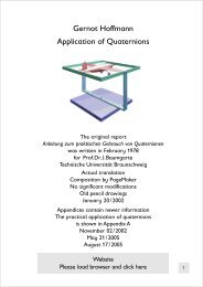
Gernot Hoffmann<br />
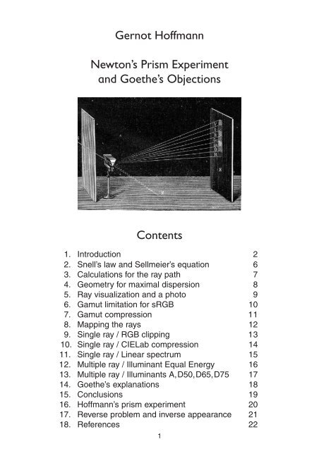
Newton’s <strong>Prism</strong> <strong>Experiment</strong><br />
<strong>and</strong> Goethe’s <strong>Objections</strong><br />
Contents<br />
1. Introduction 2<br />
2. Snell’s law <strong>and</strong> Sellmeier’s equation 6<br />
3. Calculations for the ray path 7<br />
4. Geometry for maximal dispersion 8<br />
5. Ray visualization <strong>and</strong> a photo 9<br />
6. Gamut limitation for sRGB 10<br />
7. Gamut compression 11<br />
8. Mapping the rays 12<br />
9. Single ray / RGB clipping 13<br />
10. Single ray / CIELab compression 14<br />
11. Single ray / Linear spectrum 15<br />
12. Multiple ray / Illuminant Equal Energy 16<br />
13. Multiple ray / Illuminants A,D50,D65,D75 17<br />
14. Goethe’s explanations 18<br />
15. Conclusions 19<br />
16. Hoffmann’s prism experiment 20<br />
17. Reverse problem <strong>and</strong> inverse appearance 21<br />
18. References 22<br />
1
1.1 Introduction / How to use this doc<br />
This document can be read by Adobe Acrobat. Some settings are essential: the color space<br />
sRGB for the appearance; the resolution 72dpi for pixel synchronized images.<br />
Best view zoom 200% (title image <strong>and</strong> photo on p.20).<br />
Settings for Acrobat<br />
Edit / Preferences / General / Page Display (since version 6)<br />
Custom Resolution 72dpi<br />
Edit / Preferences / General / Color Management (full version only)<br />
sRGB<br />
Euroscale Coated or ISO Coated or SWOP<br />
Gray Gamma 2.2<br />
A reasonable reproduction of the colors is possible only by a calibrated cathode ray tube<br />
monitor or a high end LCD monitor (no hope for notebooks or laptops).<br />
The monitor should be calibrated or adjusted by these test patterns:<br />
CalTutor<br />
http://www.fho-emden.de/~hoffmann/caltutor270900.pdf<br />
Printing this doc accurately requires a calibrated printer, preferably an inkjet or high end color<br />
laser printer. Office printers cannot reproduce the spectrum bars reasonably.<br />
Accurate printing requires a calibrated printer<br />
This document is protected by copyright. Any reproduction requires a permission by the author.<br />
This should be considered as a protection against bad or wrong copying. The author provides<br />
on dem<strong>and</strong> files in RGB for the specific purpose in original quality <strong>and</strong> files for CMYK offset<br />
printing (which cannot reproduce sRGB colors correctly), adjusted as good as possible.<br />
Copyright<br />
Gernot Hoffmann<br />
August 2005<br />
2
1.2 Introduction / About Newton<br />
Isaac Newton lived from 1642 to 1727. His work about optics <strong>and</strong> color was probably inspired<br />
by Descartes, Charleton, Boyle <strong>and</strong> Hook [5]. Refraction <strong>and</strong> dispersion by prisms were already<br />
known at this time, but Newton introduced 1666 a set of three crucial experiments (in fact by<br />
numerous experiments):<br />
1. Refraction <strong>and</strong> dispersion of a thin ray, which produces a spectrum b<strong>and</strong> with all rainbow<br />
colors: red, orange, yellow, green, blue, indigo <strong>and</strong> violet.<br />
2. Condensation of the spectrum b<strong>and</strong> by a lens. This delivers again white light.<br />
3. A spectral color, here a small part of the spectrum b<strong>and</strong>, can be refracted again but it<br />
cannot be further dispersed.<br />
Indigo was added - though not visible - in order to get a ‘harmonic’ sequence like the seven<br />
tones c,d,e,f,g,a,h,(c). The last tone c has double the frequency of the first. It is a strange<br />
coincidence that this ratio is approximately valid for the frequencies or wavelengths of visible<br />
light. In computer graphics we have a strong cyan between green <strong>and</strong> blue. In prism colors it<br />
is sometimes detectable - a better c<strong>and</strong>idate than indigo for the seventh rainbow color.<br />
Newton’s theories were by no means always clear <strong>and</strong> underst<strong>and</strong>able, which lead to lengthy<br />
<strong>and</strong> often rather impolite discussions between the most famous scientists in Europe.<br />
It is safe to say: Newton had discovered that white light consists of colored light.<br />
Newton arranged the spectrum on a circle. Drawing by<br />
the author, based on a print in Opticks [1].<br />
Connecting the ends of a spectrum like this does not<br />
have an equivalent for general electromagnetic or<br />
acoustical waves.<br />
This discovery was the first step towards spherical or<br />
cylindrical three-dimensional color spaces [7], [24].<br />
A segment of the circle is occupied by violet. Newton’s<br />
violet is complementary to yellow-green.<br />
In our present underst<strong>and</strong>ing this is mainly the magenta<br />
segment, but magenta is mixed by red <strong>and</strong> blue (violet)<br />
<strong>and</strong> not a spectral color.<br />
Newton says: ’That if the point Z fall in or near to the line OD, the main ingredients being the<br />
red <strong>and</strong> violet, the Colour compounded shall not be any of the prismatick Colours, but a<br />
purple, inclining to red or violet, accordingly as the point Z lieth on the side of the line DO<br />
towards E or towards C, <strong>and</strong> in general the compounded violet is more bright <strong>and</strong> more fiery<br />
than the uncompounded’.<br />
Newton knew already additive color mixing. He applied the center of gravity rule (which is<br />
accurately valid in the CIE chromaticity diagram) in his wheel. Z is such a mixture.<br />
The different refraction indices for different wavelengths lead Newton to the conclusion that<br />
telescopes with mirrors instead of lens’ should be more accurate. He manufactured such a<br />
telescope, using a metallic spherical mirror. The accuracy was probably affected by spherical<br />
aberration. At that time it was assumed that an ideal mirror should have the shape of a cone<br />
section but it was not yet discovered which one - a parabola. Manufacturing such a mirror<br />
would have been impossible.<br />
Newton published ’Opticks’ 1704, nearly forty years after his first experiments. In the time<br />
between he had spent much time developing mathematical methods, geometry <strong>and</strong> principles<br />
of mechanics.<br />
3<br />
D<br />
Red<br />
Violet<br />
E<br />
C<br />
Orange<br />
Z<br />
Indigo<br />
F<br />
O<br />
B<br />
Yellow<br />
Blew<br />
G<br />
A<br />
Green
1.3 Introduction / About Goethe<br />
Johann Wolfgang Goethe lived from 1749 to 1832. Well known as poet <strong>and</strong> writer, he was<br />
familiar as well with philosophy <strong>and</strong> natural science.<br />
1810 he published his book Geschichte der Farbenlehre [2]. This is mainly a historical review<br />
but as well a furious attack against Newton’s theories. Judging by our actual underst<strong>and</strong>ing of<br />
natural science, Goethe’s color theory was by no means well founded <strong>and</strong> elaborated. On the<br />
other h<strong>and</strong> he tried to integrate the aspects of culture <strong>and</strong> art in his generalizing concepts.<br />
The question remains: why did Goethe not believe in the Obvious in Newton’s theories ?<br />
It is the purpose of this document to demonstrate that the obvious in our present underst<strong>and</strong>ing<br />
was by no means obvious for Goethe. This demonstration will be done in an engineering<br />
style, based on many illustrations. These are accurate in the sense of classical optics <strong>and</strong> in<br />
the sense of actual color theory.<br />
The author found during his Google search nearly nowhere correct illustrations for the prism<br />
experiment. Drawings in publications are often wrong [5],[6], this could be a long list...<br />
One of the best illustrations is the title graphic, dated 1912 [8], but even here rules fantasy<br />
over reality: the blue-ish part is too small, indigo is in reality not perceivable <strong>and</strong> the geometrical<br />
path of the red ray is not accurate.<br />
4
1.4 Introduction / Goethe says...<br />
Some statements by Goethe, important in our context, may be quoted [2], followed by a<br />
simplified translation.<br />
A [2, Zweiter Teil, Konfession des Verfassers ]<br />
Aber wie verwundert war ich, als die durchs <strong>Prism</strong>a angeschaute weiße W<strong>and</strong> nach wie vor<br />
weiß blieb, daß nur da, wo ein Dunkles dran stieß, sich eine mehr oder weniger entschiedene<br />
Farbe zeigte, daß zuletzt die Fensterstäbe am allerlebhaftesten farbig erschienen, indessen<br />
am lichtgrauen Himmel draußen keine Spur von Färbung zu sehen war. Es bedurfte keiner<br />
langen Überlegung, so erkannte ich, daß eine Grenze notwendig sei, um Farben hervorzubringen,<br />
und ich sprach wie durch einen Instinkt sogleich vor mich laut aus, daß die Newtonische<br />
Lehre falsch sei.’<br />
’How surprised was I when I looked through a prism onto a white wall - still white, <strong>and</strong> colors<br />
appeared only there where dark met white. It was immediately clear that colors can appear<br />
only at boundaries. And I said loud, guided by an instinct: Newton’s teaching is wrong.’<br />
B [2, Zweiter Teil, Polemischer Teil ]<br />
’Also, um beim Refraktionsfalle zu verweilen, auf welchem sich die Newtonische Theorie<br />
doch eigentlich gründet, so ist es keineswegs die Brechung allein, welche die Farbenerscheinung<br />
verursacht; vielmehr bleibt eine zweite Bedingung unerläßlich, daß nämlich die<br />
Brechung auf ein Bild wirke und ein solches von der Stelle wegrücke.<br />
Ein Bild entsteht nur durch seine Grenzen; und diese Grenzen übersieht Newton ganz, ja er<br />
leugnet ihren Einfluß...und keines Bildes Mitte wird farbig, als insofern die farbigen Ränder<br />
sich berühren oder übergreifen.’<br />
’Again about the refraction, which is the true basis of Newton’s theory: color effects are not<br />
generated by refraction alone. A second necessary condition is, that refraction acts on an<br />
image by shifting it. An image is created merely by its boundaries, <strong>and</strong> these boundaries are<br />
not taken into account by Newton... <strong>and</strong> no image will become colorful in the middle, unless<br />
the colored boundaries touch or overlap each other.’<br />
C [2, Zweiter Teil, Beiträge zur Optik ]<br />
’Unter den eigentlichen farbigen Erscheinungen sind nur zwei, die uns einen ganz reinen<br />
Begriff geben, nämlich Gelb und Blau. Sie haben die besondere Eigenschaft, daß sie zusammen<br />
eine dritte Farbe hervorbringen, die wir Grün nennen.<br />
Dagegen kennen wir die rote Farbe nie in einem ganz reinen Zust<strong>and</strong>e: denn wir finden, daß<br />
sie sich entweder zum Gelben oder zum Blauen hinneigt.’<br />
’Only two colors can be considered as pure: yellow <strong>and</strong> blue. Their special feature is: they<br />
generate together a new color which we call green. Red is never pure: we find that this color<br />
tends either to yellow or to blue.’<br />
5
2. Snell’s law <strong>and</strong> Sellmeier’s equation<br />
The refraction of a ray which enters from a medium with refraction index n 1 into a medium with<br />
refraction index n 2 is defined by Snell’s law.<br />
The angles α <strong>and</strong> β are shown on the next page.The refraction index for air is practically 1.0.<br />
sin( b)<br />
n1<br />
1<br />
= =<br />
sin( a ) n2n Goethe said: Willebrord Snellius (1591-1626) knew the fundamentals but he did not know the<br />
definition by sine functions [2, Erster Teil, Fünfte Abteilung ].<br />
The refraction index as a function of the wavelength can be modelled by Sellmeier’s equation:<br />
2 B1<br />
n<br />
C<br />
2<br />
l<br />
( l)<br />
= 1+<br />
2<br />
l -<br />
1.80<br />
n<br />
1.75<br />
1.70<br />
1.65<br />
1.60<br />
1.55<br />
1<br />
2<br />
B2<br />
l<br />
+<br />
2<br />
l - C<br />
2<br />
SF15<br />
BK7<br />
1.50<br />
0.3 0.4 0.5 0.6 0.7 λ / µ m 0.8<br />
2<br />
B3<br />
l<br />
+<br />
2<br />
l - C<br />
3<br />
The structure of this function is essentially based on Maxwell’s theory of continua [4]. The<br />
function has three poles which are outside the spectrum of visible light. The poles indicate<br />
resonance phenomena without damping. In reality the peaks are finite because of damping.<br />
The actual parameters are found by measurements, here for special types of flint <strong>and</strong> crown<br />
glass.<br />
The refraction of flint glass is stronger. Because of the steeper slope the dispersion is stronger<br />
as well. Combinations of flint glass <strong>and</strong> crown glass can be used for achromatic lens or prism<br />
systems which show no dispersion for two distinct wavelengths <strong>and</strong> nearly no dispersions for<br />
the others. Goethe knew this already.<br />
Tables are supplied by Schott AG [15], here used for flint glass SF15. Thanks to Danny Rich.<br />
The Sellmeier equation <strong>and</strong> the data for crown glass BK7 were found at Wikipedia [16].<br />
6<br />
Glass SF15<br />
B1 1.539259<br />
B2 0.247621<br />
B3 1.038164<br />
C1 0.011931<br />
C2 0.055608<br />
C3 116.416755<br />
Glass BK7<br />
B1 1.039612<br />
B2 0.231792<br />
B3 1.010469<br />
C1 0.006001<br />
C2 0.020018<br />
C3 103.560653
3. Calculations for the ray path<br />
The path of the ray is calculated by intersections of line segments, using Snell’s law <strong>and</strong> some<br />
simple geometry: lines in parametric representation; solutions by Cramer’s rule. All direction<br />
vectors are normalized for unit length. The origin of u 1 is at C 1 .<br />
� 1<br />
R1 C1 u1 n1 d1 g1<br />
=<br />
È - sin( g)<br />
˘<br />
ÎÍ + cos( g)<br />
˚˙<br />
u1<br />
=<br />
È - sin( r1)<br />
˘<br />
ÎÍ - cos( r1)<br />
˚˙<br />
d1<br />
=<br />
È+<br />
cos( r 1)<br />
˘<br />
ÎÍ - sin( r1)<br />
˚˙<br />
r1 = c1+ uu1<br />
x1 = r1+ l d1<br />
x2 = m g1<br />
x1 = x2<br />
mg1 - ld1<br />
= r1<br />
m g1x - l d1x = r1x<br />
mg - ld<br />
= r<br />
1y 1y 1y<br />
� 1<br />
Solution by Cramer’s rule<br />
dA = d1xg1y - d g<br />
dM = d1 r1 -d1<br />
r1<br />
m = dM/ dA<br />
p1 = m g1<br />
a = g + r<br />
1 1<br />
1y 1x<br />
x y y x<br />
Refraction by Snell’s law<br />
sin( b ) = ( 1/<br />
n)sin(<br />
a )<br />
1 1<br />
P 1<br />
cos( b1) = 1-sin<br />
( b1)<br />
b1<br />
= a tan2<br />
[sin( b1),cos( b1)]<br />
d = g -b<br />
1 1<br />
2<br />
d 0<br />
� 1<br />
g 1<br />
�<br />
y<br />
g 2<br />
7<br />
� 2<br />
P 2<br />
d2 �2 � 2<br />
C 2<br />
u 2<br />
n 2<br />
g2<br />
=<br />
È + sin( g)<br />
˘<br />
ÎÍ + cos( g)<br />
˚˙<br />
d0<br />
=<br />
È+<br />
cos( d1)<br />
˘<br />
ÎÍ + sin(<br />
d1)<br />
˚˙<br />
x1 = p1+ l d0<br />
x2<br />
= m g2<br />
dA = d g -d<br />
g<br />
dM = d p -d<br />
p<br />
p2 = ( dM/ dA)<br />
g2<br />
b2= g + d<br />
sin( a ) = n sin( b )<br />
2 2<br />
n 1.5500<br />
rho1 45.0000<br />
rho2 45.0000<br />
alf1 75.0000<br />
bet1 38.5486<br />
alf2 34.5311<br />
bet2 21.4514<br />
defl 49.5311<br />
x<br />
R 2<br />
0x 2y 0y 2x<br />
0x 1y 0y 1x<br />
cos( a2) = 1-sin<br />
( a2)<br />
a = atan<br />
2 [ sin( a ),cos( a )]<br />
2 2 2<br />
u2<br />
=<br />
È + sin( r2)<br />
˘<br />
ÎÍ - cos( r2)<br />
˚˙<br />
d2 = a2 -g<br />
d2<br />
=<br />
È+<br />
cos( d2<br />
) ˘<br />
ÎÍ + sin( d2<br />
) ˚˙<br />
x1 = p2 + l d2<br />
x2 = c2 + mu2<br />
s2 = p2 -c2<br />
dA = d u -d<br />
u<br />
dM = d s -d<br />
s<br />
2<br />
2x 2y 2y 2x<br />
2x 2y 2y 2x<br />
r = c +( dM/ dA)<br />
u<br />
2 2 2
4. Geometry for maximal dispersion<br />
For a practical prism experiment the dispersion should be as large as possible. Flint glass is<br />
the better choice. The optimal angles can be found by trial <strong>and</strong> error.<br />
The simulation below confirms the test results. Left crown glass, right flint glass.The upper<br />
two images show the symmetrical case. The lower show the optimal case.The output angle β 2<br />
should be near to 90° for the shortest wavelength (violet).<br />
In the middle images one can see that large input angles α 1 do not deliver the best results.<br />
Glass BK7<br />
LBlue 0.3800<br />
LRed 0.7000<br />
nBlue 1.5337<br />
nRed 1.5131<br />
rho1 20.0000<br />
rho2 20.0000<br />
For blue<br />
alf1 50.0000<br />
bet1 29.9643<br />
alf2 50.1478<br />
bet2 30.0357<br />
defl 40.1478<br />
disp 1.8184<br />
Glass BK7<br />
LBlue 0.3800<br />
LRed 0.7000<br />
nBlue 1.5337<br />
nRed 1.5131<br />
rho1 52.0000<br />
rho2 0.0000<br />
For blue<br />
alf1 82.0000<br />
bet1 40.2147<br />
alf2 31.2764<br />
bet2 19.7853<br />
defl 53.2764<br />
disp 1.5672<br />
Glass BK7<br />
LBlue 0.3800<br />
LRed 0.7000<br />
nBlue 1.5337<br />
nRed 1.5131<br />
rho1 1.0000<br />
rho2 55.0000<br />
For blue<br />
alf1 31.0000<br />
bet1 19.6215<br />
alf2 83.5210<br />
bet2 40.3785<br />
defl 54.5210<br />
disp 6.4668<br />
Crown glass Flint glass<br />
8<br />
Glass SF15<br />
LBlue 0.3800<br />
LRed 0.7000<br />
nBlue 1.7548<br />
nRed 1.6890<br />
rho1 31.4000<br />
rho2 31.0000<br />
For blue<br />
alf1 61.4000<br />
bet1 30.0221<br />
alf2 61.2600<br />
bet2 29.9779<br />
defl 62.6600<br />
disp 7.1119<br />
Glass SF15<br />
LBlue 0.3800<br />
LRed 0.7000<br />
nBlue 1.7548<br />
nRed 1.6890<br />
rho1 55.0000<br />
rho2 19.0000<br />
For blue<br />
alf1 85.0000<br />
bet1 34.5899<br />
alf2 48.8484<br />
bet2 25.4101<br />
defl 73.8484<br />
disp 5.7646<br />
Glass SF15<br />
LBlue 0.3800<br />
LRed 0.7000<br />
nBlue 1.7548<br />
nRed 1.6890<br />
rho1 19.0000<br />
rho2 55.0000<br />
For blue<br />
alf1 49.0000<br />
bet1 25.4729<br />
alf2 84.0482<br />
bet2 34.5271<br />
defl 73.0482<br />
disp 15.4286
5. Ray visualization <strong>and</strong> a photo<br />
We are using throughout the document wavelengths from 0.380µm to 0.700µm. This range<br />
reaches from nearly invisible violet to nearly invisible red. The colors at the end of the spectrum<br />
can be made visible only by rather strong light sources in laboratories, 0.360µm to 0.800µm.<br />
A crude color visualization approximation is achieved by nonlinear HSB, a modification of the<br />
st<strong>and</strong>ard Hue-Saturation-Brightness model, which is represented by a cone [9], [24].<br />
This is a photo of a real spectrum bar. A little image processing was applied.<br />
9<br />
Glass SF15<br />
LBlue 0.3800<br />
LRed 0.7000<br />
nBlue 1.7548<br />
nRed 1.6890<br />
rho1 19.0000<br />
rho2 54.0000<br />
For blue<br />
alf1 49.0000<br />
bet1 25.4729<br />
alf2 84.0482<br />
bet2 34.5271<br />
defl 73.0482<br />
disp 15.4286
6. Gamut limitation for sRGB<br />
A correct visualization of the calculated spectrum bar would require media which can reproduce<br />
all spectral colors. This is not possible, not even by lasers. Especially one needs a plausible<br />
color reproduction on common cathode ray tube monitors (CRT monitors).<br />
The chromaticity diagram CIE xyY below is a special perspective projection of the physical<br />
color space CIE XYZ onto a plane. The area, filled symbolically by colors, represents the<br />
human gamut, but the luminance is left out. Spectral colors are on the horseshoe contour.<br />
The magenta line shows mixtures of violet <strong>and</strong> red. Magenta itself is not a spectral color.<br />
The magenta line is practically a fiction because the end points are nearly invisible in real life.<br />
Practical magentas are mixed by blue <strong>and</strong> red.<br />
Inside the horseshoe contour is the gamut triangle for sRGB (Rec.709 primaries <strong>and</strong> D65<br />
white point), but this triangle is the projection of an affine distorted cube. The gamut depends<br />
on the luminance as well, which is shown for increasing luminances Y=0.05 to 0.95 [22],[23].<br />
sRGB is a st<strong>and</strong>ardized color space, a reasonable model for real CRT monitors. Mapping<br />
spectral colors to sRGB is obviously very difficult. Especially vibrant oranges are missing.<br />
1.0<br />
y<br />
0.9<br />
0.8<br />
0.7<br />
0.6<br />
0.5<br />
0.4<br />
0.3<br />
0.2<br />
0.1<br />
520 525<br />
515 530<br />
535<br />
510<br />
540<br />
545<br />
550<br />
505<br />
555<br />
560<br />
565<br />
500<br />
570<br />
575<br />
580<br />
585<br />
495<br />
590<br />
595<br />
490<br />
0.95<br />
0.85<br />
0.75<br />
0.65<br />
0.55<br />
0.45<br />
600<br />
605<br />
610<br />
620<br />
635<br />
700<br />
485 0.35<br />
0.25<br />
480<br />
0.15<br />
475<br />
470<br />
0.05<br />
460<br />
380<br />
Magenta line<br />
0.0<br />
0.0 0.1 0.2 0.3 0.4 0.5 0.6 0.7 0.8 0.9 x 1.0<br />
10
7. Gamut compression<br />
7.1 Gamut compression Type A for single ray spectra in CIELab<br />
If the spectrum is generated by one ray, then the visualization by sRGB requires optimally<br />
saturated colors <strong>and</strong> a certain visual balance as well.<br />
If an orange cannot be shown brightly, then it is less convenient to show yellow in the neighbourhood<br />
as bright as possible.<br />
The blue part looks always too bright. This well-known phenomenon will be explained later.<br />
The gamut compression is done in CIELab [10],[21] by the author’s simple method. More<br />
subtle strategies for gamut compressions are described e.g. by Ján Morovic [14].<br />
Find the hue in Lab by a,b (asterisks L*.. omitted)<br />
Reduce the radius towards the L-axis until R,G,B<br />
are in-gamut<br />
This delivers a 1,b 1,L1 Modify L by<br />
L 2 = 0.5 + 0.7(L-0.5)<br />
Reduce the radius towards the L-axis until R,G,B<br />
are in-gamut<br />
This delivers a 2,b 2,L2 Apply a linear interpolation between 1 <strong>and</strong><br />
2 <strong>and</strong><br />
find the position with maximal saturation<br />
s = a 2 + b 2 /L<br />
7.2 Gamut compression Type B for multiple ray spectra in CIELab<br />
The complete compression as above is not useful for spectra which are generated by several<br />
rays. In this case the light in the middle is more or less white <strong>and</strong> an increased saturation<br />
would be wrong.<br />
The Lab luminance is simply multiplied by a factor of about 0.95 <strong>and</strong> only the first step of the<br />
compression is executed.<br />
7.3 Gamut compression Type C by RGB clipping<br />
Crude RGB clipping - even proportional clipping like here - does not deliver pleasant results.<br />
If R
8. Mapping the rays<br />
The upper image shows again the crude color approximation by nonlinear HSB, now with a<br />
smaller number of color rays.<br />
The lower image shows the content of an array with 1000+1 elements on the screen (right<br />
plane), starting approximately at the origin. Each color ray hits an element of this array.<br />
The wavelength is written into the array. Gaps are filled by linear interpolation.<br />
At position R we have many color rays per length, at position V fewer. In order to distribute the<br />
energy correctly across the length, the array content is multiplied by a slope factor. This is<br />
calculated by a linear interpolation of the slopes between sV <strong>and</strong> sR.<br />
The content of the array is converted into the color space CIE XYZ, using the common colormatching<br />
functions, <strong>and</strong> then converted to sRGB [10],[21],[22].<br />
Compression is here done by Type C, RGB clipping. The spectrum bar is shown b<strong>and</strong>ed.<br />
0.70<br />
0.66<br />
0.62<br />
0.58<br />
0.54<br />
0.50<br />
0.46<br />
0.42<br />
0.38<br />
λ / µ m<br />
sV<br />
0 1000<br />
12<br />
V<br />
R<br />
sR<br />
Glass SF15<br />
LBlue 0.3800<br />
LRed 0.7000<br />
nBlue 1.7548<br />
nRed 1.6890<br />
rho1 19.0000<br />
rho2 54.0000<br />
For blue<br />
alf1 49.0000<br />
bet1 25.4729<br />
alf2 84.0482<br />
bet2 34.5271<br />
defl 73.0482<br />
disp 15.4286
9. Single ray / Illuminant Equal Energy / Compr. Type C / RGB clipping<br />
Illuminant Equal Energy has a flat spectrum. Compression is done by Type C, RGB clipping.<br />
The spectrum bars are shown b<strong>and</strong>ed <strong>and</strong> continuous. The table shows linear RGB values,<br />
the bars were calculated with gamma encoding for sRGB. RGB clipping does not create<br />
balanced distributions of colors.<br />
No RGB clipping, no RGB gamma encoding<br />
Lam L* a* b* R G B<br />
0.38 0.0 5.5 -9.2 0.3 -0.3 1.8<br />
0.39 0.1 16.9 -25.0 0.9 -0.8 5.5<br />
0.40 0.4 53.0 -51.1 3.0 -2.6 18.5<br />
0.41 1.1 105.2 -85.6 9.1 -8.0 56.5<br />
0.42 3.6 175.9 -134.2 27.4 -24.5 175.7<br />
0.43 10.3 221.0 -171.4 53.9 -49.9 376.9<br />
0.44 17.0 215.6 -177.2 56.7 -56.6 474.6<br />
0.45 23.0 185.5 -168.0 37.6 -46.1 480.4<br />
0.46 29.4 141.2 -152.3 4.6 -25.5 450.9<br />
0.47 36.2 70.2 -121.5 -37.9 8.9 345.1<br />
0.48 44.1 -26.5 -77.8 -78.8 51.5 213.2<br />
0.49 52.7 -134.8 -32.1 -114.2 96.5 115.0<br />
0.50 63.6 -254.0 11.3 -157.2 156.2 56.6<br />
0.51 76.3 -290.7 53.9 -209.6 240.0 16.6<br />
0.52 87.5 -243.4 95.3 -236.0 324.8 -14.9 0.53 94.4 -196.6 122.7 -206.5 371.9 -31.1 0.54 98.2 -155.4 143.9 -136.6 384.8 -40.0 0.55 99.8 -114.3 159.6 -32.9 368.9 -43.2 0.56 99.8 -71.6 166.5 100.8 329.1 -42.3 0.57 98.1 -27.4 166.2 256.4 267.1 -38.1 0.58 94.7 16.6 161.0 416.0 189.7 -31.8 0.59 89.7 57.3 153.1 551.3 108.5 -24.5 0.60 83.5 90.0 142.8 630.4 39.3 -17.5 0.61 76.3 111.3 131.0 631.4 -7.2 -11.8 0.62 68.1 120.1 117.1 556.8 -28.9 -7.6<br />
0.63 58.5 117.6 100.8 427.0 -32.0 -4.7<br />
0.64 48.9 109.4 84.3 301.6 -27.0 -2.7<br />
0.65 39.1 96.7 67.4 192.4 -18.9 -1.5<br />
0.66 29.7 82.0 51.1 112.4 -11.6 -0.8<br />
0.67 20.8 66.9 35.9 59.7 -6.3 -0.4<br />
0.68 13.8 54.7 23.8 32.0 -3.4 -0.2<br />
0.69 7.4 43.1 12.8 15.5 -1.7 -0.1<br />
0.70 3.7 29.5 6.4 7.8 -0.9 -0.1<br />
0.70<br />
0.66<br />
0.62<br />
0.58<br />
0.54<br />
0.50<br />
0.46<br />
0.42<br />
0.38<br />
λ / µ m<br />
13<br />
With RGB clipping, no RGB gamma encoding<br />
Lam L* a* b* R G B<br />
0.38 0.7 4.2 -8.2 0.3 0.0 1.8<br />
0.39 2.1 12.9 -22.0 0.9 0.0 5.5<br />
0.40 7.0 34.1 -40.1 3.0 0.0 18.5<br />
0.41 17.3 49.7 -58.4 9.1 0.0 56.5<br />
0.42 32.4 72.4 -85.6 27.4 0.0 175.7<br />
0.43 40.8 83.1 -93.5 53.9 0.0 255.0<br />
0.44 41.1 83.3 -92.9 56.7 0.0 255.0<br />
0.45 38.5 81.8 -97.4 37.6 0.0 255.0<br />
0.46 33.1 79.5 -106.4 4.6 0.0 255.0<br />
0.47 37.3 64.0 -99.5 0.0 8.9 255.0<br />
0.48 52.4 13.7 -64.0 0.0 51.5 213.2<br />
0.49 61.9 -30.4 -17.2 0.0 96.5 115.0<br />
0.50 73.2 -60.1 26.0 0.0 156.2 56.6<br />
0.51 85.9 -81.4 67.1 0.0 240.0 16.6<br />
0.52 87.7 -86.2 83.2 0.0 255.0 0.0<br />
0.53 87.7 -86.2 83.2 0.0 255.0 0.0<br />
0.54 87.7 -86.2 83.2 0.0 255.0 0.0<br />
0.55 87.7 -86.2 83.2 0.0 255.0 0.0<br />
0.56 91.6 -54.9 87.9 100.8 255.0 0.0<br />
0.57 97.1 -21.6 94.5 255.0 255.0 0.0<br />
0.58 89.1 -6.4 88.7 255.0 189.7 0.0<br />
0.59 77.1 19.0 80.4 255.0 108.5 0.0<br />
0.60 63.6 51.7 72.0 255.0 39.3 0.0<br />
0.61 53.2 80.1 67.2 255.0 0.0 0.0<br />
0.62 53.2 80.1 67.2 255.0 0.0 0.0<br />
0.63 53.2 80.1 67.2 255.0 0.0 0.0<br />
0.64 53.2 80.1 67.2 255.0 0.0 0.0<br />
0.65 47.0 72.9 61.2 192.4 0.0 0.0<br />
0.66 36.7 60.9 51.1 112.4 0.0 0.0<br />
0.67 26.7 49.4 39.5 59.7 0.0 0.0<br />
0.68 18.7 40.1 28.7 32.0 0.0 0.0<br />
0.69 11.2 31.5 17.7 15.5 0.0 0.0<br />
0.70 5.9 24.1 9.3 7.8 0.0 0.0
10. Single ray / Illuminant Equal Energy / Compr. Type A / CIELab<br />
The same method as in the previous chapter, but now the compression is done by Type A in<br />
CIELab. The spectrum bars look better balanced.The table shows linear RGB values, the<br />
bars were calculated with gamma encoding for sRGB.The spectrum bars look better balanced<br />
because of CIELab gamut compression.<br />
No gamut compression, no RGB gamma encoding<br />
Lam L* a* b* R G B<br />
0.38 0.0 5.5 -9.2 0.3 -0.3 1.8<br />
0.39 0.1 16.9 -25.0 0.9 -0.8 5.5<br />
0.40 0.4 53.0 -51.1 3.0 -2.6 18.5<br />
0.41 1.1 105.2 -85.6 9.1 -8.0 56.5<br />
0.42 3.6 175.9 -134.2 27.4 -24.5 175.7<br />
0.43 10.3 221.0 -171.4 53.9 -49.9 376.9<br />
0.44 17.0 215.6 -177.2 56.7 -56.6 474.6<br />
0.45 23.0 185.5 -168.0 37.6 -46.1 480.4<br />
0.46 29.4 141.2 -152.3 4.6 -25.5 450.9<br />
0.47 36.2 70.2 -121.5 -37.9 8.9 345.1<br />
0.48 44.1 -26.5 -77.8 -78.8 51.5 213.2<br />
0.49 52.7 -134.8 -32.1 -114.2 96.5 115.0<br />
0.50 63.6 -254.0 11.3 -157.2 156.2 56.6<br />
0.51 76.3 -290.7 53.9 -209.6 240.0 16.6<br />
0.52 87.5 -243.4 95.3 -236.0 324.8 -14.9 0.53 94.4 -196.6 122.7 -206.5 371.9 -31.1 0.54 98.2 -155.4 143.9 -136.6 384.8 -40.0 0.55 99.8 -114.3 159.6 -32.9 368.9 -43.2 0.56 99.8 -71.6 166.5 100.8 329.1 -42.3 0.57 98.1 -27.4 166.2 256.4 267.1 -38.1 0.58 94.7 16.6 161.0 416.0 189.7 -31.8 0.59 89.7 57.3 153.1 551.3 108.5 -24.5 0.60 83.5 90.0 142.8 630.4 39.3 -17.5 0.61 76.3 111.3 131.0 631.4 -7.2 -11.8 0.62 68.1 120.1 117.1 556.8 -28.9 -7.6<br />
0.63 58.5 117.6 100.8 427.0 -32.0 -4.7<br />
0.64 48.9 109.4 84.3 301.6 -27.0 -2.7<br />
0.65 39.1 96.7 67.4 192.4 -18.9 -1.5<br />
0.66 29.7 82.0 51.1 112.4 -11.6 -0.8<br />
0.67 20.8 66.9 35.9 59.7 -6.3 -0.4<br />
0.68 13.8 54.7 23.8 32.0 -3.4 -0.2<br />
0.69 7.4 43.1 12.8 15.5 -1.7 -0.1<br />
0.70 3.7 29.5 6.4 7.8 -0.9 -0.1<br />
0.70<br />
0.66<br />
0.62<br />
0.58<br />
0.54<br />
0.50<br />
0.46<br />
0.42<br />
0.38<br />
λ / µ m<br />
14<br />
With gamut compression, no RGB gamma encoding<br />
Lam L* a* b* R G B<br />
0.38 0.0 0.2 -0.3 0.0 0.0 0.1<br />
0.39 0.1 0.7 -1.0 0.1 0.0 0.2<br />
0.40 0.4 2.0 -1.9 0.3 0.0 0.5<br />
0.41 1.1 5.8 -4.7 1.1 0.0 1.2<br />
0.42 3.6 18.9 -14.5 3.4 0.0 4.0<br />
0.43 10.3 34.9 -27.1 9.3 0.0 13.6<br />
0.44 17.0 44.4 -36.5 17.7 0.0 29.3<br />
0.45 23.0 53.6 -48.5 26.7 0.0 56.1<br />
0.46 29.4 65.6 -70.8 31.3 0.0 120.3<br />
0.47 36.2 49.8 -86.3 0.0 12.5 198.2<br />
0.48 44.1 -10.4 -30.7 0.1 41.1 83.3<br />
0.49 51.9 -31.5 -7.5 0.0 65.3 62.5<br />
0.50 59.5 -41.0 1.8 0.0 91.7 65.8<br />
0.51 68.4 -49.5 9.2 0.1 129.5 76.2<br />
0.52 76.2 -60.7 23.8 0.2 172.3 68.8<br />
0.53 81.1 -71.9 44.9 0.0 204.8 41.5<br />
0.54 83.7 -82.3 76.1 0.0 226.4 3.7<br />
0.55 84.9 -58.9 82.2 62.6 215.8 0.0<br />
0.56 84.9 -35.6 82.9 128.8 196.1 0.3<br />
0.57 83.7 -13.8 83.6 191.4 169.3 0.0<br />
0.58 81.3 8.5 82.8 250.6 136.0 0.3<br />
0.59 77.8 20.9 56.0 255.0 110.1 24.2<br />
0.60 73.4 31.0 49.2 254.5 85.1 26.4<br />
0.61 68.4 42.2 49.7 254.3 59.7 19.4<br />
0.62 62.7 55.6 54.3 254.9 34.4 10.2<br />
0.63 56.0 72.7 62.3 254.9 9.1 2.3<br />
0.64 49.2 75.8 58.4 213.4 0.0 1.5<br />
0.65 39.1 63.8 44.4 127.5 0.0 2.1<br />
0.66 29.7 53.4 33.3 72.9 0.0 2.0<br />
0.67 20.8 43.0 23.1 37.9 0.0 1.6<br />
0.68 13.8 34.7 15.1 19.9 0.0 1.2<br />
0.69 7.4 27.3 8.1 9.6 0.0 0.7<br />
0.70 3.7 17.2 3.7 4.8 0.0 0.4
11. Single Ray / Linear Spectrum / Illuminant Equal Energy /<br />
Compr. Type A / CIELab<br />
This is not the prism experiment. The wavelength is now linearly distributed along the horizontal<br />
axis. Graphics like this appear often in text books, mostly wrong though.<br />
Modern spectrophotometers use gratings instead of prisms.Then the bar would look like here.<br />
The table shows linear RGB values. Instead of Lab values (the same as on the previous page)<br />
the CIE XYZ values are shown. The bars were calculated with gamma encoding for sRGB.<br />
No gamut compression, no RGB gamma encoding<br />
Lam X 100 Y 100 Z 100 R G B<br />
0.38 0.1 0.0 0.6 0.3 -0.3 1.8<br />
0.39 0.4 0.0 2.0 0.9 -0.8 5.5<br />
0.40 1.4 0.0 6.8 3.0 -2.6 18.5<br />
0.41 4.4 0.1 20.7 9.1 -8.0 56.5<br />
0.42 13.4 0.4 64.6 27.4 -24.5 175.7<br />
0.43 28.4 1.2 138.6 53.9 -49.9 376.9<br />
0.44 34.8 2.3 174.7 56.7 -56.6 474.6<br />
0.45 33.6 3.8 177.2 37.6 -46.1 480.4<br />
0.46 29.1 6.0 166.9 4.6 -25.5 450.9<br />
0.47 19.5 9.1 128.8 -37.9 8.9 345.1<br />
0.48 9.6 13.9 81.3 -78.8 51.5 213.2<br />
0.49 3.2 20.8 46.5 -114.2 96.5 115.0<br />
0.50 0.5 32.3 27.2 -157.2 156.2 56.6<br />
0.51 0.9 50.3 15.8 -209.6 240.0 16.6<br />
0.52 6.3 71.0 7.8 -236.0 324.8 -14.9 0.53 16.5 86.2 4.2 -206.5 371.9 -31.1 0.54 29.0 95.4 2.0 -136.6 384.8 -40.0 0.55 43.3 99.5 0.9 -32.9 368.9 -43.2 0.56 59.4 99.5 0.4 100.8 329.1 -42.3 0.57 76.2 95.2 0.2 256.4 267.1 -38.1 0.58 91.6 87.0 0.2 416.0 189.7 -31.8 0.59 102.6 75.7 0.1 551.3 108.5 -24.5 0.60 106.2 63.1 0.1 630.4 39.3 -17.5 0.61 100.3 50.3 0.0 631.4 -7.2 -11.8 0.62 85.4 38.1 0.0 556.8 -28.9 -7.6<br />
0.63 64.2 26.5 0.0 427.0 -32.0 -4.7<br />
0.64 44.8 17.5 0.0 301.6 -27.0 -2.7<br />
0.65 28.3 10.7 0.0 192.4 -18.9 -1.5<br />
0.66 16.5 6.1 0.0 112.4 -11.6 -0.8<br />
0.67 8.7 3.2 -0.0 59.7 -6.3 -0.4<br />
0.68 4.7 1.7 0.0 32.0 -3.4 -0.2<br />
0.69 2.3 0.8 -0.0 15.5 -1.7 -0.1<br />
0.70 1.1 0.4 -0.0 7.8 -0.9 -0.1<br />
0.70<br />
0.66<br />
0.62<br />
0.58<br />
0.54<br />
0.50<br />
0.46<br />
0.42<br />
0.38<br />
λ / µ m<br />
15<br />
With gamut compression, no RGB gamma encoding<br />
Lam X 100 Y 100 Z 100 R G B<br />
0.38 0.0 0.0 0.0 0.0 0.0 0.1<br />
0.39 0.0 0.0 0.1 0.1 0.0 0.2<br />
0.40 0.1 0.0 0.2 0.3 0.0 0.5<br />
0.41 0.3 0.1 0.5 1.1 0.0 1.2<br />
0.42 0.8 0.4 1.5 3.4 0.0 4.0<br />
0.43 2.5 1.2 5.2 9.3 0.0 13.6<br />
0.44 4.9 2.3 11.1 17.7 0.0 29.3<br />
0.45 8.3 3.8 21.1 26.7 0.0 56.1<br />
0.46 13.6 6.0 45.1 31.3 0.0 120.3<br />
0.47 15.8 9.1 74.5 0.0 12.5 198.2<br />
0.48 11.7 13.9 33.0 0.1 41.1 83.3<br />
0.49 13.6 20.1 26.3 0.0 65.3 62.5<br />
0.50 17.5 27.6 28.8 0.0 91.7 65.8<br />
0.51 23.6 38.5 34.5 0.1 129.5 76.2<br />
0.52 29.1 50.3 33.7 0.2 172.3 68.8<br />
0.53 31.7 58.6 25.0 0.0 204.8 41.5<br />
0.54 32.0 63.6 12.0 0.0 226.4 3.7<br />
0.55 40.4 65.7 10.6 62.6 215.8 0.0<br />
0.56 48.3 65.7 10.3 128.8 196.1 0.3<br />
0.57 54.7 63.5 9.4 191.4 169.3 0.0<br />
0.58 59.6 59.0 8.4 250.6 136.0 0.3<br />
0.59 58.4 52.8 16.1 255.0 110.1 24.2<br />
0.60 55.0 45.8 15.7 254.5 85.1 26.4<br />
0.61 50.9 38.5 12.0 254.3 59.7 19.4<br />
0.62 46.8 31.2 7.3 254.9 34.4 10.2<br />
0.63 42.7 23.9 3.2 254.9 9.1 2.3<br />
0.64 34.6 17.8 2.2 213.4 0.0 1.5<br />
0.65 20.8 10.7 1.8 127.5 0.0 2.1<br />
0.66 11.9 6.1 1.3 72.9 0.0 2.0<br />
0.67 6.3 3.2 0.9 37.9 0.0 1.6<br />
0.68 3.3 1.7 0.6 19.9 0.0 1.2<br />
0.69 1.6 0.8 0.3 9.6 0.0 0.7<br />
0.70 0.8 0.4 0.2 4.8 0.0 0.4
12. Multiple ray / Illuminant Equal Energy / Compr. Type B / CIELab<br />
A continuous light b<strong>and</strong> with flat spectrum is simulated by multiple rays. Each of them is interpreted<br />
according to chapter 8. The content of the interpolated measurement array is multiplied<br />
by the color-matching functions <strong>and</strong> the slope function. Then summed up in a second array<br />
which contains CIE XYZ values for each wavelength. The content of the XYZ array is normalized<br />
for Ymax =1 after finishing the measurement. The sum approximates an integration.<br />
In the middle we have white light. At the ends we can see color fringes. This is Goethe’s<br />
important observation on which he based his attack against Newton: colors appear at the<br />
boundaries of light <strong>and</strong> shadow.<br />
0.70<br />
0.66<br />
0.62<br />
0.58<br />
0.54<br />
0.50<br />
0.46<br />
0.42<br />
0.38<br />
λ / µ m<br />
0 1000<br />
Illuminant Equal Energy<br />
16
13. Multiple ray / Illuminants A, D50, D65,D75 / Compr. Type B / CIELab<br />
Different illuminants generate different shades of white in the middle. Illuminant A is a Planckian<br />
radiator with color temperature 2856K, as produced by a domestic tungsten bulb. C<strong>and</strong>le<br />
light would look even ‘warmer’, which means it has a lower color temperature, about 1900K.<br />
Graphics for typical spectra are found in books [10] <strong>and</strong> in documents by the author [19].<br />
The values in the measurement array are multiplied by one of these spectra as well, in addition<br />
to the multiplication by color-matching functions <strong>and</strong> slope functions.<br />
In real life the discrepancies for different illuminants would be less obvious because of<br />
adaptation: the tungsten or c<strong>and</strong>le yellow would look less yellow-ish <strong>and</strong> north skylight D75<br />
would look less blue-ish.<br />
The simulation of perceived colors is h<strong>and</strong>led in color theory by chromatic adaptation transforms<br />
[10],[14],[21]. These are not applied here.<br />
0.70<br />
0.66<br />
0.62<br />
0.58<br />
0.54<br />
0.50<br />
0.46<br />
0.42<br />
0.38<br />
λ / µ m<br />
0 1000<br />
Illuminant A<br />
Illuminant D50<br />
Illuminant D65<br />
Illuminant D75<br />
17
14. Goethe’s explanations<br />
The graphic shows Goethe’s Fünfte Tafel. Here it is a new drawing by the author, based on a<br />
print in [2], as accurate as possible.<br />
The small image top left visualizes three situations for a light b<strong>and</strong>, represented by two rays:<br />
without refraction, refracted by a parallel plate <strong>and</strong> refracted by the upper prism. Color fringes<br />
are emphasized. The large image should make the refraction effect by one prism much clearer.<br />
The ray geometry in the prism (A) is wrong, but this is more a symbolical drawing which<br />
shows ’light versus shadow’.<br />
The cross-section (B) is approximately the same as in the previous chapters. But then said<br />
Goethe: ’the cross-section, where the ellipse is drawn, is about the one where Newton <strong>and</strong> his<br />
followers perceive, fix <strong>and</strong> measure the image’.<br />
Does it mean that Goethe expected a spectrum without white in the middle, like in the crosssections<br />
(C) to (E) ? Just an overlay of edge effects ? It seems so, but then he were terribly<br />
wrong - the rays in the middle cannot be ignored.<br />
Goethe used a light b<strong>and</strong>, Newton used for his crucial experiments a thin ray. And he knew<br />
already that light b<strong>and</strong>s deliver white in the middle.<br />
18<br />
A<br />
B<br />
C<br />
D<br />
E
15. Conclusions<br />
The Conclusions refer to the Introduction, chapter 1. Furtheron some remarks on the perceived<br />
brightness of blue are added.<br />
A [2, Zweiter Teil, Konfession des Verfassers ]<br />
Aber wie verwundert war ich, ...’<br />
A prism refracts a light b<strong>and</strong> or a dense bundle of (fictitious) rays without strong color effects<br />
in the middle because these rays sum up to white light. Goethe was not aware of this superposition.<br />
Therefore he emphasized color effects correctly at the boundary of the bundle.<br />
Newton’s crucial experiments were essentially done with thin rays.<br />
It is not underst<strong>and</strong>able why Goethe did not discuss the case for a thin ray. It seems that he<br />
regarded this as a quite unnatural test condition which had nothing to do with real life.<br />
In fact he did not read Opticks carefully or at all. For example, the ellipse (C) in his drawing<br />
was clearly described by Newton as ‘oblong’, the envelop of a sequence of circles.<br />
B [2, Zweiter Teil, Polemischer Teil ]<br />
’Also, um beim Refraktionsfalle zu verweilen, ...’<br />
Goethe assumes that refraction itself does not create color effects. This would require an<br />
image which is refracted <strong>and</strong> shifted as well, <strong>and</strong> which has boundaries, because it is an<br />
image. But if it is refracted then it is shifted - the argument is not underst<strong>and</strong>able.<br />
On the other h<strong>and</strong> he is right in a certain sense, though without being aware of: refraction<br />
itself does not colorize anything. The color or dispersion is a result of different refraction<br />
indices for different wavelengths, for different spectral colors.<br />
C [2, Zweiter Teil, Beiträge zur Optik ]<br />
’Unter den eigentlichen farbigen Erscheinungen sind nur zwei, ...’<br />
Goethe’s Erste Tafel shows color wheels. He had accepted Newton’s model to a certain extent.<br />
Goethe’s model uses (also according to [7]) three primaries yellow, blue, red <strong>and</strong> three<br />
secondaries orange, violet, green. On the other h<strong>and</strong> he considers only yellow <strong>and</strong> blue as<br />
pure colors. Maybe this was just an unnecessary complication.<br />
Goethe knew almost all the other contributors to color science, as mentioned in the same<br />
book [7], but not yet Philipp Otto Runge, who published 1810 the first threedimensional color<br />
space, a sphere.<br />
The Blue Mystery<br />
In simulations we perceive in the spectrum bars the small part for pure blue on monitors as<br />
too bright. The color reproduction is based on the sRGB model which describes with sufficient<br />
accuracy common cathode ray tube monitors (real monitors are calibrated by instruments, a<br />
process which introduces the actual parameters into the color management system).<br />
The contribution of blue to the luminance is given by equations like this:<br />
L = 0.3R + 0.6G + 0.1B<br />
With accurate numbers this is colorimetrically correct. Is blue really six or seven times darker<br />
than green ? The author could not prove such a ratio by flicker tests.<br />
An explanation might be the Helmholtz-Kohlrausch effect [13] which means: fully saturated<br />
colors appear brighter than less saturated colors. The table in chapter 10 shows the highest<br />
saturations for red at 0.63µm, for green at 0.54µm <strong>and</strong> for blue at 0.47µm.<br />
19
16. Hoffmann’s prism experiment<br />
A slide projector is used as light source. The slide is a metal plate with a thin horizontal slit.<br />
The cylinder with the prism can be rotated. The spectrum bar appears on an adjustable glass<br />
plate which is ground on one side. The mechanical system can be folded <strong>and</strong> stored together<br />
with the projector in a suitcase. A student’s project by Mr. Burhan Primanintyo.<br />
Best view zoom 200%.<br />
20
17. Reverse problem <strong>and</strong> inverse appearance<br />
In September 2012 the author received a message by Dr.Stephen R.J.Williams, a UK-based<br />
Geo-scientist:<br />
The images in your chapter 12 seem to explain how the fringes are produced. My interpretation<br />
(see attached illustration) of your diagram indicates that observer will see blue<br />
fringes at top of aperture image <strong>and</strong> red/yellow fringes at bottom of aperture image.<br />
But when I look through a real prism I see blue fringes at the bottom of the aperture<br />
image <strong>and</strong> red/yellow fringes at the top. This is opposite to that in the diagram.<br />
Dr.Williams is right. Later he provided the link [26], which is of high value. But this report does<br />
not explain the problem in a convincing manner, does not explain what is called below the<br />
inverse appearance phenomenon.<br />
Not even Goethe himself had described the discrepancy between his drawing Fünfte Tafel in<br />
chapter 14 <strong>and</strong> his view through the prism. The drawing reproduces more or less Newton‘s<br />
approach (with some errors though, concerning the angles of refraction). It shows the color<br />
b<strong>and</strong>s on a screen, similar to all the other illustrations here in this document.<br />
Looking through a prism is in [26] called the reverse problem - exactly Goethe‘s approach, but<br />
not in his drawing. The inversion, as observed by Dr.Williams, is here called inverse appearance<br />
phenomenon.<br />
The explanation follows Dr.Williams‘ idea with minor modifications. At the left we have a black<br />
card board with a white rectangle, maybe like one of those which Goethe had used [27].<br />
One eye of the observer is shown at the right. We are interpreting two rays R 1 <strong>and</strong> R 2 . Ray R 1<br />
could be generated by a violet ray v 1 , a red ray r 1 or any other ray between (in modern nomenclature:<br />
orange, yellow, green, cyan, blue). Now we see that blue, cyan <strong>and</strong> green actually<br />
cannot be generated, because the card board is black at these positions. Therefore only red<br />
<strong>and</strong> yellow contributions remain <strong>and</strong> that is the color of the fringe. For ray R 2 the situation is<br />
similar, but violet, blue <strong>and</strong> cyan remain. Dr.Williams emphasizes that green hardly appears at<br />
edges, opposed to fully developed rainbow spectra for narrow apertures or rectangles. This<br />
can be confirmed by experiments using the Goethe Kit [27].<br />
Somewhat simplified: the top fringe is red/yellow, the bottom fringe blue/cyan. This is indeed<br />
an inverse appearance, compared to the projection of rays through a prism onto a screen, as<br />
simulated in chapter 12.<br />
r 2<br />
v1 r1 v2 21<br />
R 1<br />
R 2<br />
Eye
18.1 References<br />
[1] Isaac Newton<br />
Opticks<br />
Great Mind Series, Prometheus, 2003<br />
[2] Johann Wolfgang Goethe<br />
Geschichte der Farbenlehre<br />
Erster Teil, zweiter Teil, dtv Gesamtausgabe 41,42<br />
Deutscher Taschenbuchverlag, München, 1963<br />
Thanks to Volker Hoffmann for preserving <strong>and</strong> providing the book<br />
[3] W.Heisenberg<br />
Die Goethe’sche und die Newton’sche Farbenlehre im Lichte der modernen Physik<br />
W<strong>and</strong>lungen in den Grundlagen der Naturwissenschaft. 4.Auflage, Verlag S.Hirzel, Leipzig, 1943<br />
[4] Chr.Gerthsen<br />
Physik<br />
Springer Verlag, Berlin..., 1966<br />
[5] N.Guicciardini<br />
Newton: Ein Naturphilosoph und das System der Welten<br />
Spektrum der Wisssenschaft Verlagsgesellschaft, Heidelberg, 1999<br />
[6] R.Breuer (Chefredakteur)<br />
Farben<br />
Spektrum der Wisssenschaft Verlagsgesellschaft, Heidelberg, 2000<br />
[7] N.Silvestrini + E.P.Fischer<br />
Idee Farbe, Farbsysteme in Kunst und Wissenschaft<br />
Baumann & Stromer Verlag, Zürich, 1994<br />
[8] K.Kahnmeyer + H.Schulze<br />
Realienbuch<br />
Velhagen & Klasing, Bielefeld und Leipzig, 1912<br />
[9] J.D.Foley + A.van Dam + St.K.Feiner + J.F.Hughes<br />
Computer Graphics<br />
Addison-Wesley, Reading Massachusetts,...,1993<br />
[10] R.W.G.Hunt<br />
Measuring Colour<br />
Fountain Press, Engl<strong>and</strong>, 1998<br />
[11] R.W.G.Hunt<br />
The Reproduction of Colour, sixth edition<br />
John Wiley & Sons, Chichester, Engl<strong>and</strong>, 2004<br />
[12] E.J.Giorgianni + Th.E.Madden<br />
Digital Color Management<br />
Addison-Wesley, Reading Massachusetts ,..., 1998<br />
[13] G.Wyszecki + W.S. Stiles<br />
Color Science<br />
John Wiley & Sons, New York ,..., 1982<br />
[14] Ph.Green + L.MacDonald (Ed.)<br />
Colour Engineering<br />
John Wiley & Sons, Chichester, Engl<strong>and</strong>, 2002<br />
22
18.2 References<br />
[15] Schott AG<br />
Optischer Glaskatalog - Datentabelle EXCEL 28.04.2005<br />
http://www.schott.com<br />
[16] Wikipedia<br />
Sellmeier Equation<br />
http://en.wikipedia.org/wiki/Sellmeier_equation<br />
[17] M.Stokes + M.Anderson + S.Ch<strong>and</strong>rasekar + R.Motta<br />
A St<strong>and</strong>ard Default Color Space for the Internet - sRGB, 1996<br />
http://www.w3.org/graphics/color/srgb.html<br />
[19] G.Hoffmann<br />
Documents, mainly about computer vision<br />
http://www.fho-emden.de/~hoffmann/howww41a.html<br />
[20] G.Hoffmann<br />
Hardware Monitor Calibration<br />
http://www.fho-emden.de/~hoffmann/caltutor270900.pdf<br />
[21] G.Hoffmann<br />
CIELab Color Space<br />
http://www.fho-emden.de/~hoffmann/cielab03022003.pdf<br />
[22] G.Hoffmann<br />
CIE (1931) Color Space<br />
http://www.fho-emden.de/~hoffmann/ciexyz29082000.pdf<br />
[23] G.Hoffmann<br />
Gamut for CIE Primaries with Varying Luminance<br />
http://www.fho-emden.de/~hoffmann/ciegamut16012003.pdf<br />
[24] G.Hoffmann<br />
Color Order Systems RGB / HLS / HSB<br />
http://www.fho-emden.de/~hoffmann/hlscone03052001.pdf<br />
[25] Earl F.Glynn<br />
Collection of links, everything about color <strong>and</strong> computers<br />
http://www.efg2.com<br />
[26] Zur Farbenlehre (in English, author unknown)<br />
http://www.mathpages.com/home/kmath608/kmath608.htm<br />
[27] Goethes <strong>Experiment</strong>e zu Licht und Farbe<br />
<strong>Experiment</strong>al kit with prism, Goethe‘s color cards, posters, textbook <strong>and</strong> facsimile print<br />
of Goethe‘s Beyträge zur Optik (1791)<br />
Klassik Stiftung Weimar 2007<br />
Verlag Bien & Giersch Projektagentur<br />
This doc<br />
http://www.fho-emden.de/~hoffmann/prism16072005.pdf<br />
Gernot Hoffmann<br />
September 15 / 2005 + October 16 / 2012<br />
Website<br />
Load browser / Click here<br />
23


![[PDF] SpieleProgrammierung](https://img.yumpu.com/6860251/1/190x135/pdf-spieleprogrammierung.jpg?quality=85)