Drift 2

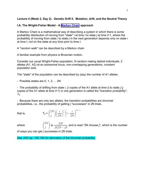
1Lecture 4 (Week 2, Day 2). Genetic Drift II. Mutation, drift, and the Neutral TheoryI.A. The Wright-Fisher Model - A Markov Chain approachA Markov Chain is a mathematical way of describing a system in which there is someprobability distribution of moving from "state" i at time t to state j at time t+1, where theprobability of moving from state i to state j in the next generation depends only on state iat time t, not on the state at any time prior to time t.A "random walk" can be described by a Markov chainA familiar example from physics is Brownian motion.Consider our usual Wright-Fisher population, N random mating diploid individuals, 2alleles (A1, A2) at an autosomal locus, non-overlapping generations, constantpopulation size.The "state" of the population can be described by (say) the number of A1 alleles.- Possible states are 0, 1, 2, ... 2N- The probability of drifting from state i, (i copies of the A1 allele at time t) to state j (jcopies of the A1 allele at time t+1) in one generation is called the "transition probability",T ij .- Because there are only two alleles, the transition probabilities are binomialprobabilities, i.e., the probability of getting j "successes" in 2N trials.⎛2N⎞ ⎛that is, T ij = ⎜ ⎟ ⎜⎝ j ⎠ ⎝ 2iNj⎞⎟⎠2⎛ i ⎞⎜1− ⎟⎝ 2N⎠N − j⎛2N⎞ 2N!where⎜ ⎟ isand is read "2N choose j", which is the number⎝ j ⎠ j!(2N− j)!of ways you can get j successes in 2N trials.See JHG pp. 192-194 for derivation of the binomial probability.

3I.B The Stationary DistributionA different way of thinking of genetic drift rather than the probability of a singlepopulation having a particular state is as the probability distribution of a large number ofreplicate populations with similar properties.Let X i be a random variable that denotes the frequency of populations having i copies ofthe A1 allele (i.e., being in state i, i = 0, 1, 2, ... 2N)Let X be the ROW vector of X i , i.e., [X 0 , X 1 , X 2 , ... X N ]After one generation of genetic drift, X' = XT2NX ii=0where Xj ' = ∑T ij-------------------------------------------------------------------------------------------------------NOTES on matrix multiplication (from H. Anton, "Elementary Linear Algebra")Definition: If A is an m x r matrix and B is an r x n matrix, then the PRODUCT ABis the m x n matrix whose entries are determined as follows. To find the entry inrow i and column j of AB, single out row i from the matrix A and the column j fromthe matrix B. Multiply the corresponding entries from the row and columntogether and then add up the resulting products.For example:A = 1 2 4 and B = 4 1 4 32 6 0 0 -1 3 12 7 5 2Since A is a 2x3 matrix and B is a 3x4 matrix, the product AB is a 2x4 matrix. Todetermine, say, the entry in row 2, column 3 of AB, single out row 2 from A and column3 from B. Then, multiply corresponding entries together and add up these products.1 2 4 4 1 4 3 x x x x2 6 0 0 -1 3 1 = x x 26 x2 7 5 2For more in-depth information on matrix multiplication, check out the following websites.http://mathworld.wolfram.com/MatrixMultiplication.htmlhttp://www.mai.liu.se/~halun/matrix/matrix.html

5The mean of a binomial random variable with parameters n (= 2N) and p = 2Np, Var =2NpqLet p' = X/2N, so E[p'] = E[X]/2N = 2Np/2N = pVar(p') = Var[X]/4N 2 = pq/2NSee JHG Equation B.12 for derivationDefine N e as the size of an ideal Wright-Fisher population with Var(p') = pq/2N, calledthe "variance effective size"In words, N e is the size of an ideal W-F population that undergoes an equivalent amountof genetic drift as the real population in question.- Two special cases of N e1. Fluctuating population size (N not constant)1/N e = (1/N 1 + 1/N 2 +...1/N t )N e = the "harmonic" meane.g., N 1 = 1000, N 2 = 10, N 3 = 1000, N e = 29.4, (arithmetic mean N = 670)2. Unequal sex ratio (i.e., in a dioecious species)N e = 4N m N f /(N f + N m )e.g., N m =10, N f = 100, Ne = 36.4III. Mutation and DriftDrift removes variation, mutation puts it back in. Now we'll see what happens when weviolate the second H-W assumption, i.e., no mutation.III.A. Rate of change of allele frequency under mutation alone- Let A1 → A2 = u- Let A2 → A1 = vSo, p' = p(1-u) + (1-p)vIn words, the frequency of the A1 allele in the next generation is the frequency in thecurrent generation (p) multiplied by the probability an A1 allele does not mutate (1-u)

6PLUS the frequency of A2 alleles (q) multiplied by the probability that an A2 mutates toan A1, which is v.We can write a recursion in terms of p 0 : p t = (v/u+v) + [p 0 - (v/u+v)](1-u-v) tTwo important points emerge from this recursion:1. When t is small, (1-u-v) t ≈ 1-t(u+v). If p 0 = 0, then p t ≈ tvSo, p increases linearly with time, but the rate is very slow because v is small2. As t→ ∞, (1-u-v) t → 0, so p^ = v/(u+v)III.B. Mutation and Drift- Mutation introduces new alleles into the population at rate 2Nu- Drift removes variation at rate 1/2N (JHG equation 2.1)Recall G, the probability that two alleles that are different by origin are identical by state.After one generation of random mating and mutation,G ' = (1-u) 2 [(1/2N) + (1-1/2N)G]To see why this is, note that Pr(1st allele didn't mutate) = 1-u, so Pr(neither allelemutated) = (1-u)(1-u) = (1-u) 2 .Now we can use three approximations of the sort that theoreticians love to use to baffleempiricists.1) (1-u) 2 ≈ 1-2u if u is small [because (1-u)(1-u) = 1-2u+u 2 and u 2 is really small]2) Ignore terms with u/N, because u is small and N is large, so u/N is really small3) Let H = 1-G and rearrange to get H ' ≈ (1-1/2N)H + 2u(1-H)So, ΔH = -(1/2N)H + 2u(1-H) JHG Equation 2.9At equilibrium ΔH = 0, so H^ = 4Nu/(1+4Nu)and G^ = 1/(1+4Nu)- We can express Equ'n 2.9 as: Δ N H + Δ u HNote that for a given H, Δ N H depends only on N and Δ u H depends only on u

7- In an infinite population, 1/2N → 0, so H ' = H + (1-H)[1-(1-u) 2 ], so approximating(1-u) 2 as 1+2u, we get: H ' = Δ u H JHG Equation 2.11This result has three important implications:1. Δ u H ≥ 0. Mutation always increases genetic variation2. If 4Nu > 1, H^ → 1.So, the amount of genetic variation in a population at equilibrium depends on the size ofthe population as well as the mutation rate.IV. The Neutral Theory, Part I.What follows is a very brief and heuristic derivation of perhaps the most important resultin population genetics.There are 2N alleles ("copies of the gene") in the population.The probability that one mutates is u (the mutation rate)So, the number of mutations entering a population in a generation is 2Nu.The probability that a new, neutral mutation reaches fixation is just it's frequency in thepopulation, which is 1/2N.So, (# new mutations / gen)(Probability that a new mutation fixes) = (2Nu)(1/2N) = u.Note that here "u" is expressed in number of fixations per generation.The rate of fixation, (the "substitution rate") which we will call k, is the mutation rate, u.k = uFor example, suppose the mutation rate u is 1/100, and the population size N=50, so2N=100. Thus, every generation, on average, one new mutation occurs(2Nu=100*1/100=1). The probability that that new mutation ultimately reaches fixationis 1/2N, i.e., 1/100. So on average, every 100 generations a new fixation occurs, i.e.,one allele is substituted for another. Thus, the probability that a new fixation occurs inany particular generation is 1/100, which is the mutation rate.