RTDAQ software - Campbell Scientific

Campbell Scientific, Inc.Software End User License Agreement(EULA)NOTICE OF AGREEMENT: This software is copyrighted software. Pleasecarefully read this EULA. By installing or using this software, you are agreeingto comply with the following terms and conditions. If you do not want to bebound by this EULA, you must promptly return the software, any copies, andaccompanying documentation in its original packaging to Campbell Scientificor its representative.This software can be installed as a trial version or as a fully licensed copy. Allterms and conditions contained herein apply to both versions of software unlessexplicitly stated.TRIAL VERSION: Campbell Scientific distributes a trial version of thissoftware free of charge to enable users to work with Campbell Scientific dataacquisition equipment. You may use the trial version of this software for 30days on a single computer. After that period has ended, to continue using thisproduct you must purchase a fully licensed version.This trial may be freely copied. However, you are prohibited from charging inany way for any such copies and from distributing the software and/or thedocumentation with any other products (commercial or otherwise) withoutprior written permission from Campbell Scientific.LICENSE FOR USE: Campbell Scientific grants you a non-exclusive licenseto use this software in accordance with the following:(1) The purchase of this software allows you to install and use the software onone computer only.(2) This software cannot be loaded on a network server for the purposes ofdistribution or for access to the software by multiple operators. If thesoftware can be used from any computer other than the computer on whichit is installed, you must license a copy of the software for each additionalcomputer from which the software may be accessed.(3) If this copy of the software is an upgrade from a previous version, youmust possess a valid license for the earlier version of software. You maycontinue to use the earlier copy of software only if the upgrade copy andearlier version are installed and used on the same computer. The earlierversion of software may not be installed and used on a separate computeror transferred to another party.(4) This software package is licensed as a single product. Its component partsmay not be separated for use on more than one computer.(5) You may make one (1) backup copy of this software onto media similar tothe original distribution, to protect your investment in the software in caseof damage or loss. This backup copy can be used only to replace anunusable copy of the original installation media.

WARRANTIES: The following warranties are in effect for ninety (90) daysfrom the date of shipment of the original purchase. These warranties are notextended by the installation of upgrades or patches offered free of charge.Campbell Scientific warrants that the installation media on which the softwareis recorded and the documentation provided with it are free from physicaldefects in materials and workmanship under normal use. The warranty does notcover any installation media that has been damaged, lost, or abused. You areurged to make a backup copy (as set forth above) to protect your investment.Damaged or lost media is the sole responsibility of the licensee and will not bereplaced by Campbell Scientific.Campbell Scientific warrants that the software itself will perform substantiallyin accordance with the specifications set forth in the instruction manual whenproperly installed and used in a manner consistent with the publishedrecommendations, including recommended system requirements. CampbellScientific does not warrant that the software will meet licensee’s requirementsfor use, or that the software or documentation are error free, or that theoperation of the software will be uninterrupted.Campbell Scientific will either replace or correct any software that does notperform substantially according to the specifications set forth in the instructionmanual with a corrected copy of the software or corrective code. In the case ofsignificant error in the installation media or documentation, CampbellScientific will correct errors without charge by providing new media, addenda,or substitute pages. If Campbell Scientific is unable to replace defective mediaor documentation, or if it is unable to provide corrected software or correcteddocumentation within a reasonable time, it will either replace the software witha functionally similar program or refund the purchase price paid for thesoftware.All warranties of merchantability and fitness for a particular purpose aredisclaimed and excluded. Campbell Scientific shall not in any case be liable forspecial, incidental, consequential, indirect, or other similar damages even ifCampbell Scientific has been advised of the possibility of such damages.Campbell Scientific is not responsible for any costs incurred as a result of lostprofits or revenue, loss of use of the software, loss of data, cost of re-creatinglost data, the cost of any substitute program, telecommunication access costs,claims by any party other than licensee, or for other similar costs.This warranty does not cover any software that has been altered or changed inany way by anyone other than Campbell Scientific. Campbell Scientific is notresponsible for problems caused by computer hardware, computer operatingsystems, or the use of Campbell Scientific’s software with non-CampbellScientific software.Licensee’s sole and exclusive remedy is set forth in this limited warranty.Campbell Scientific’s aggregate liability arising from or relating to thisagreement or the software or documentation (regardless of the form of action;e.g., contract, tort, computer malpractice, fraud and/or otherwise) is limited tothe purchase price paid by the licensee.COPYRIGHT: This software is protected by United States copyright law andinternational copyright treaty provisions. This software may not be sold,included or redistributed in any other software, or altered in any way withoutprior written permission from Campbell Scientific. All copyright notices andlabeling must be left intact.

RTDAQ Table of ContentsPDF viewers: These page numbers refer to the printed version of this document. Use thePDF reader bookmarks tab for links to specific sections.Preface — What's New in RTDAQ? ................................ xi1. Introduction...............................................................1-11.1 RTDAQ Overview................................................................................ 1-21.1.1 Main Screen ................................................................................ 1-21.1.2 Clock/Program and the EZSetup Wizard.................................... 1-31.1.3 Monitor Data............................................................................... 1-31.1.3.1 Real-time Monitors............................................................ 1-31.1.4 Collect Data ................................................................................ 1-61.1.5 Field Calibration and the Calibration Wizard ............................. 1-71.1.6 RTMC Development, Run-time and Pro Development .............. 1-71.1.7 View Pro ..................................................................................... 1-81.1.8 Split............................................................................................. 1-91.1.9 CardConvert................................................................................ 1-91.1.10 Short Cut................................................................................... 1-91.1.11 CRBasic Editor ....................................................................... 1-101.1.12 CR5000/CR9000X Program Generators................................. 1-101.2 Getting Help for RTDAQ Applications.............................................. 1-111.3 Windows Conventions........................................................................ 1-112. System Requirements ..............................................2-12.1 Hardware and Software ........................................................................ 2-13. Installation, Operation and Backup Procedures....3-13.1 CD-ROM Installation ........................................................................... 3-13.2 RTDAQ Operations and Backup Procedures ....................................... 3-23.2.1 RTDAQ Directory Structure and File Descriptions.................... 3-23.2.1.1 Program Directory............................................................. 3-23.2.1.2 Working Directories.......................................................... 3-23.2.2 Backing up the Network Map and Data Files ............................. 3-33.2.2.1 Performing a Backup......................................................... 3-43.2.2.2 Restoring the Network from a Backup File....................... 3-43.2.3 Loss of Computer Power ............................................................ 3-44. The RTDAQ Main Screen .........................................4-14.1 Overview .............................................................................................. 4-14.1.1 Program Startup and Main Screen Functionality........................ 4-14.1.2 Datalogger Connectivity, Help and Program Exit ...................... 4-34.2 EZSetup Wizard ................................................................................... 4-34.2.1 Add Datalogger........................................................................... 4-34.2.2 Communication Setup................................................................. 4-4i

RTDAQ Table of Contents4.2.3 Datalogger Settings ..................................................................... 4-44.2.3.1 Max Time Online............................................................... 4-54.2.4 Summary, Communications Test, and Clock Set........................ 4-54.2.5 Send Program.............................................................................. 4-54.2.6 Editing and Deleting Dataloggers ............................................... 4-54.3 Clock/Program Tab............................................................................... 4-64.3.1 Basic Operation........................................................................... 4-64.4 Monitor Data Tab.................................................................................. 4-74.4.1 Field Monitor .............................................................................. 4-74.4.2 Editing Variable Values .............................................................. 4-74.4.3 Specialized Real-time Monitor Screens ...................................... 4-84.5 Collect Data Tab ................................................................................... 4-84.6 Pull-down Menus.................................................................................. 4-94.6.1 File Menu .................................................................................... 4-94.6.1.1 Saving and Loading Configurations.................................. 4-94.6.1.2 Exit .................................................................................... 4-94.6.2 View Menu.................................................................................. 4-94.6.3 Datalogger Menu....................................................................... 4-104.6.3.1 Connect/Disconnect......................................................... 4-104.6.3.2 Update Table Definitions................................................. 4-104.6.3.3 Status Table ..................................................................... 4-104.6.3.4 File Control...................................................................... 4-124.6.3.5 Calibration Wizard .......................................................... 4-154.6.3.6 Terminal Emulator........................................................... 4-164.6.4 Network Menu .......................................................................... 4-174.6.4.1 Add/Delete/Edit/Rename Datalogger .............................. 4-174.6.4.2 Backup/Restore Network................................................. 4-174.6.4.3 Computer’s Global PakBus Address ............................... 4-174.6.5 Tools Menu ............................................................................... 4-184.6.5.1 Auxiliary Applications .................................................... 4-184.6.5.2 Options ............................................................................ 4-194.6.5.3 LogTool ........................................................................... 4-194.6.5.4 PakBus Graph.................................................................. 4-214.7 The RTDAQ Toolbar.......................................................................... 4-235. Program Creation and Editing ................................ 5-15.1 CRBasic Editor ..................................................................................... 5-15.1.1 Overview..................................................................................... 5-15.1.2 Inserting Instructions................................................................... 5-25.1.2.1 Parameter Dialog Box ....................................................... 5-25.1.2.2 Right-Click Functionality .................................................. 5-45.1.3 Toolbar ........................................................................................ 5-55.1.3.1 Compile ............................................................................. 5-75.1.3.2 Compile, Save, and Send................................................... 5-85.1.3.3 Conditional Compile and Save ........................................ 5-115.1.3.4 Templates......................................................................... 5-115.1.3.5 Program Navigation using BookMarks and GoTo .......... 5-125.1.3.6 CRBasic Editor File Menu............................................... 5-125.1.3.7 CRBasic Editor Edit Menu .............................................. 5-135.1.3.8 CRBasic Editor View Menu ............................................ 5-135.1.3.9 CRBasic Editor Tools Menu............................................ 5-165.1.3.10 Available Help Information........................................... 5-19ii

RTDAQ Table of Contents5.1.4 CRBasic Programming ............................................................. 5-205.1.4.1 Programming Sequence................................................... 5-205.1.4.2 Program Declarations...................................................... 5-215.1.4.3 Mathematical Expressions............................................... 5-215.1.4.4 Measurement and Output Processing Instructions .......... 5-225.1.4.5 Line Continuation............................................................ 5-225.1.4.6 Inserting Comments Into Program .................................. 5-235.1.4.7 Example Program............................................................ 5-245.1.4.8 Data Tables...................................................................... 5-245.1.4.9 The Scan -- Measurement Timing and Processing.......... 5-265.1.4.10 Numerical Entries.......................................................... 5-275.1.4.11 Logical Expression Evaluation...................................... 5-275.1.4.12 Flags .............................................................................. 5-295.1.4.13 Parameter Types............................................................ 5-295.1.4.14 Program Access to Data Tables..................................... 5-305.2 Short Cut............................................................................................. 5-315.2.1 Overview................................................................................... 5-315.2.2 Creating a Program Using Short Cut ........................................ 5-325.2.2.1 Step 1 – Create a New File or Open Existing File .......... 5-335.2.2.2 Step 2 – Select Datalogger and Specify Scan Interval .... 5-335.2.2.3 Step 3 – Choose Sensors to Monitor ............................... 5-365.2.2.4 Step 4 – Setup Output Tables.......................................... 5-435.2.2.5 Step 5 – Generate the Program in the Format Requiredby the Datalogger .................................................................. 5-465.2.3 Short Cut Settings ..................................................................... 5-475.2.3.1 Program Security............................................................. 5-475.2.3.2 Datalogger ID.................................................................. 5-475.2.3.3 Power-up Settings ........................................................... 5-475.2.3.4 Select CR200 Compiler................................................... 5-485.2.3.5 Sensor Support ................................................................ 5-485.2.3.6 Integration ....................................................................... 5-495.2.3.7 Font ................................................................................. 5-495.2.3.8 Set Working Directory .................................................... 5-495.2.3.9 Enable Creation of Custom Sensor Files......................... 5-495.2.4 Editing Programs Created by Short Cut.................................... 5-495.2.5 New Sensor Files ...................................................................... 5-505.2.6 Custom Sensor Files ................................................................. 5-505.3 Program Creation with the RTDAQ Program Generator ................... 5-505.3.1 Basic Operation......................................................................... 5-505.3.2 Program Startup ........................................................................ 5-515.3.3 Using the CR5000 or CR9000X Program Generator................ 5-525.3.4 Supporting Functionality .......................................................... 5-535.3.4.1 File | New ........................................................................ 5-535.3.4.2 File | Open… ................................................................... 5-535.3.4.3 File | Save As................................................................... 5-545.3.4.4 File | Edit Generator Program.......................................... 5-545.3.4.5 File | Open Wire Diagram ............................................... 5-545.3.4.6 File | .............................. 5-555.3.4.7 File | Exit ......................................................................... 5-555.3.4.8 Edit | Color Options......................................................... 5-555.3.4.9 Edit | CR9000X Generator Options, Edit | CR5000Generator Options ................................................................. 5-565.3.4.10 Help | Program Generator.............................................. 5-565.3.4.11 Help | About .................................................................. 5-56iii

RTDAQ Table of Contents5.3.5 Using Save and Send................................................................. 5-565.3.5.1 Download ........................................................................ 5-575.3.5.2 Run Options..................................................................... 5-585.3.5.3 Datalogger Response ....................................................... 5-586. View Pro.................................................................... 6-16.1 Overview............................................................................................... 6-16.2 The Toolbar........................................................................................... 6-26.3 Opening a File....................................................................................... 6-46.3.1 Opening a Data File .................................................................... 6-46.3.2 Opening Other Types of Files ..................................................... 6-46.3.3 Opening a File in Hexadecimal Format....................................... 6-46.4 Viewing a LoggerNet Database Table .................................................. 6-46.4.1 Selecting a Database.................................................................... 6-56.4.2 Selecting a Table ......................................................................... 6-86.5 Importing a CSV File............................................................................ 6-96.6 Data View ........................................................................................... 6-116.6.1 Column Size .............................................................................. 6-126.6.2 Header Information ................................................................... 6-126.6.3 Locking the TimeStamp Column .............................................. 6-126.6.4 File Information ........................................................................ 6-126.6.5 Background Color ..................................................................... 6-126.6.6 Font ........................................................................................... 6-126.6.7 Window Arrangement............................................................... 6-136.7 Graphs................................................................................................. 6-136.7.1 Line Graph ................................................................................ 6-146.7.1.1 Selecting Data to be Graphed .......................................... 6-156.6.1.2 Graph Width .................................................................... 6-156.7.1.3 Scrolling .......................................................................... 6-166.7.1.4 Graph Cursor ................................................................... 6-166.7.1.5 Line Graph Toolbar ......................................................... 6-176.7.2 Histogram.................................................................................. 6-186.7.2.1 Selecting Data to be Viewed ........................................... 6-206.7.2.2 Options ............................................................................ 6-216.7.2.3 Histogram Toolbar........................................................... 6-216.7.3 XY Plot ..................................................................................... 6-226.7.3.1 Selecting Data to be Plotted............................................. 6-236.7.3.2 Deleting a Series from an XY Plot .................................. 6-236.7.3.3 XY Plot Toolbar .............................................................. 6-236.7.4 Rainflow Histogram .................................................................. 6-246.7.4.1 Selecting Data to be View ............................................... 6-256.7.4.2 Options ............................................................................ 6-266.7.4.3 Rainflow Histogram Toolbar........................................... 6-266.7.5 FFT............................................................................................ 6-286.7.5.1 Selecting Data to be Graphed .......................................... 6-296.7.5.2 Options ............................................................................ 6-306.7.5.3 FFT Toolbar..................................................................... 6-306.8 Right-click-Menus .............................................................................. 6-316.8.1 Data View.................................................................................. 6-316.8.2 Graphs ....................................................................................... 6-336.8.3 Traces ........................................................................................ 6-33iv

RTDAQ Table of Contents6.9 Printing Options.................................................................................. 6-336.9.1 Print Setup................................................................................. 6-336.9.2 Printing Text ............................................................................. 6-346.9.3 Printing Graphs......................................................................... 6-346.10 View Pro Online Help ...................................................................... 6-346.11 Assigning Data Files to View ........................................................... 6-347. Monitoring Data in Real-time ...................................7-17.1 Using the Monitor Data Screen ............................................................ 7-17.1.1 Connect to Target Datalogger..................................................... 7-17.1.2 Selecting Items for Display in the Monitor Data Screen ............ 7-27.1.3 Using the Start/Stop Button ........................................................ 7-37.1.4 Customizing the Display of Data in the Monitor Data Screen.... 7-47.1.5 Setting the Monitor Data Screen Options ................................... 7-47.1.5.1 Display Tab ....................................................................... 7-57.1.5.2 Alarms Tab........................................................................ 7-67.1.5.3 Setup Tab .......................................................................... 7-77.1.6 Specialized Real-time Monitoring Screens................................. 7-77.2 Ports and Flags...................................................................................... 7-87.3 Table Monitor ....................................................................................... 7-97.3.1 Using the Table Monitor............................................................. 7-97.3.2 Displaying Tables on the Table Monitor .................................. 7-117.3.2.1 Start and Stop .................................................................. 7-117.3.2.2 Reset Table...................................................................... 7-127.3.2.3 Fields and Values ............................................................ 7-127.3.2.4 Save | Load Configurations ............................................. 7-137.3.2.5 Saving Displayed Data to a File...................................... 7-137.3.3 Moving and Resizing the Table Monitor Window ................... 7-147.4 Real Time Graph................................................................................. 7-147.4.1 Using Graph Window ............................................................... 7-147.4.2 Adding Items for Display on the Graph.................................... 7-167.4.3 Moving and Resizing the Graph Window ................................ 7-167.4.4 Basic Graph Operation.............................................................. 7-167.4.5 Zooming and Scaling the Graph Window................................. 7-187.4.6 Data Retrieval Methods used by the Graph Screen .................. 7-197.4.7 Drawing Methods used by the Graph Screen............................ 7-207.4.8 Graph Window Display and Print Options ............................... 7-217.4.9 Setting the Options for the Graph Screen ................................. 7-227.4.9.1 Scaling the Axes.............................................................. 7-227.4.9.2 Data Display Options ...................................................... 7-237.4.9.3 Visual Display Options ................................................... 7-257.4.9.4 Customizing the Traces on the Display........................... 7-267.4.9.5 Using Saved Configurations............................................ 7-287.4.10 Accepting or Abandoning Changes to the Graph Options...... 7-297.5 Fast Graph........................................................................................... 7-297.5.1 Using the Fast Graph ................................................................ 7-297.5.2 Similarity between the Real Time Graph and the Fast Graph... 7-307.6 XY Plot............................................................................................... 7-307.6.1 Using the XY Plot..................................................................... 7-307.6.2 Setting up the XY Plot for Display ........................................... 7-327.6.2.1 Setting Values for Display .............................................. 7-327.6.2.2 Number of Points per Field ............................................. 7-347.6.2.3 Right-Click Functionality................................................ 7-357.6.3 Using the Control Buttons ........................................................ 7-36v

RTDAQ Table of Contents7.6.4 Using the Graphical Display Area of the XY Plot .................... 7-407.6.5 Zooming with the XY Plot........................................................ 7-417.6.6 Using the Special Options of the XY Plot................................. 7-427.6.6.1 Scaling Tab...................................................................... 7-437.6.6.2 Data Display Tab............................................................. 7-447.6.6.3 Visual Display Tab .......................................................... 7-457.6.6.4 Trace Tab......................................................................... 7-457.6.6.5 Save Tab .......................................................................... 7-477.6.7 Applying Changes to the XY Plot Screen................................. 7-487.7 Histogram Monitoring ........................................................................ 7-487.7.1 Histogram Overview ................................................................. 7-487.7.2 Displaying Histograms.............................................................. 7-497.8 Fast Fourier Transform Spectra .......................................................... 7-507.8.1 Brief Overview of Fourier Analysis.......................................... 7-507.8.2 FFT vs. FFTSample................................................................... 7-517.8.3 Opening FFT Viewer Windows ................................................ 7-517.9 Configuration of FFT and Histogram Windows................................. 7-527.9.1 Moving and Resizing the FFT/Histo Window .......................... 7-537.9.2 Displaying FFT Spectra or Histograms..................................... 7-537.9.3 Using the Buttons...................................................................... 7-547.9.4 3D View .................................................................................... 7-557.9.5 X-Axis Mode............................................................................. 7-577.9.6 Zooming in on the Spectrum or Histogram............................... 7-587.9.7 Save and Print Options.............................................................. 7-587.9.8 Setting the Options for the FFT/Histogram Screen................... 7-607.9.8.1 Scaling the Axes .............................................................. 7-607.9.8.2 Data Display Options....................................................... 7-617.9.8.3 Visual Display Options.................................................... 7-627.9.8.4 Individual Trace Options................................................. 7-637.9.8.5 Using Saved Configurations............................................ 7-647.9.9 Accepting or Abandoning Changes to the FFT/HistogramOptions ......................................................................................... 7-657.10 Rainflow Histogram Monitoring....................................................... 7-667.10.1 Rainflow Histogram Overview ............................................... 7-667.10.2 Opening Rainflow Histograms................................................ 7-667.10.3 Movement and Resizing of the Rainflow Window ................. 7-687.10.4 Selecting Tables and Bins For Display ................................... 7-687.10.5 Using the Buttons and Controls .............................................. 7-697.10.6 X-Axis Mode........................................................................... 7-727.10.7 Zooming in on the Histogram ................................................. 7-727.10.8 Save and Print Options............................................................ 7-737.10.9 Setting the Options for the Rainflow Screen........................... 7-757.10.9.1 Scaling the Axes ............................................................ 7-757.10.9.2 Visual Display Options.................................................. 7-767.10.9.3 Trace Options ................................................................ 7-777.10.9.4 Using Saved Configurations.......................................... 7-787.10.10 Accepting or Abandoning Changes to the RainflowOptions ......................................................................................... 7-797.11 Saving and Loading Configurations ................................................. 7-807.11.1 Saving and Loading Configuration Files for Real-TimeData Screens ................................................................................. 7-807.11.2 Using Configurations in the Field Monitor ............................. 7-817.11.3 Using Configurations in the Table Monitors........................... 7-827.11.4 Saving and Loading Global Configuration Files..................... 7-82vi

RTDAQ Table of Contents8. Real-Time Monitoring and Control Software..........8-18.1 Development Mode .............................................................................. 8-18.1.1 The RTMC Workspace............................................................... 8-38.1.2 Single Datalogger RTMC Projects ............................................. 8-38.1.3 Display Components................................................................... 8-38.1.4 Functions Available from the RTMC Menus.............................. 8-58.1.4.1 File Menu .......................................................................... 8-58.1.4.2 Edit Menu.......................................................................... 8-68.1.4.3 View Menu........................................................................ 8-68.1.4.4 Project Menu ..................................................................... 8-78.1.4.5 Screen Menu...................................................................... 8-78.1.4.6 Component Menu.............................................................. 8-88.1.4.7 Window Menu................................................................... 8-98.1.4.8 Help Menu......................................................................... 8-98.1.5 Expressions ................................................................................. 8-98.1.5.1 Operators......................................................................... 8-128.1.5.2 Order of Precedence........................................................ 8-128.1.5.3 Predefined Constants....................................................... 8-138.1.5.4 Predefined Time Constants ............................................. 8-138.1.5.5 Functions......................................................................... 8-138.1.5.6 Logical Functions............................................................ 8-158.1.5.7 String Functions .............................................................. 8-158.1.5.8 Conversion Functions...................................................... 8-168.1.5.9 Time Functions................................................................ 8-168.1.5.10 Start Option Functions .................................................. 8-168.1.5.11 Functions with State...................................................... 8-178.2 RTMC Run-time................................................................................. 8-189. Calibration and Zeroing ...........................................9-19.1 Calibration Essentials ........................................................................... 9-19.1.1 Definition of Calibration............................................................. 9-19.1.2 Basic Calibration Process............................................................ 9-19.2 Writing Calibration Programs with the CRBasic Editor....................... 9-29.2.1 The FieldCal Instruction ............................................................. 9-29.2.2 Calibration File Details ............................................................... 9-39.3 Five Kinds of Calibration ..................................................................... 9-39.3.1 Zeroing........................................................................................ 9-39.3.2 Offset Calibration........................................................................ 9-49.3.3 Two-Point Multiplier and Offset Calibration.............................. 9-49.3.4 Two-Point Multiplier Only Calibration ...................................... 9-59.3.5 Zero Basis Point Calibration....................................................... 9-59.4 Performing a Manual Calibration ......................................................... 9-69.4.1 How to Use the Mode Variable for Calibration Status andControl............................................................................................ 9-69.4.2 Using the Mode Variable for Manual Single-Point Calibration . 9-79.4.3 Using the Mode Variable for Manual Two-Point Calibration .... 9-79.5 Generating Calibration Programs ......................................................... 9-89.6 Using the Calibration Wizard with Running Programs ........................ 9-99.6.1 Calibration Wizard Basic Operation ........................................... 9-99.6.2 Using the Wizard to Perform Two-Point Multiplier and OffsetCalibrations .................................................................................... 9-99.6.3 Using the Wizard to Perform Zeroing Calibrations .................. 9-139.6.4 Using the Wizard to Perform Offset Calibrations..................... 9-159.7 Strain and Shunt Calibration............................................................... 9-16vii

RTDAQ Table of Contents10. Utilities.................................................................. 10-1Appendices10.1 CardConvert...................................................................................... 10-110.1.1 Input/Output File Settings ....................................................... 10-110.1.2 Destination File Options.......................................................... 10-210.1.2.1 File Format .................................................................... 10-210.1.2.2 File Processing............................................................... 10-310.1.2.3 File Naming ................................................................... 10-410.1.2.4 TOA5/TOB1 Format ..................................................... 10-410.1.3 Converting the File.................................................................. 10-510.1.4 Repairing/Converting Corrupted Files .................................... 10-510.1.5 Viewing a Converted File ....................................................... 10-610.1.6 Running CardConvert from a Command Line ........................ 10-610.2 Device Configuration Utility ............................................................ 10-710.2.1 Overview................................................................................. 10-710.2.2 Main DevConfig Screen.......................................................... 10-810.2.3 Downloading an Operating System......................................... 10-910.2.4 Terminal Tab......................................................................... 10-1110.2.5 The Unknown Device Type .................................................. 10-1210.2.6 Off-line Mode........................................................................ 10-1210.3 Split................................................................................................. 10-1310.3.1 Functional Overview............................................................. 10-1310.3.2 Getting Started ...................................................................... 10-1410.3.3 Split Parameter File Entries................................................... 10-2010.3.3.1 Input Files.................................................................... 10-2010.3.3.2 Output Files ................................................................. 10-5410.3.4 Help Option........................................................................... 10-6010.3.5 Editing Commands................................................................ 10-6110.3.6 Running Split From a Command Line .................................. 10-6110.3.6.1 Splitr Command Line Switches ................................... 10-6110.3.6.2 Using Splitr.exe in Batch Files .................................... 10-6210.3.6.3 Processing Alternate Files ........................................... 10-6210.3.6.4 Processing Multiple Parameter Files with OneCommand Line ........................................................................... 10-6610.3.7 Log Files................................................................................ 10-6610.4 Log Files and the LogTool Application.......................................... 10-6710.4.1 Event Logging....................................................................... 10-6710.4.1.1 Log Categories............................................................. 10-6710.4.1.2 Log File Message Formats........................................... 10-6810.4.2 CQR Log (RF Link) .............................................................. 10-8410.5 SDM-CAN Helper Software........................................................... 10-84A. Campbell Scientific File Formats........................... A-1A.1 PC File Data Formats.......................................................................... A-1A.1.1 TOA5......................................................................................... A-1A.1.2 TOB1......................................................................................... A-2A.2 Datalogger Data Formats .................................................................... A-3A.2.1 TOB2 or TOB3.......................................................................... A-3A.3 Binary Data Value Types.................................................................... A-5A.3.1 FP2 (2 Byte Low Resolution Format) ....................................... A-5A.3.2 FP4 (4 Byte High Resolution Format)....................................... A-5viii

RTDAQ Table of ContentsA.3.3 IEEE4........................................................................................ A-5A.3.4 IEEE8........................................................................................ A-6A.4 Converting Binary File Formats ......................................................... A-6A.4.1 Split........................................................................................... A-6A.4.2 CardConvert.............................................................................. A-6B. Importing Files into Excel ...................................... B-1B.1 Table-Based Data File Import (TOA5) ................................................B-1Step 1 of 3.............................................................................................B-1Step 2 of 3.............................................................................................B-2Step 3 of 3.............................................................................................B-3FiguresTables3.2-1. Typical Working Directories for RTDAQ ....................................... 3-35.1-1. Formats for Output Data................................................................. 5-265.1-2. Formats for Entering Numbers in CRBasic.................................... 5-275.1-3. Synonyms for True and False......................................................... 5-285.1-4. Rules for Names ............................................................................. 5-299.2-1. The FieldCal Instruction “Family”................................................... 9-210.3-1. Comma Separated, Field Formatted, Printable ASCII, andTable Oriented ASCII Input File Format Types................................ 10-2110.3-2. Example of Event Driven Test Data Set..................................... 10-3010.3-3. Processed Data File Using Option C.......................................... 10-3110.3-4. Input File Entries to Process the First Data Point for each Test. 10-3210.3-5. Effects of Out of Range Values for Given Output Options........ 10-3410.3-6. Split Operators and Math Functions........................................... 10-3610.3-7. Time Series Functions................................................................ 10-3810.3-8. Split SPECIAL FUNCTIONS.................................................... 10-4310-4-1. Transaction Log Messages......................................................... 10-6910.4-2. Communication Status Log Messages........................................ 10-82ix

RTDAQ Table of Contentsx

Preface — What's New in RTDAQ?The most significant changes in RTDAQ 1.1 are in the Short Cut programgenerator. These include:• A new Datalogger step has been added to the Progress panel. In this step,you select the datalogger model and set the scan interval. Whengenerating a program for a CR9000X, the CR9000X Configuration boxalso appears on this screen.• When adding a sensor, if more than one of the selected sensor can beadded, the choice of how many sensors to add is included as part of thesensor’s form rather than as a separate dialog box.• When adding more than one sensor, a dialog box is available that allowsyou to input unique values for certain calibration and/or conversion factors(e.g., multiplier, offset, gage factor) for each sensor being measured.• Each sensor form now includes a wiring tab that shows the wiring for thesensor. This tab allows you to manually change the wiring location, ifdesired.• For some sensors that require an excitation voltage, the sensor form nowincludes parameters that allow you to calculate Sensors per ExcitationChannel. (Exciting more than one sensor with an excitation channel ishelpful when the sensors to be measured outnumber the availableexcitation channels.)• An SC115 CS I/O-to-USB Flash Memory Drive check box has been addedto the Outputs screen. When this box is selected, new data will be copiedto an SC115 when it is plugged into the CS I/O port of the datalogger.• Selected Sensors are now shown in a tree format and branches of the treecan be collapsed or expanded as desired. This can be especially usefulwhen the Selected Sensor tree contains multiplexers.• New Sensor files for the 03002 Wind Speed and Direction Sensor, 105E(chromel-constantan) Thermocouple, the WindSonic1 (RS-232) Two-Dimensional Ultrasonic Wind Sensor, the WindSonic4 (SDI-12) Two-Dimensional Ultrasonic Wind Sensor, the HMP155 Temperature andRelative Humidity Sensor, the SR50A Sonic Ranging Sensor (SDI-12Output), the CS450/455 Pressure Transducer, a Vibrating Wire Sensor(for generic vibrating wire sensors and the AVW200), the 27106T WindSpeed Sensor, the CS525 ISFET pH Probe, the CS650/655 Water ContentReflectometer, the CS506 Fuel Moisture Sensor, the NR-LITE2 NetRadiometer, the CNR4 Net Radiometer, a Quarter Bridge Strain Gage, theGeokon 4000/4050 Vibrating Wire Strain Gage, the Geokon 4100 SeriesVibrating Wire Strain Gage, the Geokon 4420 Vibrating Wire Crackmeter,and the Geokon 4500 Series Vibrating Wire Piezometer.xi

Preface — What's New in RTDAQ?In addition to these Short Cut changes, RTDAQ has some changes including:• The user can now select an image for the background of a Graph, FastGraph, or XY Plot.• The Add, Delete, Delete All, and Trace Option buttons have been movedto a toolbar on the Graph, Fast Graph, and XY Plot.• You can now edit fields in the Table Monitor.• You can now toggle between data displays by pressing the data displaytype button (e.g. Graph) on the toolbar with multiple data displays of thattype already open.• A status bar has been added to the graphs to show the timestamp andrecord number of the last record.• The processing and displaying of data has been optimized in the FastGraph.• An option to provide feedback on RTDAQ has been added to the RTDAQToolbar’s Help menu.Other applications included with RTDAQ have new features as describedbelow:CRBasic Editor• A “Select .PCK Values” button has been added to the SDMCANinstruction parameter dialog box in the CRBasic Editor. When pressed, theuser can specify a PCK file from which to select the CAN-bus value to bereturned. (PCK files are generated by the DBC to SDMCan converter.)• The CRBasic Editor now gives you the option to Save and Encrypt a file.Encrypted files can be compiled in the datalogger but cannot be read by auser.• Dim variables can now be declared within a subroutine or function and arelocal to that subroutine or function. The same variable name can be usedwithin other subroutines or functions or as a global variable withoutconflict. The F9 and F10 pop-up pick list will include the local variablesfor a specific subroutine or function if the cursor is within that subroutineor function.• F11 can now be used to bring up a pop-up pick list that contains all userdefinedfunctions found in the program.• A new button has been added to the toolbar (blue arrow) which takes thecursor to user-defined functions and subroutines.• A new shortcut, CTRL-Y, has been added that will delete the current line.• Several options have been added to the Editor Preferences dialog boxincluding: Variable Name Matching, Create .TDF File at Compile, Clearxii

Preface — What's New in RTDAQ?Undo/Redo List on File Save, Syntax Highlighting for Variables andLocal Variables.• The CRBasic Editor also now has the capability to open a read-only copyof any file. This gives you the ability to open multiple copies of a programand examine multiple areas of a very large program at the same time.• You can also now continue an instruction onto multiple lines by placingthe line continuation indicator (a single space followed by an underscore“_”) at the end of each line that is to be continued.• The bookmarks in a CRBasic program are now persistent from session tosession.• A new Constant Customization feature allows you to define values for oneor more constants in a program prior to performing a conditional compile.• A Conditional Compile and Save option has been added that is used togenerate a new CRBasic program from code that uses conditional compilesyntax (#If/Else/ElseIf statements) and/or Constant Customization.RTMC• RTMC has a new layout toolbar which gives quick access to the Align,Space Evenly, Make Same Size, Center, and Order menu items fromRTMC's Component menu.• Many new functions have been added that may be used when buildingexpressions in RTMC. These include string functions, time functions, startoption functions, and function with state. The ability to declare aliases fordata values used in expressions has also been added.• Graphics Options have been added to the Edit | Preferences menu item thatallow you to choose the maximum number of frames per second, whetheranimation is enabled, and whether high quality or high speed is moreimportant. From this menu item, you can also choose the visual theme forRTMC. This determines the look and feel of the application (i.e. colors,button appearance, etc.). These options are available in both RTMCDevelopment and RTMC Run-time.• An Edit | Customize menu item has been added which allows you tocustomize RTMC's toolbars and menus. This menu item is available inboth RTMC Development and RTMC Run-time.• Panning functionality has been added to charts in RTMC Run-time.View Pro• The ability to lock the timestamp column on the left of the data file hasbeen added to View Pro. This keeps the timestamp visible as you scrollthrough columns of data.• PageUp and PageDown can now be used to scroll through a graph onegraph width at a time.xiii

Preface — What's New in RTDAQ?• The timestamp has been placed in the status bar and is displayed when thevertical cursor is used to step through values.• The Line Graph now has the ability to add a right Y-axis.Device Configuration Utility• The Device Configuration Utility has a new off-line mode which allowsyou to look at the settings for a certain device type without actually beingconnected to a device.Split• Split has a new “Time Sync to First Record” option that can be used withthe time-sync function to avoid blank lines at the start of the output file.• Also, a range of time values rather than a single time can now be enteredin a Split Copy Condition.CardConvert• CardConvert can now be run from a command line without userinteraction.Miscellaneous other changes and bug fixes have also been implemented in thisversion.xiv

Section 1. IntroductionRTDAQ (Real-time Data Acquisition) is a software application targeted toindustrial and other high-speed data collection implementations which useCampbell Scientific’s dataloggers. RTDAQ replaces PC9000 as thecompany’s flagship product offering in the industrial marketplace. Thissoftware supports configuration, programming, communications, and datacollection for the majority of dataloggers using the CRBasic dataloggerprogramming language. Support is included for the CR800, CR850, CR1000,CR3000, CR5000, and CR9000X. RTDAQ runs on the Windows XP,Windows Vista, and Windows 7 platforms.RTDAQ contains numerous improvements over the previous PC9000 productline. It features a new user-interface, including a look and feel similar to otherCampbell Scientific datalogger software such as LoggerNet and PC400. Itsunderlying architecture uses the same communications server used byLoggerNet (the “LoggerNet Server”). This technology enables connection toPakBus dataloggers (including the CR1000 and CR3000) as well as tightintegration with other Campbell Scientific products and utilities such as RTMCand PakBus Graph.Datalogger communications technologies supported include “direct connect”(or RS-232 via local serial cable, short haul modems, or other “transparent”links), telephone, TAPI, TCP/IP, VHF/UHF radios, RF400-series spreadspectrum radios, and multidrop interfaces (MD9 and MD485).RTDAQ represents a significant milestone in bringing ease of use, improveddatalogger support, and configurable data monitoring to Campbell Scientific’sindustrial customer base. Customized data monitoring is accomplished viagraphical real-time windows and specialized engineering displays. RTDAQ isan ideal solution for users desiring high-speed data collection over a singletelecommunications medium, but who do not rely on scheduled data collection.1-1

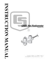
Section 1. Introduction1.1 RTDAQ Overview1.1.1 Main ScreenThe main screen of RTDAQ provides three tabs with datalogger interactionfunctions (Clock/Program, Monitor Data, and Collect Data), as well as atoolbar with buttons to launch frequently-used utilities and auxiliaryapplications.The toolbar includes utilities for working with data files (View Pro, Split, andCardConvert) as well as utilities for generating and editing dataloggerprograms (Short Cut, CRBasic, and the CR5000/CR9000X ProgramGenerator). Datalogger setup and status functions are also available, alongwith access to RTMC (Real-time Monitoring and Control) applications. Youcan also launch the Device Configuration Utility which is used to send newoperating systems to dataloggers and other peripheral devices, and to configuresettings in the dataloggers and other devices. All of the toolbar functionality isalso accessible from the RTDAQ menu, along with other tools, such as theTerminal Emulator, PakBus Graph, and LogTool (a program for viewingand storing communication logs). Each application includes extensive, onlinehelp.Some utilities installed with RTDAQ can be opened independently from themain RTDAQ program by using the Windows Start Menu item Programs |RTDAQ | Utilities. These utilities include the Device Configuration Utility(or DevConfig), View Pro, and CardConvert. DevConfig is describedabove. View Pro enables the viewing and graphing of collected data, andCardConvert converts data files originating from removable card storage intoother useful formats.1-2

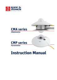
Section 1. Introduction1.1.2 Clock/Program and the EZSetup WizardSetting up the RTDAQ datalogger network is a relatively simple process withthe EZSetup Wizard, which guides you through the steps necessary to addand enter settings for dataloggers. Once a datalogger is added to the list, youcan choose the Edit Datalogger button to activate the Wizard again andchange those settings. Progress through the Wizard is shown on the left side ofthe screen, with steps for choosing a datalogger, defining the communicationspath between the computer and the datalogger, fine tuning settings for thedatalogger (e.g., baud rate or security code), testing communications, checkingor setting the clock, and finally sending a program or viewing a program filewhich is already running. After a datalogger has been added, you can selectand connect to that datalogger from the Clock/Program tab via point and clickoperations.1.1.3 Monitor DataOnce you’ve added and connected to a datalogger, the Monitor Data tabswitches to a view that lets you monitor the latest values measured on thedatalogger. You can monitor variables as they are updated after eachexecution of the datalogger program scan or monitor the latest data items thathave been stored into the datalogger’s tables.The Monitor Data tab also lets you edit public variables directly, or view datausing several available real-time monitors.1.1.3.1 Real-time MonitorsRTDAQ has a variety of windows for viewing datalogger data in near realtime.After the Monitor Data tab is selected, these options show as buttonswhich open separate windows when pressed.1-3

Section 1. Introduction• The status of ports, flags, or any boolean variables can be monitored andcontrolled within the Ports and Flags window.• The Table Monitor allows quick numeric viewing of entire output tables.• With both the Graph and Fast Graph, graphical data traces from adatalogger can be monitored in a window width as small as 1 millisecond,with resolution support for individual points up to 100 KHz.• The XY Plot allows up to four values to be plotted against anothermeasured value (other than the timestamp).• With the Fast Fourier Transform viewer, both single-valued (amplitudeor power spectrum) and dual-valued (real-imaginary or amplitude-phase)FFT spectra can be viewed.1-4

Section 1. Introduction• Histograms calculated by the datalogger can be shown as they are madeavailable by program calculations and storage.• Display of rainflow-style histograms is also supported using the Rainflowviewer. This display works with programs utilizing the Rainflow outputinstruction in the CRBasic datalogger program.1-5

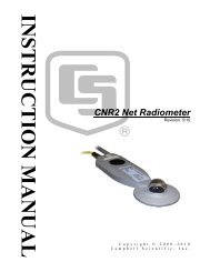
Section 1. Introduction1.1.4 Collect DataOnce a program is storing data in the datalogger you can collect a copy of thatdata to a file on the PC. The Collect Data tab shows a list of tables in thedatalogger as defined by the currently running program. You can retrieve theuncollected data, appending it to a file on the PC, or you can retrieve all of thedata from the datalogger. You can also use other custom configurations for thecollection. The Change File Name button lets you choose a folder and filename in which to store the data.1-6

Section 1. Introduction1.1.5 Field Calibration and the Calibration WizardRTDAQ includes the Calibration Wizard for performing real-time, nonintrusivecalibration of measurements. Datalogger programs that use theFieldCal CRBasic instruction activate this Wizard for use. This feature allowscalibration to occur within a simple interface, instead of requiring manualcalibration via the numeric displays or with the keypad display at thedatalogger site.1.1.6 RTMC Development, Run-time and Pro DevelopmentSeamless integration with the RTMC and RTMC Pro product line allowscreation of data monitoring and control screens for individual dataloggers.Custom screens are created using the RTMC Development programor theRTMC Pro Development program .1-7

Section 1. IntroductionExecution of these screens is done with the RTMC Run-time program. Bothprograms can be started using buttons from the main RTDAQ interface.The Standard RTMC Development and RTMC Run-time applications areincluded with RTDAQ. RTMC Pro must be purchased and installed separatelyfrom RTDAQ, but will operate within the RTDAQ environment afterinstallation.1.1.7 View ProRTDAQ includes View Pro, the “professional” version of CampbellScientific’s newly-updated data viewing application. View Pro lets youexamine data files (*.DAT files) collected onto the PC from the datalogger,and displays data in either comma-separated or tabular format, record byrecord. A graph can be displayed showing multiple traces (columns) of data.This program also allows the viewing of specialized data records such as FFTspectra and histograms.1-8

Section 1. IntroductionView Pro can be launched from a button on RTDAQ’s main screen. View Prois a simple analysis tool, and includes some basic printing and exportcapabilities.1.1.8 SplitSplit is a stand-alone application used to post-process data files on the PC andgenerate reports. A button on RTDAQ’s main screen launches the Split1.1.9 CardConvert1.1.10 Short Cutapplication . It can be used to merge data from multiple stations into onefile, perform calculations, and change date/time formats. Split can createreports or new files for input to other data analysis and display applications,including HTML formats.CardConvert is a utility to retrieve binary data from Compact Flash cardscontaining program output data, and convert the data to an ASCII file or otheruseful formats.Short Cut is a datalogger program “generator.” You select the dataloggertype, sensors, and desired outputs, and then Short Cut creates a simpleprogram file to send to the datalogger. Users don’t need to learn about theindividual programming instructions generated within the datalogger program.Short Cut includes support for multiplexers and a limited number of otherperipherals, and also provides a wiring diagram that you can print to leave inthe field with the datalogger.1-9

Section 1. IntroductionShort Cut is also an excellent way to learn about the CRBasic programminglanguage. The CRBasic programs created by Short Cut can be loaded directlyinto the CRBasic Editor for inspection or editing.1.1.11 CRBasic EditorThe CRBasic Editor is a program editor for CRBasic dataloggerprograms, including programs for the CR800, CR850, CR1000, CR3000,CR5000, and CR9000X. It is used to manually create programs or to editexisting or generated programs.Program instructions are defined within the editor for variable declarations,data table configuration, measurements and control operations, numericprocessing, logical operations, data output, and program control. Extensiveassistance and program examples are provided in the online help system.1.1.12 CR5000/CR9000X Program GeneratorsRTDAQ includes updated versions of the program generators for theCR9000X and CR5000which were previously available in PC9000.1-10

Section 1. IntroductionCR9000X and CR5000 programs can be generated using a detailed,instruction-level interface resulting in extensive control over generatedprograms.1.2 Getting Help for RTDAQ Applications1.3 Windows ConventionsDetailed descriptions of each application or tool are included in later sectionsof this manual. Each application also has its own built-in help system.Context sensitive help for an application can usually be accessed by movingthe focus to (i.e., clicking on) a particular item and pressing the F1 key or byselecting Help from the application's menu.Contact your Campbell Scientific representative if you are unable to resolveyour questions after reviewing the above noted resources.There are numerous conventions and expectations about the way a softwareprogram looks and behaves when running under Microsoft Windows.Campbell Scientific has adopted many of these conventions in RTDAQ.This manual describes a collection of screens, dialogs, and functions tointeroperate with Campbell Scientific’s dataloggers. As with most Windowsbasedsoftware there is usually more than one way to access each function. Weencourage you to look around and experiment with different options to findwhich methods work best for you.To keep this manual as concise and readable as possible, we will not alwayslist all of the methods for getting to every function. Typically each functionwill have two methods of access and some will have as many as four.1-11

Section 1. IntroductionThe most common methods for accessing functionality are:Menus – Text menus are displayed at the top of most windows. Menu itemsare accessed either by a left mouse click, or using a hot key combination (e.g.,Alt+F opens the File menu). When the menu is opened, you can click on anitem to select it, or use arrow keys to highlight it and press the Enter key, orjust type the underlined letter.By convention, menu items that bring up dialog boxes or new windowsrequiring interaction will be followed by an ellipsis (…). Other items executefunctions directly or can be switched on or off. Some menu items show acheck mark if a function is enabled and no check mark if disabled.Items with Program Focus – On each screen one button, text area, or othercontrol is selected at a time to “have the focus.” The “Focus” is usuallyindicated when the item is surrounded by a dotted line or is bolded. Pressingthe tab key can move the focus from item to item. Typing text changes aselected text edit box that has the focus. Pressing the space bar toggles aselected check box. A selected button can also be activated by pressing theEnter key.Buttons – Buttons are an easy way to access a function. They are normallyused for the functions that need to be called frequently or are very important.Clicking a button executes that function or brings up another window. Buttonfunctions can also be accessed from the keyboard using the tab key to moveamong items on a screen and pressing the Enter key to execute the buttonfunction. Most text-based buttons have a hot-key.Right-Click Menus – Some areas have pop-up menus that bring up frequentlyused tasks or provide shortcuts. Just right-click on an area and if a contextmenu appears, left-click the menu item you want.Hot Keys or Keyboard Shortcuts – Many of the menus and buttons can beaccessed using Hot Keys. An underlined letter identifies the hot key for abutton or function. To get to a menu or execute a function on a button holddown the Alt key and type the underlined letter in the menu name or the buttontext. The hot key letters may not appear until after you’ve pressed the Alt key.Pop-Up Hints – Hints are available for many of the on-screen controls. Letthe mouse pointer hover over a control, text box or other screen feature and thehint will appear automatically and remain visible for a few seconds. Thesehints will often explain the purpose of a control or a suggested action. For textboxes where some of the text is hidden, the full text will appear in the hint.1-12

Section 2. System Requirements2.1 Hardware and SoftwareRTDAQ is an integrated application of 32-bit programs designed to run onIntel-based computers running Microsoft Windows operating systems.Recommended platforms for running RTDAQ include Windows XP, WindowsVista, and Windows 7.RTDAQ also requires that TCP/IP support be installed on the PC.2-1

Section 2. System Requirements2-2

Section 3. Installation, Operation andBackup Procedures3.1 CD-ROM InstallationThe following instructions assume that drive D: is a CD-ROM drive on thecomputer from which the software is being installed. If the drive letter isdifferent, substitute the appropriate drive letter.1. Put the installation CD in the CD-ROM drive. The install applicationshould come up automatically. Skip to step 3.2. If the install does not start, then from the Windows system menu, selectStart | Run. Type “d:\setup.exe” in the Open field or use the Browsebutton to access the CD-ROM drive and select the setup executable. Thisactivates the RTDAQ Installation Utility.3. Follow the prompts on the screen to complete the installation. Theinstallation will require a CD key. You will find this code printed on theback of the jewel case of the original installation CD.A shortcut to launch RTDAQ is added to your computer’s Start menu underPrograms | Campbell Scientific | RTDAQ. If the default location is used,RTDAQ executable files and help files are placed in the C:\ProgramFiles\CampbellSci\ directory (folder), with the main RTDAQ applicationlocated in the C:\Program Files\CampbellSci\RTDAQ directory.Working directories will also be created in the C:\Campbellsci directory forRTDAQ’s configurations and data files, user programs, and settings for theaccessory applications and utilities.Trial VersionIf you are installing the trial version of RTDAQ, you will have 30 days to usethis fully functional trial version. Each time you run RTDAQ, you will beadvised as to how many days are remaining on your trial version. At the endof the 30 days, the trial version of RTDAQ will no longer function.If you choose to purchase RTDAQ, you will need to run the install program onthe RTDAQ CD and input the CD Key from the back of your CD case. Thiscan be done either before or after the 30-day trial period has expired.Note that the trial version will install some applications in theC:\Program Files\Campbellsci\Demo directory. When the purchased versionof RTDAQ is installed, these applications will each be installed in their owndirectory under C:\Program Files\Campbellsci. The versions in the Demodirectory will no longer be used. Therefore, to avoid having these unusedversions remain on your computer, you may wish to uninstall the trial versionbefore installing the purchased version of RTDAQ.3-1

Section 3. Installation, Operation and Backup Procedures3.2 RTDAQ Operations and Backup ProceduresThis section describes some of the concepts and procedures recommended forroutine operation and security of the RTDAQ software. Since the occurrenceof operational issues cannot be fully eliminated on most computer systems, thefollowing guidelines and procedures are provided to help minimize possibleproblems that may occur.3.2.1 RTDAQ Directory Structure and File Descriptions3.2.1.1 Program Directory3.2.1.2 Working DirectoriesAs described earlier in the installation procedures, the files for programexecution are stored in the C:\Program Files\Campbellsci\ directory. Thisincludes the executables, DLLs, and most of the application help files. Thisdirectory does not need to be included in back up efforts. RTDAQ and itsapplications rely on registry entries to run correctly; therefore, any restorationof the program should be done by reinstalling the software from the originalCD.In this version of RTDAQ, each major application keeps its own workingdirectory. The working directory holds the user files created by theapplication, as well as configuration and initialization (*.INI) files.This scheme was implemented because Campbell Scientific uses theunderlying tools and many of the applications (the communications server,library files, datalogger program editors, etc.) in a number of differentproducts. By providing a common working directory for each majorapplication, you should see consistent file organization as you move from oneproduct to another.3-2

Section 3. Installation, Operation and Backup ProceduresThe following figure shows the typical working directories for RTDAQ if thedefault options were selected during installation:FIGURE 3.2-1. Typical Working Directories for RTDAQ3.2.2 Backing up the Network Map and Data FilesAs with any computer system that contains important information, the datastored in the RTDAQ working directory should be backed up to a securearchive on a regular basis. This is a prudent measure in case the hard diskcrashes or the computer suffers some other hardware failure that preventsaccess to the stored data on the disk.The maximum interval for backing up data files collected from dataloggersdepends primarily on the amount of data maintained in the datalogger memory.The datalogger’s data tables are typically configured as ring memory. Recordswill be stored to a table until the number of records reaches a predefined size,and then each new record will overwrite the oldest record. If the data isbacked up more often than the oldest records in the datalogger are overwritten,a complete data record can still be maintained by restoring the data from thebackup and then re-collecting the newest records from the datalogger.3-3

Section 3. Installation, Operation and Backup Procedures3.2.2.1 Performing a BackupRTDAQ provides a simple way to back up the network map, the RTDAQ datacache, and the initialization files for the main application. The network mapwill restore all settings and data collection pointers for the dataloggers andother devices in the network. The data cache is the binary database whichcontains the collected data from the datalogger. Initialization files store settingssuch as window size and position, configuration of the data display, etc.NOTEThe *.INI files backed up in the RTDAQ backup procedure arethose found in the C:\Campbellsci\RTDAQ\sys\inifiles folderonly. Other *.INI files such as those for Short Cut,CardConvert, Split and the CRBasic Editor are not a part of thebackup.From RTDAQ’s menu, choose Network | Backup/Restore Network, and thenpress Backup.The backup file is named RTDAQ.bkp and is stored in theC:\CampbellSci\RTDAQ directory (if you installed RTDAQ using the defaultdirectory structure). You can, however, provide a different file name ifdesired.3.2.2.2 Restoring the Network from a Backup File3.2.3 Loss of Computer PowerTo restore a network from a backup file, choose Network | Backup/RestoreNetwork. Select the *.bkp file that contains the network configuration youwant to restore, and press Restore. Note that this process DOES NOT appendto the existing network — the existing network will be overwritten when therestore is performed.The RTDAQ communications server writes to several files in the \SYSdirectory during normal operations. The most critical files are the data cachetable files and the network configuration files. The data cache files contain allof the data that has been collected from the dataloggers by the RTDAQ server.These files are kept open (or active) as long as data is being stored to the file.The configuration files contain information about each device in the dataloggernetwork, including device settings, and other parameters. These files arewritten to frequently to make sure that they reflect the current state andconfiguration of each device. The configuration files are only opened asneeded.If computer system power is lost while the RTDAQ server is writing data tothe active files, the files can become corrupted, making the files inaccessible tothe server. While loss of power won’t always cause a file problem, havingfiles backed up as described above will allow you to recover more effectivelyif a problem occurs. If a file does get corrupted, all of the server’s workingfiles need to be restored from a backup file to maintain synchronization withthe server state.3-4

Section 4. The RTDAQ Main ScreenThis section provides an overview of RTDAQ, including a detailed description of thecommunications tabs, pull-down menus, and toolbar. An overview of RTDAQ’stroubleshooting tools is also provided.4.1 Overview4.1.1 Program Startup and Main Screen FunctionalityTo start RTDAQ go to the Start menu of the computer and select the RTDAQicon under Start | Programs | Campbell Scientific | RTDAQ. You can also usethe shortcut on the desktop if you elected to create one during the installationprocess.Setting up and configuring RTDAQ to communicate with dataloggers is donewith the EZSetup Wizard. This Wizard appears automatically the first timeyou run RTDAQ. To add additional dataloggers, click the Add Dataloggerbutton on the main toolbar to bring up the EZSetup Wizard again. Theediting of existing dataloggers and their communications settings is also donethrough this Wizard, through use of the Edit Datalogger button .RTDAQ offers an integrated main screen, with three tabs for basiccommunications functions (Clock/Program, Monitor Data, and CollectData), and buttons from which to launch auxiliary applications to work withdata files or create datalogger programs.4-1

Section 4. The RTDAQ Main ScreenThe RTDAQ main screen consists of a Title Bar, Menu Bar, Toolbar,Datalogger Network Map, Clock/Program tab, Monitor Data tab, CollectData tab, and Status Bar as shown here:The Title Bar shows the RTDAQ application name and version, as well as thedatalogger station name and model name currently highlighted for selection orconnection. The Menu Bar, Toolbar, Clock/Program tab, Monitor Data tab,and Collect Data tab are described in more detail later in this chapter.The Network Map shows which loggers have been configured for connectionwithin the system. You can connect to a datalogger by double-clicking on itsicon, or by selecting it and pressing the Connect button on the Toolbar.RTDAQ connects to only one datalogger at any one time. The Status Bar isused to show the current connection status (and connection time if connected)for the selected datalogger.RTDAQ provides additional tools for working with your dataloggers and data.RTMC support is provided for viewing live data in a customized display.Split, View Pro, and CardConvert are used to examine and process data files.Short Cut and the CR5000/CR9000X Program Generator (ProgGen) can beused to generate datalogger programs, and the CRBasic Editor is provided formore advanced datalogger program editing. DevConfig is used to configuresettings in dataloggers and other peripheral devices. These tools are accessed4-2

Section 4. The RTDAQ Main Screenvia the buttons on the main screen or the pull-down menu selections under theTools menu. More information about these tools is provided later in thismanual.4.1.2 Datalogger Connectivity, Help and Program Exit4.2 EZSetup Wizard4.2.1 Add DataloggerRTDAQ supports the major CRBasic dataloggers, including the CR800,CR850, CR1000, CR3000, CR5000, and CR9000X.RTDAQ supports one medium of communications for any given datalogger.These media include direct connect via serial communications (or RS-232) vialocal serial cable, short haul modems, other “transparent” links, telephone,TAPI, TCP/IP, VHF/UHF radios, RF400-series spread spectrum radios, andmultidrop interfaces (MD9 and MD485).RTDAQ does not support parallel port communications, RF95T modems, ormultiple media (such as phone-to-RF). RTDAQ is designed to use PakBusdataloggers and other PakBus devices in their default configurations; they arenot supported as PakBus routers.In order to be easy to use, RTDAQ relies on user-attended communications. Itdoes not provide for automated scheduled data collection or automated clockchecks. It does not support remote connections from other PCs.Help for each application is available from the Help menu item, or by movingthe focus to a control (by clicking on or tabbing to a control) and pressing F1.To exit RTDAQ, either click the [X] in the upper right hand corner of the mainscreen, or select Exit under the File menu.Dataloggers are added to the network with the EZSetup Wizard. This Wizardis also used to edit the settings for a datalogger after it’s been added. TheEZSetup Wizard is automatically displayed when RTDAQ is run for the firsttime.When RTDAQ is not connected to a datalogger, you may add a datalogger toyour network map by selecting the Add Datalogger button or by choosingNetwork | Add Datalogger from the menu. The EZ Setup Wizard will appearallowing you to select and configure your new datalogger.4-3

Section 4. The RTDAQ Main ScreenPrevious and Next buttons are provided for easy movement through theWizard. Progress is shown by the blue arrow next to each step displayed on theleft of the screen. Help is available from the Help button as well as the textdisplayed on the right side of the screen.4.2.2 Communication Setup4.2.3 Datalogger SettingsIn the Communication Setup step you select the datalogger type and give it aname that will also become the default file name for data files collected fromthat datalogger. You may set up connections for the following loggers:CR9000X, CR5000, CR1000, CR3000, and the CR800 Series (which includesboth the CR800 and CR850). The next step allows you to choose from thecommunications media that are available for the datalogger. RTDAQ willdisplay the serial ports (COM ports) known to your Windows operatingsystem. RTDAQ fills in as many communications settings as possible and inmany cases you can use the default settings. It provides fields for user-enteredcommunications settings such as phone numbers and RF radio addresses. Helpfor entering these settings is provided on the right side of each screen, byclicking the F1 key, or by pressing the Help button for each wizard screen.You may also want to consult the manual corresponding to the particularcommunications hardware you are configuring.The Datalogger Settings step is provided for fine tuning the connection to thedatalogger. The baud rate offered is typically the maximum baud ratesupported by that datalogger and communications medium; lower rates may berequired for cell phones or noisy telephone links. Enter a Security Code onlyif the datalogger is configured – via the keyboard/display or settings in thedatalogger program – to use it.4-4

Section 4. The RTDAQ Main Screen4.2.3.1 Max Time OnlineNote that the default Max Time On-Line setting for most communicationslinks is zero (“0 d 00 h 00 m”), which means that RTDAQ will never hang upuntil you click Disconnect. For telephone links, the default Max Time On-Linesetting is 10 minutes in order to reduce the possibility of inadvertent andexpensive long distance or cellular telephone charges. There are, however,other links that can result in expensive connection charges, such as digitalcellular links using TCP/IP that charge by the byte. Leaving the dataloggerconnected also uses battery power, so if the datalogger power supply is notrecharged from a reliable source, it may discharge its battery below safe levels.Be sure, therefore, that you do not leave the datalogger connected beyond thetime necessary to do the tasks you need to do.4.2.4 Summary, Communications Test, and Clock Set4.2.5 Send ProgramThe Setup Summary step provides a list of the settings entered. You can usethe Previous button to go back and change settings as necessary.The Communications Test step allows you to test the communications linkbefore going any further. If the datalogger is not installed, you can skip thisand the next two steps.If communication succeeds, you can move to the Datalogger Clock step whereyou can check or set the datalogger’s clock to match the PC’s system time. Ifthe datalogger is in a different time zone, you can enter an offset in hour andminutes.The Send Program step allows you to send a program to the datalogger. Thismay be a program you created with Short Cut, ProgGen, the CRBasic Editoror a program supplied by someone else. Dataloggers will display the programname if one is running and will provide table definitions that contain datalabels. If you don’t have a program for the datalogger you can skip this stepand send a program later from the Clock/Program tab.If you connected to the datalogger during the EZSetup Wizard, when you leavethe Wizard it will ask if you wish to stay connected.4.2.6 Editing and Deleting DataloggersOnce you’ve added a datalogger, you may disconnect and use the otherdatalogger configuration buttons on the Toolbar to delete that datalogger, editits settings, or add another datalogger to the Network Map.4-5

Section 4. The RTDAQ Main Screen4.3 Clock/Program Tab4.3.1 Basic OperationSelection of the Clock/Program tab brings up the Clock/Program screen.RTDAQ displays this tab by default when first executed.In this screen you can see brief details about the currently selected datalogger,including its name in the Network Map, its station name, its connectioninformation, and its response time settings. When connected, you can alsoview the current time as given by the datalogger, as well as the time given bythe PC’s clock. You can set the clock on the datalogger to be synchronizedwith the PC clock. You can also view the name of the current programrunning on the datalogger. You can send a program or operating system to thedatalogger. You can also retrieve the currently running program to your PC.4-6

Section 4. The RTDAQ Main Screen4.4 Monitor Data TabOnce you’ve added and connected to a datalogger, you can monitor the valuesstored by the datalogger in real-time. Choose the Monitor Data tab to displaythe Monitor Data screen.4.4.1 Field MonitorThis screen contains the Field Monitor, which displays values from dataloggertables, including stored tables and the public table. Press the Add button tobring up a screen for selecting data table fields to be monitored in this screen.After the Start button has been pressed, RTDAQ will display the last recordstored to that table and will automatically update these records as they arestored in the datalogger’s memory. Note that RTDAQ does not automaticallystore this data to a data file on the PC. If you want a permanent record of thedata, you must collect it manually from the Collect Data tab.You may find that your labels or the number of digits displayed are too long tofit in the space provided. Using the mouse, you may put your cursor over theborder between the columns for the labels and values and drag it left or right tomake it easier to read. The column width is not preserved when RTDAQ isclosed and restarted. The table name, variable name and data value also willbe displayed momentarily as a popup hint if you hover your cursor over avalue for a few seconds.4.4.2 Editing Variable ValuesIn some cases, you may wish to edit public variables. For example, you maychoose to change sensor offsets or control variables affecting dataloggerprogram execution. To change public variable values, double-click on the4-7

Section 4. The RTDAQ Main Screennumber itself until it turns yellow, then use the PC keyboard to enter a newvalue. Alternately, you can right-click the value, select View/Modify Value,and edit the value in the resulting dialog box.4.4.3 Specialized Real-time Monitor Screens4.5 Collect Data TabThe Monitor Data screen is also used to access the specialized real-time datamonitor screens. For more information about the Monitor Data screen, seeChapter 7 “Monitoring Data in Real-time”.To retrieve a copy of the data from the datalogger and store it permanently intoa file located on your PC, select the Collect Data tab.The Collect Data screen allows for manual data collection. The mode for thedata collection is specified, as well as whether the collected data should bestored in a new output file or appended to an existing one. The format of theoutput file is also selected.To collect a range of data from a specified timeframe, you can use the StartingDate/Time and Ending Date/Time options. Choices for including timestampsand record numbers in the stored data are also included. A choice of tables tobe collected for output is given. Tables can be selected individually or as agroup.The station name identifier can be chosen to be included in the header of thedata file if desired. Names and paths for the output files can be selected asdesired. Finally, the collection is initiated using the Start Collection button.For more information about this screen refer to the associated online helptopic.4-8

Section 4. The RTDAQ Main Screen4.6 Pull-down MenusAccess to almost all of the buttons and tabs on RTDAQ’s screens is alsoavailable via pull-down menus. Many of these functions are described in detailin other sections of this manual.The File menu is used to save and retrieve global setting configurations andclose the RTDAQ program. The View menu allows selection of languagesother than English. The Datalogger menu is used for datalogger controlfunctions, connections, and wizards. The Network menu is used for adding,editing and deleting loggers, and performing backups of the network map. TheTools menu is used for accessing supplementary programs such as the onesshown on the Toolbar. The Help menu is used for accessing the RTDAQonline help system.4.6.1 File Menu4.6.1.1 Saving and Loading ConfigurationsFor information on how to use these functions, refer to the “Saving andLoading Global Configuration Files” section of Chapter 7 “Monitoring Data inReal-Time”.4.6.1.2 ExitThe Exit item is used to close all real-time windows, disconnect from theconnected datalogger, and close RTDAQ.4.6.2 View MenuRTDAQ can display the user interface component text (for buttons, dialogboxes, and other user interface elements) in a language other than English if aseparate language package has been installed. If a language package isinstalled on your machine, the View menu will have a Languages entry andyou will see the installed language as an item in the submenu. When a newlanguage is chosen, RTDAQ will immediately reflect that change. Openedclients will not reflect the change until they are closed and reopened.Applications that support alternate languages are Short Cut, CRBasic Editor,View Pro, CardConvert, PakBus Graph, LogTool, and the DeviceConfiguration Utility.NOTEAvailable language packages are provided by CampbellScientific's international representatives or on the CSI web site.They are not included in the standard RTDAQ installation.4-9

Section 4. The RTDAQ Main Screen4.6.3 Datalogger Menu4.6.3.1 Connect/Disconnect4.6.3.2 Update Table DefinitionsThis option provides the same function as the Connect/Disconnect button onthe main toolbar (see Section 4.7).When a CRBasic datalogger is configured for the first time or when a newprogram is sent, RTDAQ queries the datalogger for its table definitions.Whenever a new program is loaded into the datalogger, the table definitionswill automatically be sent to RTDAQ. When using the real-time screens toview data, RTDAQ requires the latest table definitions in order to workproperly. To avoid unnecessary data throughput on a datalogger, thisinformation is not sent to RTDAQ with every configuration change, but onlywhen deemed necessary, such as when a program changes.If you find the table definitions in RTDAQ to be mismatched with thedatalogger program, you can update those definitions manually. To update thetable definitions for a datalogger manually, connect to that datalogger andselect Update Table Definitions from the Datalogger menu.4.6.3.3 Status TableCRBasic dataloggers include a default data table called the Status Table, whichdisplays key values about the condition of the datalogger. The Datalogger |Status Table menu item opens a window to display that information. Recordsfrom the datalogger’s status table are generated on demand. Each dataloggerhas its own list of status fields, but they typically include such information asthe hardware operating system version, the name of running program, batteryvoltage, various error counters including watch dog and low batteryconditions, and an estimate of how many days it will take for data tables tobegin overwriting their oldest records. Detailed information on the status tablefor each datalogger can be found in the operator’s manual for that particulardatalogger.4-10

Section 4. The RTDAQ Main ScreenThe Status Table display screen is shown below:This window has three tabs: Summary, Table Fill Times, and Status Table.4.6.3.3.1 Summary TabThe Summary tab provides an overview of important status information fromthe datalogger, including information about the datalogger model and itsfirmware, current program details including error information (if any), batteryvoltage levels, and card memory (if one is present). Press the Refresh buttonto prompt RTDAQ to query the datalogger and update the values, the Savebutton to save the information being displayed to a file, or the Print button toprint the information being displayed.4-11

Section 4. The RTDAQ Main Screen4.6.3.3.2 Table Fill TimesThe Table Fill Times tab lists the tables in the datalogger, along with themaximum number of records the table can hold, the estimated amount of timethat it will take the table to fill, and the estimated date and time that the tablewill fill based on the time the datalogger program was downloaded and thetable size. This fill information helps the user determine the collectionschedule that should be performed on the datalogger. Data should be collectedno less frequently than a user can afford to lose it. A data table can be resetfrom this window by pressing the Reset Tables button.Press Refresh to prompt RTDAQ to query and update the values.NOTEResetting a table will erase the data in the datalogger and in thedata cache.4.6.3.3.3 Status Table TabThe Status Table tab lists all of the status table fields in the datalogger alongwith their values. By default, all of the fields in the status table are displayed.To select only certain status data to be viewed, press the Select Fields button.This will display a list of the status fields available in the datalogger. Selectone or more of the fields and then press OK. The current values will bedisplayed in the table. If you select a cell within the status table and rightclick, a short cut menu will be displayed. From this menu you can SelectFields or View/Modify a value (if it is a writable value).Press the Refresh button to prompt RTDAQ to query the datalogger andupdate the values, the Save button to save the information being displayed to afile, or the Print button to print the information being displayed.4.6.3.4 File ControlThe dataloggers used in RTDAQ have a built in file system much like acomputer hard disk. Multiple files can be stored in the datalogger's memory oron a PC card, including data files, calibration files, and datalogger programs.The dataloggers retain files in memory unless they are specifically deleted orremoved as part of a program change operation.The File Control window is used to manage all the files on the dataloggers.The Datalogger | File Control menu item opens File Control.4-12

Section 4. The RTDAQ Main Screen4.6.3.4.1 Datalogger DevicesEach datalogger will have a device designated as the CPU drive. If an add-incard is installed on the datalogger, you will also see the CRD storage device.The File Control window displays a list of files stored on each of its devicessuch as the CPU, PC card, or user-specified drive. The window on the left listsall of the data storage devices available for the selected datalogger (CPU,CRD, or USR). Selecting a device shows a list in the right pane of the screendisplaying the files stored on that device.NOTEThe USR drive is a user-created drive in the CR800, CR1000,and CR3000 dataloggers. It can be set up by assigning a value tothe datalogger's UsrDriveSize setting in the status table. Thisdrive must be set to at least 8192 bytes, in 512 byte increments.If the value entered is not a multiple of 512 bytes, the size willbe rounded up. The size may also be rounded up to the accountfor a certain amount of overhead that is required for the drive tooperate.4.6.3.4.2 Run OptionsThe Run Options for a program file indicate whether it is set to Run Now,Run On Start-up, or both (Run Always). The currently executing program isindicated by the Run Now or Run Always attribute. The file size is alsodisplayed for each file, as well as the last time the file was modified andwhether or not the file is Read Only or Read/Write. Note that the Size andModified date are not available for the CR9000X and CR5000 dataloggers.4-13

Section 4. The RTDAQ Main Screen4.6.3.4.3 Working with Files and DirectoriesThere are several options for working with the files and directories on thedatalogger.Send is used to transfer files from the computer to the datalogger. Clicking theSend button brings up a standard file selection dialog box. A new file can bechosen and sent to the highlighted device. Datalogger programs, data files,and other ASCII files can be sent to the datalogger.If you select the Set Run Options on Send check box in the File Controlscreen, you will have the opportunity to set the Run On Power-up and/or RunNow options as the file is being transferred from the PC’s file system to theselected device (see the Run Options section below).Format is used to format the selected device. Just like formatting a disk on acomputer, all of the files on the device are deleted and the device is initialized.Refresh will update the list of files for the selected device.Retrieve will get the selected file from the datalogger and store it on thecomputer. A Save As dialog box comes up allowing you to specify thedirectory and file name for the saved file.Run Options brings up a dialog box that is used to control what program willbe run in the datalogger. Highlight a file, and then select the Run Optionsbutton.Run Now will stop the program currently running on the datalogger and thenload and run the selected program. During this process, all of the existing datatables in datalogger memory are deleted. If data is also being stored to a card,select an option button to determine whether or not the data tables created bythe program and stored on the card are to be erased or retained.To use the Erase all card data files option when sending a program to aCR9000X or CR5000 datalogger, you must send the program to the dataloggerfirst without starting it, and then select the Run Options on the program fromthe File Control screen. You can then start the program and select the Eraseoption or the Do Not Erase option. With the CR1000 and CR30004-14

Section 4. The RTDAQ Main Screendataloggers this setting can be selected when the program is sent to thedatalogger.Run On Power-up sets the file to run when the datalogger is powered downand powered back up.A file set to Run Now and Run On Power-up will be shown as Run Alwaysin the File Control window.Delete - Highlight a file and press the Delete button to remove the file from thedatalogger's memory. A running program may not be deleted.Stop Program halts execution of the currently running datalogger program.For all dataloggers but the CR800, CR1000, and CR3000, note that all datatables will be deleted when the program is stopped. For a CR800, CR1000, orCR3000 select the option to stop the program and retain the data files, or tostop the program and erase all data files.If a CR800, CR1000, or CR3000 program has been stopped, use the RunOptions to restart it. Once again, you will be able to choose whether to retainor erase the data files. You can also choose a new program file to run.4.6.3.4.4 Right-Click Menu OptionsWhen a file name is selected, pressing the right mouse button displays a menuwith the Retrieve File, Delete File, Rename File, Run Options, and StopProgram options.4.6.3.5 Calibration WizardThis item can be used to calibrate measurements being made by the currentlyconnected datalogger. The program in the datalogger must be written with theproper instructions to enable these calibrations.For complete information on how to activate and use the Calibration Wizard,see Section 9 “Calibration and Zeroing”.4-15

Section 4. The RTDAQ Main Screen4.6.3.6 Terminal EmulatorTerminal Emulator emulates a terminal connected to a datalogger orcommunications device. Terminal Emulator comes up showing a blankscreen. Clicking on Select Device shows a list of devices known to RTDAQ.Selecting a device and baud rate, and then clicking Open Terminal causesRTDAQ to attempt to connect with that device. If the device is a datalogger,RTDAQ will call the datalogger over whatever communications link has beenestablished and will attempt to get a prompt from that datalogger. If the deviceis a root device, such as a serial or COM port, RTDAQ simply opens that portat the specified baud rate.Terminal Emulator has several uses. If you open a COM port, you can use it toset up devices that present their own menus, such as RF400 radios or NL100s.See the manuals for those devices to obtain information on how to navigate themenus and what settings to choose.Another potential use is to communicate with smart devices attached to thedatalogger. Some dataloggers allow a “pass-through” mode whereby you cancommunicate through them to an attached SDI-12 sensor to set its address orother parameters. See the manuals for the datalogger and sensor for therelevant commands.Troubleshooting communications devices is another use for TerminalEmulator. When calling for support on these devices, an applications engineer4-16

Section 4. The RTDAQ Main Screenmay ask you to use this method to manually dial through phone or RFmodems, for example.You can close a connection to start another one by clicking the CloseTerminal button. You can close the Terminal Emulator itself by clicking the[X] button in the upper right corner of the screen.4.6.4 Network Menu4.6.4.1 Add/Delete/Edit/Rename DataloggerThe Add Datalogger, Delete Datalogger, and Edit Datalogger Setup optionsperform the same functions as the buttons on the main toolbar. The RenameDatalogger item can be used to change the name of a datalogger.4.6.4.2 Backup/Restore NetworkThis function can be used to save a copy of the network map to a file, and thento restore the network if necessary. The settings for all the devices in thenetwork will be saved.A default is given for the directory and file name to be used for the backup orrestore. This can be changed by typing over the default directory and/or filename or selecting the button to the right of the field containing the file nameand browsing to the desired directory and file name.To backup the current network map, select the file name to which the backupwill be stored, and then press the Backup button. The network map will besaved to the chosen file, and a message will appear indicating that the networkhas been backed up.To regenerate the network map from a backup file, select the name of thebackup file to restore from the dialog box, and then press the Restore button.Note that this backup will replace the existing network (it does not add to theexisting network).The backup/restore option will be disabled if you are currently connected to adatalogger. You must disconnect from the datalogger before performing abackup or restoring the network.4.6.4.3 Computer’s Global PakBus AddressRTDAQ communicates with the CR1000, CR3000 and CR800 seriesdataloggers using the PakBus protocol. All nodes and routers, includingdataloggers and the computer itself in a PakBus network must have a uniquePakBus address less than 4095 (and typically less than 4000). Setting up aPakBus network that communicates between the nodes can be a complex task,so RTDAQ avoids complexity by setting up each PakBus datalogger within itsown PakBus subnetwork. RTDAQ uses a PakBus “Port” with a uniquePakBus address to receive communications from PakBus devices. Setting thisglobal address will cause each new PakBus datalogger added to the NetworkMap to connect to RTDAQ using the specified PakBus address.4-17

Section 4. The RTDAQ Main ScreenThe CR800/850, CR1000 and CR3000 dataloggers keep track of the PakBusaddresses of other devices that communicate with them, including PCs. Ifmore than one PC is communicating with a single PakBus datalogger, it maybe helpful to assign each PC its own PakBus address. PakBus addressesgreater than 3999 are reserved for PCs or routers. Address 4095 is reservedfor broadcast messages. Keep in mind that, although PakBus devices keeptheir own routing tables, they will communicate with any other PakBus devicethat has an address >3999. Therefore, you may want to use different PakBusaddresses for each PC communicating with your PakBus dataloggers. RTDAQuses address 4090 by default, LoggerNet uses 4094, PC400 uses 4093,PC200(W) uses 4092, and 4091 is used by CSI’s PDA software. This menuitem provides the ability to change that computer level address.4.6.5 Tools Menu4.6.5.1 Auxiliary ApplicationsUse the items on the Tools menu to launch the auxiliary programs, includingthe RTMC applications, View Pro, Split, CardConvert, Short Cut, CRBasicEditor, and the CR5000/CR9000X Program Generator (ProgGen). Someusers prefer using the keyboard instead of the mouse. The Alt-T keystroke isprovided to facilitate keyboard access. These applications are described inmore detail later in this manual as described below:RTMC Development, RTMC Pro Development, RTMC Run-time: SeeSection 8: Real-Time Monitoring and Control SoftwareViewPro: See Section 6: ViewProSplit: See Section 10.3: SplitCardConvert: See Section 10.1: CardConvertShortCut: See Section 5.2: Short CutCRBasic Editor: See Section 5.1: CRBasic EditorProgGen: See Section 5.3: Program Creation with the RTDAQ ProgramGeneratorDevice Configuration Utility: See Section 10.2: Device Configuration Utility4-18

Section 4. The RTDAQ Main Screen4.6.5.2 OptionsThe following two options can be set to control the general operation ofRTDAQ:Automatically Check Datalogger Status - This option allows you todetermine when the datalogger status table is automatically checked. Theoptions include After Connection, After Program Send, and/or On Interval.The status values checked include the following: PakBus Address, WatchDogErrors, Skipped Scans, Skipped Slow Scans, Skipped Records, Variable Out ofBounds, Program Errors, Battery Voltage, Lithium Battery, Number of timesvoltage has dropped below 12V, Number of times voltage has dropped below5V, Stack Errors, and Calibration Errors. Note that not all status values areapplicable to all dataloggers. Only those status values applicable to the currentdatalogger will be checked.If a problem is found during a datalogger status check, the status table will popup along with a warning indicating the problem that has been identified.Show Hints - The Show Hints option is used to turn on/off the tool tips thatappear when your mouse hovers over a control (button or field). When acheck mark appears beside the menu item, the tool tips will be displayed.When the check mark does not appear beside the menu item, no tool tips willbe displayed. This menu item is a toggle; select it to change its state.4.6.5.3 LogToolSooner or later every communications link will experience some problems.Sometimes these problems resolve themselves, such as when phone lines arebusy at first, but become available as other users complete their tasks.When the resolution of communications problems is not straightforward, theLogTool application can allow detailed analysis of communications activity.LogTool is accessed from the Tools | LogTool menu item.4-19

Section 4. The RTDAQ Main ScreenOn the left side of the LogTool window is a display of all devices set up inRTDAQ. You can choose to show all messages or filter them to show onlycertain devices or dataloggers. RTDAQ can also store these messages to logfiles on the PC’s hard drive and will eventually overwrite these files to keepthem from growing forever. You can control whether these logs are used, aswell as the number and size of each log file type with the Options | Log FileSettings menu and dialog.RTDAQ’s communications engine creates four different types of messagelogs. Transaction messages are the highest level, and show every actionundertaken by RTDAQ. For example, if you’re monitoring a datalogger everysecond, RTDAQ will show clock check messages each second. Many of themessages displayed on this log are understandable and may provide someinsight to the processes going on behind the scenes when you monitor orcollect data.The other three logs are more technical in nature, but can be very useful toCampbell Scientific support engineers. Communications messages show whendevices are activated, the settings passed to those devices, and their responses.This log may include status, warning, and fault messages. The Object Statemessages record the state of software objects behind the scenes in RTDAQ.The most detailed log is the Low Level Log. A separate log is stored for eachroot level device (each COM port, IP port or TAPI port). These logs recordevery byte sent or received through that port. Interpreting all of these logsrequires knowledge of both Campbell Scientific protocols as well as other,lower level protocols, and requires a detailed understanding of what is4-20

Section 4. The RTDAQ Main Screensupposed to be happening. Most users will only need to access these logswhen requested to do so by Campbell Scientific support personnel.For more information about the content of these logs see Section 10.4.6.5.4 PakBus GraphPakBus Graph is a utility that graphically depicts the connections in a PakBusdatalogger network. It provides a look at RTDAQ's PakBus routing table. Inaddition, the utility can be used to change the settings of a PakBus device.The window for PakBus graph is divided into three sections: the list of PakBusdevices, a graphical depiction of the PakBus network, and the log messages forPakBus communications. The list of devices and the log can be toggled off byclearing the Show List View and Show Log options, respectively.Software servers are identified in PakBus Graph by the color green. Otherdevices remain colorless unless they have been selected with the mouse cursor.When selected, they are colored cyan.The default PakBus address for RTDAQ is 4090. Other PakBus devices willbe shown by name and address, if known.4.6.5.4.1 Selecting the PakBus Network to ViewWhen PakBus Graph is opened, it is set to view the first PakBus network onthe computer on which the datalogger support software is running. EachPakBus datalogger in RTDAQ is set up in its own PakBus network. If morethan one PakBus network is set up on the computer, the different networks canbe viewed individually by selecting a port name from the PakBus Networkdrop-down list.4-21

Section 4. The RTDAQ Main Screen4.6.5.4.2 Dynamic and Static LinksThere are two types of links to PakBus dataloggers that the server recognizes:static links and dynamic links. Static links (depicted using red lines) are thecommunication links to dataloggers that have been set up in the software, butwhich have not been confirmed by communicating with the datalogger(s).You will see these dataloggers listed in the software's network map. Dynamiclinks (black lines) are communication links to dataloggers that have beenconfirmed.4.6.5.4.3 Viewing/Changing Settings in a PakBus DataloggerIf you right-click a device in PakBus graph, you will be presented with acontext menu. From this menu, select Edit Settings to display a list of thePakBus settings for the datalogger. Some of these settings are read-only, butother settings can be changed. Click within the cell for a setting, enter a newvalue, and then press Enter to make a change. If the change is accepted, thecell will appear green. If the change was denied (which likely means thesetting is read-only), the cell will appear red.4.6.5.4.4 Right-Click FunctionalityThere are several options available from the context menu that is displayedwhen you right-click a device (not all devices will have all settings):Edit Settings - This option shows the PakBus settings of a device (see above).Ping Node - This option will send a packet to the selected device to determineif it is reachable in the PakBus network. The results of the ping will bedisplayed in the Log Messages. Each ping message will include the size of thepacket sent, and the time of response from the pinged device. The lastmessage recorded will include summary information from the ping.Verify Routing Table – This option will request the routing table from aPakBus device.Reset Node - This option will reset the routing table in a PakBus device.Change PakBus Address (server only) - By default, the PakBus address ofthe software server is 4090 (RTDAQ). This option lets you change thisdefault.Search for Neighbors (server only) - When this option is selected, thesoftware server will broadcast a Hello Request every 5 seconds to search forPakBus neighbors with which it can communicate. During this time, thePakBus port is kept on-line.Broadcast Reset (server only) - This option will reset the routing table in theselected PakBus device, as well as any neighbors of the selected device that areacting as routers.Unlock Position – This option will unlock a device that has been locked intoposition in PakBus Graph by dragging it to a new position on the screen. Alldevices can be unlocked by selecting View | Unlock All Positions from themenu.4-22

Section 4. The RTDAQ Main Screen4.6.5.4.5 Discovering Probable Routes between Devices4.7 The RTDAQ ToolbarYou can view the probable route that communication will take between twoPakBus devices by sequentially clicking on the two devices in Pakbus Graph.The probable communication route will be highlighted in cyan. If the ShowHop Metrics check box is selected, the graph will include the time, inmilliseconds, that communication takes between the two devices. The resultsare also displayed in the Log Messages portion of the window.The Toolbar gives quick access to commonly used functions. Many of themore frequently-used functions of RTDAQ can be activated from the toolbar inaddition to the pull-down menus (as described earlier in this chapter). Thefollowing chart explains the functionality of the toolbar:Connect/Disconnect. Toggles and displays the connectionstate. The Connect button indicates that no datalogger iscurrently connected. Press this button to connect to thecurrently highlighted datalogger. The Disconnect buttonindicates that you are connected to the highlighted datalogger.Press this button to disconnect.Add Datalogger. Opens the EZSetup Wizard to add a newdatalogger to the network map. (RTDAQ must be in adisconnected state for this button to be enabled.)Delete Datalogger. Deletes the selected datalogger from thenetwork map. (RTDAQ must be in a disconnected state for thisbutton to be enabled.)Edit Datalogger Setup. Opens the EZSetup Wizard to edit thesettings for the selected datalogger. (RTDAQ must be in adisconnected state for this button to be enabled.)Datalogger Status. Opens the datalogger status screen.(RTDAQ must be in a connected state for this button to beenabled.)File Control. Opens the file control screen. (RTDAQ must bein a connected state for this button to be enabled.)4-23

Section 4. The RTDAQ Main ScreenRTMC Development. Opens RTMC Development for thesetup or editing of RTMC projects.RTMC Run-time. Opens RTMC Run-time for the executionof RTMC projects. (RTDAQ must be in a connected state forthis button to be enabled.)View Pro. Opens View Pro for viewing collected data files.Split. Opens Split for splitting collected data files based ontimestamp or other criteria.Card Convert. Opens Card Convert to convert binary data,including data obtained from a removable card.Short Cut. Opens Short Cut for the generation of CRBasicprograms.CRBasic Editor. Opens the CRBasic Editor for manuallycreating or editing CRBasic programs.CR5000/CR9000X Program Generator. Opens ProgGen forthe generation of CR5000 or CR9000X CRBasic programs.Device Configuration Utility. Opens DevConfig to configuresettings in dataloggers and other devices.4-24

Section 5. Program Creation andEditing5.1 CRBasic Editor5.1.1 OverviewThe CRBasic Editor is a programming tool which can be used with theCR1000, CR3000, CR800, CR850, CR5000, and CR9000X dataloggers. It isintended for use by experienced datalogger programmers who need moreflexibility and control over the datalogger operation than what can be achievedusing program generators such as SCWIN or the CR5000/CR9000XProgram Generator (ProgGen). This programming language is similar insyntax, program flow, and logic to the Structured BASIC programminglanguage.SCWIN and the CR5000/CR9000X Program Generator are also discussedin this chapter.NOTEAlthough RTDAQ does not support the CR200 Series orCR9000 dataloggers, the CRBasic application included withRTDAQ is the same one included for use with LoggerNet andother Campbell Scientific support software. Because of this, thedocumentation included here contains references to thesedataloggers. For most RTDAQ implementations, thesereferences can be ignored.As shown below, the CRBasic Editor's main window is divided into threeparts: the Program Entry Window, the Instruction Panel, and the Messagearea. The Instruction Panel on the right side is a list that comprises theinstructions for a particular datalogger in the CRBasic language. Instructionscan be selected from this list or entered directly into the Program EntryWindow on the left. The Message area at the bottom becomes visible after aprogram is compiled and shows results of the compile and any errors detected.5-1

Section 5. Program Creation and Editing5.1.2 Inserting InstructionsAn instruction can be easily inserted into the program by highlighting it in theInstruction Panel list and pressing the Insert button or by double-clicking theinstruction name. If an instruction has one or more parameters, an instructiondialog box will be displayed to facilitate editing the parameters. Complete theinformation in the parameter fields and press Insert to paste the instruction intothe program. (You may disable this instruction dialog box by clearing theoption in the View | Instruction Panel Preferences | Show InstructionDialog check box.)You can filter the list of instructions available in the Instruction Panel byclicking the drop-down arrow to the right of the text box above the list. Thiswill allow you to display only instructions of a specific type such asMeasurement or Program Structure/Control. This provides a smaller list toselect from and makes it easier to find the instruction you want. Switch backto All to see all of the instructions available. You can create custom instructionfilter lists as described later in this section.5.1.2.1 Parameter Dialog BoxThe Parameter dialog box will appear when an instruction is added that hasone or more parameters or when the cursor is placed on an existing instructionand the right mouse button is pressed. This dialog box contains a field for eachof the parameters in the instruction. Edit these fields as necessary and thenpress the Insert button to paste the instruction into the program.5-2

Section 5. Program Creation and EditingBelow is an example of the Parameter dialog box for the differential voltageinstruction (VoltDiff).The Prev (Previous) and Next buttons can be used to move to the next (orprevious) instruction with the parameter entry box opened.Short Cuts for Editing the ParametersRight-clicking or pressing F2 on a parameter that uses a variable as an inputtype will display a list of variables that have been defined in the program. Asample list is shown below.The variable list is sorted by variable type and then alphabetically by name. Inthe list above, the first green A denotes that the variable AIRCOOL is set up asan Alias.Constants are listed with a blue C, Dimensioned variables are listed with a redD, and Public variables are listed with a black P.At any time you can press F10 to bring up the list of variables, regardless ofthe input type for the selected parameter. Also, defined variables can beselected from the Variables drop-down list box at the upper right of theParameter dialog box.5-3

Section 5. Program Creation and EditingPressing F9 at any time will also bring up a list of variables. However, when avariable is chosen from the list brought up by F9, it will simply be inserted atthe cursor without overwriting anything.Right-clicking or pressing F2 on a parameter that has a finite number of validentries will bring up a list of those available options.Right-clicking or pressing F2 on a parameter that does not fall within the twocategories above will bring up help for that parameter.Pressing F1 with any parameter selected will bring up help for that parameteralong with a list of possible options where appropriate.Changing Default Parameters Values for an InstructionEach instruction offers default values for each parameter. For instance, in theParameter box above, the default for the Range is mV5000. If you wanted toedit this so that each time you inserted the VoltDiff instruction the Range valuedefaulted to mV1000, you would highlight the instruction in the InstructionPanel, select Instruction | Edit Instruction Defaults from the menu, andmake the change in the resulting dialog box.5.1.2.2 Right-Click FunctionalityThe result of a right-click action varies, depending upon your cursor location.Right-click an instruction name to show the Parameter dialog box to edit theinstruction parameters.Right-click a parameter that uses a variable as an input type to bring up a list ofvariables that have been defined in the program as described in the previoussection.Right-click a parameter that has a finite number of valid entries to bring up alist of those available options. You can change the option by clicking thedesired option.Right-click another type of parameter to bring up help for that parameter.Right-click a block of text that is highlighted to bring up a short cut menu withthe following options:• Comment/Uncomment Block: Only one of these options will beavailable, depending upon the status of the highlighted text. If the text hasbeen marked as a comment, you can choose to uncomment it. If the text isnot commented, you can chose to make it into a comment. Commentedtext has a single quote ( ' ) at the beginning of the line. Comments areignored by the datalogger's compiler.• Decrease/Increase Indent: You can increase or decrease the indention ofthe selected text. The spacing is increased or decreased by one.• Cut/Copy/Paste/Delete: Standard editing functions can be accessedthrough this menu.5-4

Section 5. Program Creation and Editing• Save as .CRB File: Saves highlighted text to a file with a *.CRBextension. This file is referred to as a “library file”. The file can then bereused by inserting it into another CRBasic program.• Insert File: Inserts a library file into the current program overwriting thehighlighted text.5.1.3 ToolbarThe toolbar of the CRBasic Editor provides easy access to frequently usedoperations.New – Creates a new program window to start writing a newprogram. If you have defined a default template, the new programwill start with the defined template instructions.Open – Brings up a File Open dialog to select a program file toopen. File extension filters are provided to list only files of a certaintype such as .cr5 files for CR5000 programs. Data files (*.dat) canalso be opened.Save – Saves any changes to the currently opened program. If this isa new program and has not been saved yet, a Save As dialog willprompt you for the file name and location to save the file. A tabledefinition file (*.tdf) of the same name as the saved program willalso be created. Refer to the online documentation for moreinformation about using table definition files.Compile, Save, and Send – Saves any changes to the currentlyopened program, checks it for errors with the pre-compiler, andsends the file to the datalogger via LoggerNet, PC400, or RTDAQ.LoggerNet, PC400, or RTDAQ must be running for this function towork properly.Print – Prints the currently opened program.5-5

Section 5. Program Creation and EditingPrint Preview – Opens a Print Preview screen that will show whatthe program will look like when printed. You can check and set themargins and printer options.Undo – Each time the Undo button is clicked it will step backthrough the last changes made to the program.Redo – Cancels the undo and steps forward restoring the changes.Cut – Removes the selected part of the program and puts it on theclipboard to be pasted elsewhere.Copy – Places a copy of the selected part of the program on theclipboard to be pasted elsewhere.Paste – Inserts a copy of the contents of the clipboard into theprogram at the cursor location.Find – Brings up a Find dialog to specify a text string to search forin the program. Click the Find Next button or press F3 to go tosuccessive occurrences of the text.Replace – Brings up a Find and Replace dialog that allows you tospecify a text string to search for and a text string to replace it with.You can replace all occurrences of the text or check them one at atime to make sure they should be replaced.Find Next – Finds the next occurrence of the text string specified inthe Find dialog.Compile – Starts the compiler to check the current program forerrors and consistency. Compile results and errors will be displayedin the message area at the bottom of the screen.Save and Compile – Saves and then compiles the opened file.Previous Error – Moves the cursor to the part of the program wherethe previous error was identified.Next Error – Moves the cursor to the part of the program where thenext error was identified.Instruction Panel – Controls whether the Instruction Panel isdisplayed. Hiding the Instruction Panel allows more room in thewindow to view the program.Toggle Bookmark – Adds a bookmark to the line where the cursorresides. If a bookmark already exists, it will remove the bookmark.Previous Bookmark – Moves backward to the previous bookmarkin the program.Next Bookmark – Moves down to the next bookmark in theprogram.5-6

Section 5. Program Creation and EditingBrowse Bookmarks – Displays a list of all bookmarks in theprogram. When a bookmark is selected, the cursor moves to that linein the program.Clear Bookmarks – Erases all bookmarks from the program.GoTo – Moves the cursor to a particular section of the program.Choose the section type from the list box that appears.User-Defined Functions and Subroutines – Provides a list boxcontaining all of the user-defined functions and subroutines.Functions are identified with a purple F. Subroutines are markedwith a black S. Clicking on a name in the list box moves the cursorto the start of that function or subroutine.5.1.3.1 CompileCompile is a function provided by the CRBasic Editor to help the programmercatch problems with the datalogger program. Compile is available from thetoolbar and the Compile menu.When the Compile function is used, the CRBasic Editor checks the programfor syntax errors and other inconsistencies. The results of the check will bedisplayed in a message window at the bottom of the main window. If an errorcan be traced to a specific line in the program, the line number will be listedbefore the error. You can double-click an error preceded by a line number andthat line will be highlighted in the program editing window. To move thehighlight to the next error in the program, press the Next Error button orchoose Next Error from the Compile menu. To move the highlight to theprevious error in the program, press the Previous Error button or choosePrevious Error from the Compile menu.It is important that the compilers used for checking programs match the OSversion loaded in the datalogger, otherwise errors may be returned when theprogram is sent. When a CR200 program is being edited, the Pick CR200Compiler menu item is available. This item opens a dialog box from which acompiler can be selected for the CR200 datalogger.The error window can be closed by selecting the Close Message Windowmenu item from the View menu, or by clicking the X in the upper right cornerof the message window.NOTEFor the CR1000, CR3000, CR800 series, CR5000 and CR9000Xdataloggers, the Compile function only verifies the integrity ofthe program. Actual compilation of the program takes place inthe datalogger. When using the CR200 datalogger, however, thisfunction creates a binary image of the program to be loaded tothe datalogger at a later time. This function is not available forthe CR9000 datalogger.5-7

Section 5. Program Creation and Editing5.1.3.2 Compile, Save, and SendThe CRBasic Editor allows you to send a program to a datalogger that hasalready been defined on the network map in LoggerNet, PC400, or RTDAQ.This only works if LoggerNet, PC400, or RTDAQ is running at the time youattempt to send the program.This function first checks the program for errors using the pre-compiler, thensaves the program (using the current name, or by prompting the user for aname if the program is new). After the compile and save, this function sendsthe program to a user-specified datalogger. To do this, use the Compile, Saveand Send item on the File menu or Compile menu, or you can press thecorresponding button on the toolbar.NOTEWhen a file is sent to the datalogger using Compile, Save, andSend and the software is not actively connected to thedatalogger, the software connects to the datalogger, sends thefile, retrieves table definitions, and then disconnects. There willbe little indication in the software that a connection wasestablished.When this function is chosen a dialog box is displayed. Below is the dialogbox for a CR1000 datalogger:5-8

Section 5. Program Creation and EditingThe Select the destination list shows all dataloggers configured withinLoggerNet, PC400, or RTDAQ that may receive a program matching theextension of the current CRBasic program to be sent. Assume, for example,that you have three CR1000s and some other dataloggers in your LoggerNet,PC400, or RTDAQ network map. When you send a *.CR1 program, thisscreen will show only the three CR1000 dataloggers. Any other dataloggerswill be excluded from the list in this case, even when they are defined in thenetwork map, because those dataloggers are not associated with *.CR1programs. A program with the extension of .DLD will be associated with allCRBasic-programmed datalogger types.Select the datalogger to send the file to, and then select the Run Options.Run NowThe Run Now run options are different for the different datalogger types.CR1000/CR3000/CR800 Datalogger Run Now OptionsWhen Run Now is checked, the file will be sent with the Run Now attributeset. With this attribute, the program is compiled and run in the datalogger. Youmay choose to preserve existing data tables on the datalogger's CPU if therehas been no change to the data tables (Preserve data if no table changed) orto delete data tables on the CPU that have the same name as tables declared inthe new program (Delete associated data tables).CAUTIONNeither of these options affects existing data files on a cardif one is being used. If a data table exists on the card thathas the same name as one being output with the newprogram, the message will be returned "Data on Card isfrom a different program or corrupted". Data will not bewritten to the card until the existing table is deleted.Data tables on the card that have different names thanthose declared in the new program will be maintained andwill not affect card data storage when the new program isrunning.When using the Preserve data if no table changed option, existing data anddata table structures are retained unless one of the following occurs:• Data table name(s) change• Data interval or offset change• Number of fields per record change• Number of bytes per field change• Number of records per table (table size) change• Field type, size, name, or position changeTo summarize, any change in data table structure will delete all tables on thedatalogger's CPU, regardless of whether or not the Preserve Data option waschosen. If the Preserve Data option was chosen but the datalogger was unableto retain the existing data, the following message will appear in the CompileResults: Warning: Internal Data Storage Memory was re-initialized.5-9

Section 5. Program Creation and EditingCR9000(X)/CR5000 Datalogger Run Now OptionsThe Run Now options and behavior for the CR9000(X) and CR5000dataloggers are different from the CR1000, CR3000, and CR800 dataloggers.Below is a dialog box for a CR9000X datalogger.When Run Now is checked, the file will be sent with the Run Now attributeset. With this attribute, the program is compiled and run in the datalogger. Alldata tables on the CPU are erased. You have the option of whether or not toerase data files stored on a card.Run On Power-upThe file will be sent with the Run On Power-up attribute set. The program willbe run if the datalogger loses power and then powers back up.Run AlwaysRun Now and Run On Power-up can both be selected. This sets the program'sfile attribute in the datalogger as Run Always. The program will be compiledand run immediately and it will also be the program that runs if the dataloggeris powered down and powered back up.CR200 Datalogger Run OptionsThe CR200 does not have an on-board compiler. A compiled binary (*.bin)file is sent to the datalogger. Run options are not applicable to this dataloggerand are therefore disabled.Compress FileIf the Compress File check box is selected, a renamed version of the CRBasicprogram which has all unnecessary spaces, indentation, and commentsremoved in order to minimize the file size will be sent to the dataloggerinstead of the original program.5-10

Section 5. Program Creation and EditingSending the ProgramTo send the file and perform the associated functions you have selected in thescreen, press the Send button. If LoggerNet, PC400, or RTDAQ is notrunning, an error message will appear indicating that there is nocommunications server currently running. If LoggerNet, PC400, or RTDAQ isrunning and the program compiles properly on the hardware, you will receive amessage indicating that the program is now running on the datalogger. Ifsomething goes wrong when sending the program, a message will appearindicating the error conditions. This may be a hardware-level compile error oranother failure as reported to the software by the datalogger’s program loadand run process.Press Cancel if you do not wish to send the program to the datalogger.NOTEWhen sending a program with the Compile, Save, and Sendfeature to a CR9000X datalogger while you are connected to thedatalogger, you may get a disconnect message or similarnotification This is unique to the CR9000X datalogger and doesnot indicate any problem with the sending of the program. Youcan simply reconnect to the datalogger and continue your work.5.1.3.3 Conditional Compile and SaveThe Conditional Compile and Save option is used to generate a new CRBasicprogram from code that uses conditional compile syntax (#If/Else/ElseIfstatements) or constant customization. (See conditional compilation in theCRBasic Editor’s online help for more information on conditional compilesyntax. See Section 5.1.3.9.2 for more information on constant customization.)When a program is compiled that uses conditional syntax, any conditionalcompilation statements that do not evaluate as true are removed from theprogram and the program is compiled. When a program is compiled that usesconstant customization, the constant values selected in the Tools | CustomizeConstants menu item are used when compiling the new program. In eitherinstance, you are prompted to save the file under a user-specified name or thefile will be saved under the name of the original program with _CC# appended.The # is a number that increments to create a unique filename. For instance, ifthe program name is myprogram.cr1, the first time it is compiled the defaultname will be myprogram_CC1.cr1. If myprogram_CC1.cr1 exists, the programwill be named myprogram_CC2.cr1.5.1.3.4 TemplatesThe use of templates can be a powerful way to quickly create a set of similardatalogger programs. All or part of a program can be saved so that it can beused when creating new programs. These files are called templates. TheTemplate menu provides access to create and use templates.Save as Template - Saves the comments and instructions in the active file as atemplate. To save part of a program as a template, copy the selected part to anew program file and then Save as Template.5-11

Section 5. Program Creation and EditingSave as Default Template - Saves the comments and instructions in the activefile as a template that will be used each time File | New is selected for that typeof datalogger.Delete - When selected, a list of all dataloggers is displayed. Select adatalogger to open a dialog box containing a list of saved templates. Atemplate can then be highlighted and deleted from disk.(Datalogger Types) - When a datalogger type is selected, a list of all templatesis displayed.NOTETemplate files are associated with a specific datalogger type.For example, templates for a CR5000 cannot be used forCR9000X programming and vice versa. Each datalogger has itsown set of instructions that may be different than the other.5.1.3.5 Program Navigation using BookMarks and GoToBookmarks are lines of code in the program that the user marks, which can bequickly navigated to using the Next, Previous, and Browse Bookmarkfunctions. Buttons for the bookmark function are available on the toolbar or inthe GoTo | Bookmarks menu. Selecting the Toggle Bookmark option willadd a bookmark to a line. Selecting it a second time will remove thebookmark. When a line is bookmarked, the entire line will be highlighted witha color (the color can be changed using the View | Editor Preferences menuitem). You can then navigate from bookmark to bookmark by selectingPrevious or Next. All bookmarks can be removed from the program byselecting Clear Bookmarks. Bookmarks are persistent when you close aprogram (i.e., they are saved and will exist the next time the program isopened).All programs have certain common instructions, such as the declaration ofvariables, data table definitions, the BeginProg/EndProg statements andScan/NextScan. The Goto function is used to move the cursor to the nextoccurrence of a common instruction in the program (GoTo | Navigation orchoose the GoTo button from the toolbar). In addition, you can move to aparticular line number in the program by selecting GoTo | Go To Line.5.1.3.6 CRBasic Editor File MenuMany of the functions available from the CRBasic Editor Toolbar are found inthis menu. They have been discussed previously. Other options include:Open as Read-Only - Opens a copy of a program file in read-only view. Inthis mode, the file cannot be edited. However, you can copy text from a readonlyfile into another file. Read-only allows the same program to be openedtwice – once in regular view and once in read-only view. This allows the userto examine multiple areas of a very large program at the same time.Save and Encrypt - Encrypts the active file. Encrypted files can be compiledin the datalogger but cannot be read by a user. (Refer to FileEncrypt in theCRBasic Editor’s online help for dataloggers that support file encryption.)5-12

Section 5. Program Creation and Editing5.1.3.7 CRBasic Editor Edit MenuThis menu item allows you to edit and manipulate the text currently beingdisplayed in the Editor. Standard text editing functions such as Cut, Copy,Paste, Delete, Select All, Undo and Redo are found in this menu.5.1.3.7.1 Other OptionsCreate Compressed File – Creates a new file with a _str extension. All usercomments and line spacing in the program are removed from the file.Removing comments and spaces can significantly reduce the file size in largerprograms.Rebuild Indentation – Reworks the indentation of loops, If/Then/Elsestatements and other logic nesting, and removes blank lines based on theVertical Spacing rules (Options | Editor Preferences, Vertical Spacing tab).Save As CRB – Saves highlighted text to a file with a *.CRB extension. Thisfile is referred to as a library file. The file can then be reused by inserting itinto another CRBasic program.Insert File – Inserts a library file (*.CRB) into the current program at thelocation of the cursor.5.1.3.8 CRBasic Editor View MenuThis menu item allows you to specify the files used in the CRBasic Editor andcustomize its look and syntax highlighting.5.1.3.8.1 Editor PreferencesThis option sets up the appearance options for the text instructions and thebehavior of pop-up hints.The Editor tab allows the user to toggle on or off the pop-up hints forparameters in instructions, set the amount of time the cursor must hover overthe instruction before the pop-up hint appears, and the background color of thepop-up hint. This is also used to choose whether CRBasic automaticinstruction indenting indents using tabs or spaces, and set the number of spacesif that option is chosen. Other options relating to the use of the tab key, filecompression, capitalization and name checking are also available. Press theHelp button for more information.5-13

Section 5. Program Creation and EditingThe Vertical Spacing tab is used to set up the rules for the CRBasic Editor'sRebuild Indentation function (Edit | Rebuild Indentation). You can controlwhether blank lines are inserted before or after certain instructions, and howthe CRBasic Editor will process multiple blank lines in the program. If DoNot Insert or Remove Any Blank Lines is selected, all other fields on this tabwill be disabled. If either of the other two line options is chosen, theremaining fields will be available for the user to customize as desired.5-14

Section 5. Program Creation and EditingThe Syntax Highlighting tab sets up the appearance of different text elementsin the program using different font styles and colors. You can customize theappearance of the text by giving normal text, keywords, comments, operators,numbers, strings, and parentheses each a different font style and color to makethe program easier to read and edit. Text colors and styles can be disabled byclearing the Enable Syntax Highlighting check box.Note that if special formatting (font style, color) is assigned to MatchedParentheses, when your cursor is on an opening or closing parenthesis it willbe highlighted with the formatting, and the "other half" of that parenthesis willalso be highlighted. When your cursor moves off the parenthesis, theformatting will return to normal text.5.1.3.8.2 Instruction Panel PreferencesThis option determines whether or not the instruction dialog box will bedisplayed when the user inserts an instruction.5.1.3.8.3 Other OptionsFont - Displays a font selection dialog to select the font typeface and size forthe text in the CRBasic Editor. Font style and color are set under EditorPreferences.5-15

Section 5. Program Creation and EditingBackground Color - Displays a color selection dialog to set the color of theCRBasic program window.Wrap Text When Printing - When this option is selected, long lines thatextend past the right margin will be wrapped to the next line. This optionaffects printing, as well as the Print Preview mode. A check mark will appearnext to the option in the menu when it is selected.Display Last Window Used - When this option is enabled, the program thatwas active in the CRBasic Editor when it was last closed will be visible whenthe Editor is reopened. If this option is disabled, no program will be loadedwhen the Editor is opened. A check mark will appear next to the option in themenu when it is selected.Close Message Window – After you have pre-compiled your program withthe Compile | Compile menu item, or using the toolbar, a message windowopens up at the bottom of the CRBasic Editor main screen. This option willclose down that message window.View Instruction Panel – Select this option to View or Hide the instructionpanel which displays a list of available instructions which can be used in yourdatalogger program based on the pre-defined instruction filter selected with thedrop-down selection box.5.1.3.9 CRBasic Editor Tools MenuThis menu item allows you to use special tools associated with the operation ofthe editor.5.1.3.9.1 Edit Instruction CategoriesEdit Instruction Categories allows the user to create one or more custom listof instructions. If a category of instructions is selected from the InstructionsPanel, the entire list of instructions in the Editor will be filtered to show onlythose instructions in the selected category. (Note: The default categoriescannot be edited or deleted.)To create a new list, first select the Add New Category button and provide aname for the user-created category. Next, ensure the category name is selectedand click the Edit Category button to bring up the Select Instructions dialog(shown below). Instructions that should be included in the new list areindicated by a check in the box to the left of the instruction name. This featureallows the user to display a filtered instruction list containing only thoseinstructions most often used. Press OK to save the list.5-16

Section 5. Program Creation and Editing5.1.3.9.2 Constant CustomizationThe Constant Customization feature allows you to define values for one ormore constants in a program prior to performing a conditional compile(Compile | Conditional Compile and Save menu item). The constants can beset up with an edit box, a spin box field for selecting/entering a value, or with alist box. A step increase/decrease can be defined for the spin box, as well asmaximum and minimum values.To set up Constant Customization, place the cursor on a blank line within theCRBasic Editor and choose Tools | Set Up Constant Customization Section.This will insert two comments into the program:'Start of Constants Customization Section'End of Constants Customization SectionWithin these two comments, define the constants. Following each constant, usethe keywords noted below formatted as a comment, to set up edit boxes, spinboxes, or list boxes for the constant values. The fields are edit boxes bydefault. If a maximum/minimum are defined for a constant, the field will be aspin box. If a discrete list is defined for the constant, the field will be a list box.Constant Name=(value)Min=(value)Max=(value)Inc=(value)Value=(value)Sets a default value for a constantSets a minimum value for a spin box controlSets a maximum value for a spin box controlThe number of steps for a value each time the upor down control on the spin box is selectedDefines a pick list value5-17

Section 5. Program Creation and EditingThe Constant Customization syntax may be best understood by looking at anexample. Consider the following program code:'Start of Constants Customization SectionConst SInterval=10'Min=5'Max=60'Inc=5Const SUnits = sec'value=sec'value=minConst Reps=1Const Number=0'Min=-100'Max=100Const TableName="OneSec"'value="OneMin"'value="OneHour"'value="OneDay"'End of Constants Customization SectionThis code will create the following constant customization dialog box:5-18

Section 5. Program Creation and EditingThe constant SInterval is defined with a default value of 10, a maximum of 60and a minimum of 5, with a step of 5 each time the up or down control isselected.The constant SUnits has a list box with sec and min; sec is the default.The constant Reps is defined with a default value of 1. It is an edit box, intowhich any value can be entered.The constant Number is defined with a default value of 0, a minimum of -100and a maximum of 100. The value will increase by 1 each time the up or downcontrol is selected.The constant TableName is defined with a list box of "OneSec", "OneMin","OneHour", and "OneDay"; the default value is "OneSec".Before compiling the program, open the Customize Constants dialog box,select the constant values you want to compile into the program, and thenperform the Conditional Compile and Save.5.1.3.9.3 Other OptionsAssociate Files – This option is used to set up file associations within theWindows operating system, so that if a program file is double-clicked while inWindows Explorer, that file with be opened in the CRBasic Editor.Check one or more boxes for file extension(s) you want to associate and pressthe Associate Files button.Show Keyboard Shortcuts – This option displays a list of the functions of theCRBasic Editor which are accessible via the keyboard. The list can be copiedto the clipboard for printing or other uses.Show Labels – This option displays details about the output tables and theitems they store as they are defined in the current CRBasic program. The listcan be copied to the clipboard for printing or other uses.Set DLD Extension – This option selects which datalogger’s pre-compiler willbe used when performing a pre-compile check on a DLD program which usesconditional compile statements. A CRBasic program must be named with theDLD extension for this item to be active.5.1.3.10 Available Help InformationPressing the Help button of the Parameter dialog box will bring up a detailedhelp topic for the instruction being edited. Pressing F1 when your cursor iswithin a parameter field will bring up help only on that parameter. Some fieldsalso have text in the Comments column, which provides a short description ofthe option that has been selected for the parameter.5-19

Section 5. Program Creation and Editing5.1.4 CRBasic Programming5.1.4.1 Programming SequenceCRBasic is a programming language that has some similarities to a structuredBASIC. There are special instructions for making measurements and forcreating tables of output data. The results of all measurements are assignedvariables (given names). Mathematical operations are written out much as theywould be algebraically. This section provides a summary of a program, itssyntax, structure, and sequence. Refer to the datalogger users manual or theon-line help for detailed information on program instructions.The structure of a datalogger program requires that variables, data tables, andsubroutines be declared before they can be used. The best way to do this is toput all the variable declarations and output table definitions at the beginning,followed by the subroutines, and then the program. Below is the typical layoutof a program. Note that the online help has example code for each instructionto demonstrate the use of the instruction in a program.DeclarationsDeclare constantsDeclare Public variablesDimension variablesDefine AliasesDefine data tablesProcess/store triggerTable sizeOther on-line storagedevicesProcessing of DataDefine SubroutinesMake a list of what to measure and calculate.Within this list, include the fixed constants used,Indicate the values that the user is able to viewwhile the program is running,the number of each measurement that will bemade,and specific names for any of themeasurements.Describe, in detail, tables of data that will besaved from the experiment.Set when the data should be stored. Are theystored when some condition is met? Are datastored on a fixed interval? Are they stored ona fixed interval only while some condition ismet?Set the size of the table in RAM.Should the data also be sent to the externalstorage?What data are to be output (current value,average, maximum, minimum, etc.).If there is a process or series of calculationsthat needs to be repeated several times in theprogram, it can be packaged in a subroutineand called when needed rather than repeatingall the code each time.5-20

Section 5. Program Creation and EditingProgramSet scan intervalMeasurementsProcessingCall Data Table(s)Initiate controlsNextScanEnd ProgramThe program section defines the action ofdatalogging.The scan sets the interval for a series ofmeasurements.Enter the measurements to make.Enter any additional processing with themeasurements.The Data Table must be called to processoutput data.Check measurements and Initiate controls ifnecessary.Loop back (and wait if necessary) for the nextscan.5.1.4.2 Program DeclarationsVariables must be declared before they can be used in the program. Variablesdeclared as Public can be viewed in display software. Variables declaredusing Dim cannot be viewed. Variables assigned to a fixed value are used asconstants.For example, in a CRBasic program there may be multiple temperature (orother) sensors that are wired to sequential channels. Rather than insertmultiple instructions and several variables, a variable array with one name andmany elements may be used. A thermocouple temperature might be calledTCTemp. With an array of 20 elements the names of the individualtemperatures are TCTemp(1), TCTemp(2), TCTemp(3), ... TCTemp(20). Thearray notation allows compact code to perform operations on all the variables.For example, to convert ten temperatures in a variable array from C to F:For I=1 to 10TCTemp(I)=TCTemp(I)*1.8+32Next IAliases can also be created that will allow an element of an array or anotherdata result to be referred to by a different name. To continue the exampleabove, TCTemp(3) could be renamed using the following syntax:Alias TCTemp(3) = AirTempIn the display software, the more descriptive alias, AirTemp, would be used forthe cell name.5.1.4.3 Mathematical ExpressionsMathematical expressions can be entered algebraically into program code toperform processing on measurements, to be used for logical evaluation, or tobe used in place of some parameters.5-21

Section 5. Program Creation and EditingAs an example of Measurement Processing, to convert a thermocouplemeasurement from degrees Celsius to degrees Fahrenheit, you could use thefollowing expression:TCTempF=TCTemp(1)*1.8+32Logical Evaluation expressions could be used to determine the flow of aprogram:If TCTemp(1) > 100 ThenCall Subroutine1Else'enter code for main programEnd IfMany parameters will allow the entry of expressions. In the followingexample, the DataTable will be triggered, and therefore data stored, ifTCTemp(1)>100.DataTable(TempTable, TCTemp(1)>100, 5000)5.1.4.4 Measurement and Output Processing InstructionsMeasurement instructions are procedures that set up the measurementhardware to make a measurement and place the results in a variable or avariable array. Output processing instructions are procedures that store theresults of measurements or calculated values. Output processing includesaveraging, saving maximum or minimum, standard deviation, FFT, etc.The instructions for making measurements and outputting data are not found ina standard basic language. The instructions Campbell Scientific has createdfor these operations are in the form of procedures. The procedure has akeyword name and a series of parameters that contain the information neededto complete the procedure. For example, the instruction for measuring thetemperature of the CR5000 input panel is:PanelTemp (Dest, Integ)PanelTemp is the keyword name of the instruction. The two parametersassociated with PanelTemp are: Destination, the name of the variable in whichto put the temperature; and Integration, the length of time to integrate themeasurement. To place the panel temperature in the variable RefTemp (usinga 250 microsecond measurement integration time) the code is:PanelTemp(RefTemp, 250)5.1.4.5 Line ContinuationLine continuation allows an instruction or logical line to span one or morephysical lines. This allows you to break up long lines of code into morereadable “chunks”. Line continuation is indicated by one white space characterthat immediately precedes a single underscore character as the last character ofa line of text. Following is an example of line continuation:5-22

Section 5. Program Creation and EditingPublic Temp, RH, WindSp, WindDir, _BatteryV, IntRH, IntTemp, RainTot, _RainInt, Solar5.1.4.6 Inserting Comments Into Program'CR5000It is often useful to provide comments in your datalogger program so that whenyou review the program at a later date, you will know what each section ofcode does. Comments can be inserted into the program by preceding the textwith a single quote. When the program is compiled, the datalogger compilerwill ignore any text that is preceded by a single quote. A comment can beplaced at the beginning of a line or it can be placed after program code. IfSyntax Highlighting is enabled (Options | Editor Preferences | SyntaxHighlighting), commented text will appear formatted differently than otherlines of code.'The following program is used to measure'4 thermocouples'VARIABLE DECLARATIONDim TCTemp(4)Alias TCTemp(1)=EngineCoolantTAlias TCTemp(2)=BrakeFluidTAlias TCTemp(3)=ManifoldTAlias TCTemp(4)=CabinT'Dimension TC measurement variable'Rename variablesIn the sample code above, the datalogger compiler will ignore the commentedtext.5-23

Section 5. Program Creation and Editing5.1.4.7 Example ProgramThe following program will serve as a programming example in this section toillustrate the concepts and program structure. This is a program for a CR5000datalogger. Note that other dataloggers may have slightly different parametersfor some instructions.Const RevDiff=1Const Del=0Const Integ=250Const Mult=1Const Offset=0Public RefTempPublic TC(6)Units RefTemp=degCUnits TC=DegCDataTable (Temp,1,2000)DataInterval (0,100,mSec,10)Average (1,RefTemp,FP2,0)Average (6,TC(),FP2,0)EndTableDeclare constantsDeclare public variables ,dimension array, anddeclare units.Define Data TableDeclarationsBeginProgScan (10,mSec,3,0)PanelTemp (RefTemp, 250)TCDiff (TC(),6,mV20C ,1,TypeT,RefTemp,RevDiff,Del,Integ,Mult,Offset) MeasureCallTable TempNextScanCall Data TableEndProgScan loop5.1.4.8 Data TablesData storage follows a fixed structure in the datalogger in order to optimize thetime and space required. Data are stored in tables such as:TOA5StnName TempTIMESTAMP RECORD RefTemp_Avg TC_Avg(1) TC_Avg(2) TC_Avg(3) TC_Avg(4) TC_Avg(5) TC_Avg(6)TS RN degC DegC degC degC degC degC degCAvg Avg Avg Avg Avg Avg Avg1995-02-16 15:15:04.61 278822 31.08 24.23 25.12 26.8 24.14 24.47 23.761995-02-16 15:15:04.62 278823 31.07 24.23 25.13 26.82 24.15 24.45 23.81995-02-16 15:15:04.63 278824 31.07 24.2 25.09 26.8 24.11 24.45 23.751995-02-16 15:15:04.64 278825 31.07 24.21 25.1 26.77 24.13 24.39 23.76The user's program determines the values that are output and their sequence.The datalogger automatically assigns names to each field in the data table. Inthe above table, TIMESTAMP, RECORD, RefTemp_Avg, and TC_Avg(1) arefieldnames. The fieldnames are a combination of the variable name (or alias ifone exists) and a three letter mnemonic for the processing instruction thatoutputs the data. Alternatively, the FieldNames instruction can be used tooverride the default names.5-24

Section 5. Program Creation and EditingThe data table header may also have a row that lists units for the output values.The units must be declared for the datalogger to fill this row out (e.g., UnitsRefTemp = degC). The units are strictly for the user's documentation; thedatalogger makes no checks on their accuracy.The above table is the result of the data table description in the exampleprogram:DataTable (Temp,1,2000)DataInterval(0,10,msec,10)Average(1,RefTemp,fp2,0)Average(6,TC(1),fp2,0)EndTableAll data table descriptions begin with DataTable and end with EndTable.Within the description are instructions that tell what to output and theconditions under which output occurs.DataTable(Name, Trigger, Size)DataTable (Temp,1,2000)The DataTable instruction has three parameters: a user specified name for thetable, a trigger condition, and the size to make the table in RAM. The triggercondition may be a variable, expression, or constant. The trigger is true if it isnot equal to 0. Data are output if the trigger is true and there are no otherconditions to be met. No output occurs if the trigger is false (=0). The size isthe number of records to store in the table. You can specify a fixed number, orenter –1 to have the datalogger auto allocate the number of records. Theexample creates a table name Temp, outputs any time other conditions are met,and retains 2000 records in RAM.DataInterval(TintoInt, Interval, Units, Lapses)DataInterval(0,10,msec,10)DataInterval is an instruction that modifies the conditions under which data arestored. The four parameters are the time into the interval, the interval onwhich data are stored, the units for time, and the number of lapses or gaps inthe interval to track. The example outputs at 0 time into (on) the intervalrelative to real time, the interval is 10 milliseconds, and the table will keeptrack of 10 lapses. The DataInterval instruction reduces the memory requiredfor the data table because the time of each record can be calculated from theinterval and the time of the most recent record stored. The DataIntervalinstruction for the CR200 does not have lapses.NOTEEvent driven tables should have a fixed size rather than allowingthem to be allocated automatically. Event driven tables that areautomatically allocated are assumed to have one record storedper second in calculating the length. Since the datalogger tries tomake the tables fill up at the same time, these event driven tableswill take up most of the memory leaving very little for the other,longer interval, automatically allocated data tables.5-25

Section 5. Program Creation and EditingThe output processing instructions included in a data table declarationdetermine the values output in the table. The table must be called by theprogram using the CallTable (Tablename) instruction in order for the outputprocessing to take. That is, each time a new measurement is made, the datatable is called. When the table is called, the output processing instructionswithin the table process the current inputs. If the trigger conditions for the datatable are true, the processed values are output to the data table. In the examplebelow, several averages are output.Average(Reps, Source, DataType, DisableVar)Average(1,RefTemp,fp2,0)Average(6,TC(1),fp2,0)Average is an output processing instruction that will output the average of avariable over the output interval. The parameters are repetitions (the numberof elements in an array to calculate averages for), the Source variable or arrayto average, the data format to store the result in (Table 5.1-1), and a disablevariable that allows excluding readings from the average if conditions are notmet. A reading will not be included in the average if the disable variable is notequal to 0; the example has 0 entered for the disable variable so all readings areincluded in the average.TABLE 5.1-1. Formats for Output DataCode Data Format Size Range ResolutionFP2 Campbell Scientific floating point 2 bytes ±7999 13 bits (about 4 digits)IEEE4 IEEE four byte floating point 4 bytes 1.8 E -38 to 1.7 E 38 24 bits (about 7 digits)LONG 4 byte Signed Integer 4 bytes -2,147,483,648 to+2,147,483,6471 bit (1)5.1.4.9 The Scan -- Measurement Timing and ProcessingOnce the measurements and calculations have been listed and the output tablesdefined, the program itself may be relatively short. The executable programbegins with BeginProg and ends with EndProg. The measurements,processing, and calls to output tables bracketed by the Scan and NextScaninstructions determine the sequence and timing of the datalogging.BeginProgScan(1,MSEC,3,0)PanelTemp(RefTemp, 250)TCDiff(TC(),6,mV50,4,1,TypeT,RefTemp,RevDiff,Del,Integ,Mult,Offset)CallTable TempNextScanEndProg5-26

Section 5. Program Creation and EditingThe Scan instruction determines how frequently the measurements within thescan are made:Scan(Interval, Units, BufferOption, Count)Scan(1,MSEC,3,0)The Scan instruction has four parameters (the CR200 datalogger’s Scaninstruction has only two). The Interval is the time between scans. Units arethe time units for the interval. The BufferSize is the size (in the number ofscans) of a buffer in RAM that holds the raw results of measurements. Using abuffer allows the processing in the scan to at times lag behind themeasurements without affecting the measurement timing (see the scaninstruction in the CR5000 help for more details). Count is the number of scansto make before proceeding to the instruction following NextScan. A count of0 means to continue looping forever (or until ExitScan). In the example thescan is 1 millisecond, three scans are buffered, and the measurements andoutput continue indefinitely.5.1.4.10 Numerical EntriesIn addition to entering regular base 10 numbers there are 3 additional ways torepresent numbers in a program: scientific notation, binary, and hexadecimal(Table 5.1-2).TABLE 5.1-2. Formats for Entering Numbers in CRBasicFormat Example ValueStandard 6.832 6.832Scientific notation 5.67E-8 5.67X10 -8Binary: &B1101 13Hexadecimal &HFF 255The binary format makes it easy to visualize operations where the ones andzeros translate into specific commands. For example, a block of ports can beset with a number, the binary form of which represents the status of the ports(1= high, 0=low). To set ports 1, 3, 4, and 6 high and 2, 5, 7, and 8 low; thenumber is &B00101101. The least significant bit is on the right and representsport 1. This is much easier to visualize than entering 72, the decimalequivalent.5.1.4.11 Logical Expression Evaluation5.1.4.11.1 What is True?Several different words are used to describe a condition or the result of a test.The expression, X>5, is either true or false. However, when describing thestate of a port or flag, on or off or high or low is more intuitive. In CRBasicthere are a number of conditional tests or instruction parameters, the result ofwhich may be described with one of the words in Table 5.1-3. The dataloggerevaluates the test or parameter as a number; 0 is false, not equal to 0 is true.5-27

Section 5. Program Creation and EditingTABLE 5.1-3. Synonyms for True and FalsePredefined Constant True (-1) False (0)Synonym High LowSynonym On OffSynonym Yes NoSynonym Trigger Do Not TriggerNumber ≠0 0Digital port 5 Volts 0 Volts5.1.4.11.2 Expression EvaluationConditional tests require the datalogger to evaluate an expression and take onepath if the expression is true and another if the expression is false. Forexample:If X>=5 then Y=0will set the variable Y to 0 if X is greater than or equal to 5.The datalogger will also evaluate multiple expressions linked with and or or.For example:If X>=5 and Z=2 then Y=0will set Y=0 only if both X>=5 and Z=2 are true.If X>=5 or Z=2 then Y=0will set Y=0 if either X>=5 or Z=2 is true (see And and Or in the help). Acondition can include multiple and and or links.5.1.4.11.3 Numeric Results of Expression EvaluationThe datalogger’s expression evaluator evaluates an expression and returns anumber. A conditional statement uses the number to decide which way tobranch. The conditional statement is false if the number is 0 and true if thenumber is not 0. For example:If 6 then Y=0,is always true, Y will be set to 0 any time the conditional statement isexecuted.If 0 then Y=0is always false, Y will never be set to 0 by this conditional statement.The expression evaluator evaluates the expression, X>=5, and returns -1, if theexpression is true, and 0, if the expression is false.W=(X>Y)will set W equal to -1 if X>Y or will set W equal to 0 if X

Section 5. Program Creation and Editing5.1.4.12 FlagsAny variable can be used as a flag as far as logical tests in CRBasic areconcerned. If the value of the variable is non-zero the flag is high. If the valueof the variable is 0 the flag is low. LoggerNet, PC400, or RTDAQ looks forthe variable array with the name Flag when the option to display flag status isselected from the Connect Screen. If a Flag array is found, as many elementsof that array which can fit will be displayed in the Port and Flags dialog box.5.1.4.13 Parameter TypesInstruction parameters allow different types of inputs. These types are listedbelow and specifically identified in the description of the parameter in thefollowing sections or in CRBasic help.ConstantVariableVariable or ArrayConstant, Variable, or ExpressionConstant, Variable, Array, or ExpressionNameName or list of NamesVariable, or ExpressionVariable, Array, or ExpressionTable 5.1-4 lists the maximum length and allowed characters for the names forVariables, Arrays, Constants, etc.TABLE 5.1-4. Rules for NamesName forMaximum Length(number of characters)Allowed charactersVariable or Array 39 (17 )Letters A-Z, upper orConstant 39 (16)lower case, underscore“_”, and numbersAlias 39 (17 )0-12. The name muststart with a letter.Data Table Name 20 (8)CRBasic is not casesensitive.Field name 39 (16)Values in parentheses refer to the CR5000, CR9000 and CR9000Xdataloggers.5.1.4.13.1 Expressions in ParametersMany parameters allow the entry of expressions. If an expression is acomparison, it will return -1 if the comparison is true and 0 if it is false. Anexample of the use of this is in the DataTable instruction where the triggercondition can be entered as an expression. Suppose the variable TC(1) is athermocouple temperature:5-29

Section 5. Program Creation and EditingDataTable(Name, TrigVar, Size)DataTable(Temp, TC(1)>100, 5000)Entering the trigger as the expression, TC(1)>100, will cause the trigger to betrue and data to be stored whenever the temperature TC(1) is greater than 100.5.1.4.13.2 Arrays of Multipliers and Offsets for Sensor CalibrationIf variable arrays are used for the multiplier and offset parameters inmeasurements that use repetitions, the instruction will automatically stepthrough the multiplier and offset arrays as it steps through the channels. Thisallows a single measurement instruction to measure a series of individuallycalibrated sensors, applying the correct calibration to each sensor. If themultiplier and offset are not arrays, the same multiplier and offset are used foreach repetition.VoltSE(Dest,Reps,Range,SEChan,Delay, Integ,Mult,Offset)'Calibration factors:Mult(1)=0.123 : Offset(1)= 0.23Mult(2)=0.115 : Offset(2)= 0.234Mult(3)=0.114 : Offset(3)= 0.224VoltSE(Pressure(),3,mV1000,6,1,1,100,Mult(),Offset()Note that one exception to this is when the Multiplier or Offset points to anindex into the array, then the instruction will not advance to the next Multiplieror Offset but use the same for each repetition. For instance in the aboveexample, if Mult(2) and Offset(2) were used, the instruction would use 0.115and 0.234 for the Multiplier and Offset, respectively, for each repetition. Toforce the instruction to advance through the Multiplier and Offset arrays whilestill specifying an index into the array, use the syntax Mult(2)() andOffset(2)().5.1.4.14 Program Access to Data TablesData stored in a table can be accessed from within the program. The formatused is:Tablename.Fieldname(fieldname index,records back)Where Tablename is the name of the table in which the desired value is stored.Fieldname is the name of the field in the table. The fieldname is always anarray even if it consists of only one variable; the fieldname index must alwaysbe specified. Records back is the number of records back in the data tablefrom the current time (1 is the most recent record stored, 2 is the record storedprior to the most recent). For example, the expression:Tdiff=Temp.TC_Avg(1,1)–Temp.TC_Avg(1,101)could be used in the example program to calculate the change in the 10 msaverage temperature of the first thermocouple between the most recent averageand the one that occurred a second (100 x 10 ms) earlier.In addition to accessing the data actually output in a table, there are somepseudo fields related to the data table that can be retrieved:5-30

Section 5. Program Creation and EditingTablename.record(1,n) = the record number of the record output n records ago.Tablename.output(1,1) = 1 if data were output to the table the last time thetable was called, = 0 if data were not output.Tablename.timestamp(m,n) = element m of the timestamp output n records agowhere:timestamp(1,n) = microseconds since 1990timestamp(2,n) = microseconds into the current yeartimestamp(3,n) = microseconds into the current monthtimestamp(4,n) = microseconds into the current daytimestamp(5,n) = microseconds into the current hourtimestamp(6,n) = microseconds into the current minutetimestamp(7,n) = microseconds into the current secondTablename.eventend(1,1) is only valid for a data table using the DataEventinstruction, Tablename.eventend(1,1) = 1 if the last record of an eventoccurred the last time the table was called, = 0 if the data table did not store arecord or if it is in the middle of an event.TableName.EventCount = the number of data storage events that haveoccurred in an event driven DataTable.TableName.Tablefull = 1 to indicate a fill and stop table is full or a ring-modetable has begun overwriting its oldest data, = 0 if the data table is notfull/begun overwriting oldest data.TableName.TableSize = the size allocation, in number of records, of theselected DataTable.NOTEThe values of Tablename.output(1,1) and Tablename.eventend(1,1) are only updated when the tables are called.5.2 Short CutNOTEAlthough RTDAQ does not support the older “mixed-array”group of Campbell Scientific dataloggers (such as the CR10X,CR23X, and CR510), the Short Cut application included withRTDAQ is the same one included for use with LoggerNet andother Campbell Scientific support software. Because of this, thedocumentation included here contains references to mixed-arraydataloggers. For most RTDAQ implementations thesereferences can be ignored.5.2.1 OverviewThe Short Cut program generator creates programs for Campbell Scientificdataloggers in five easy-to-follow steps. Using a wizard-like interface, youcreate a new or open an existing program, select the datalogger and specifyhow often to make measurements, choose which sensors you wish to measure,select intervals or trigger conditions on which to store data and whatprocessing to perform on the raw measurements for final storage, and finally5-31

Section 5. Program Creation and Editinggenerate the program. Short Cut also generates a wiring diagram forconnecting your sensors to the datalogger.Short Cut was designed to help the beginning datalogger programmer createdatalogger programs quickly and easily. Short Cut effectively insulates theuser from having to know the nuances of datalogger programming and theEdlog versus CRBasic programming languages. It supports the mostcommonly sold sensors from Campbell Scientific, as well as genericmeasurements (such as differential voltage, bridge, and pulse), commonly usedcalculation and control functions (such as heat index calculation, alarmconditions, and simple controls), and multiplexer analog channel expansiondevices.Short Cut cannot be used to edit existing Edlog, CRBasic, or Short Cut forDOS programs. Program editing and more complex datalogger programmingfunctions should be accomplished using our Edlog or CRBasic Editorprogramming tools.Short Cut was designed with extensive built-in help. Help can be accessed atany time by pressing the F1 key. There are also Help buttons on most screens.You can also open the Help by selecting Short Cut Help from Short Cut's Helpmenu. Help for each sensor can be accessed by searching the Help Index orpressing the Help button from the sensor form.After generating the program, you can send it to the datalogger from theResults tab of Short Cut’s Finish screen or from LoggerNet’s Connect Screenor from PC400, PC200W, or RTDAQ’s Clock/Program tab.5.2.2 Creating a Program Using Short CutOn opening, Short Cut presents a wizard that walks you through the steps ofcreating a datalogger program.5-32

Section 5. Program Creation and Editing5.2.2.1 Step 1 – Create a New File or Open Existing FileTo begin creating a new program, press the New Program button. To open anexisting program, press the Open Program button and select a file from theresulting browser window.5.2.2.2 Step 2 – Select Datalogger and Specify Scan IntervalClick the arrow next to Datalogger Model to display a list of CampbellScientific dataloggers. Select the datalogger type.Set the Scan Interval, or period for each measurement cycle.When choosing a scan interval, remember that faster scan intervals will usemore power. For most applications, a 10 to 60 second scan interval issufficient. If faster scan intervals are required for your application, make surethere is sufficient time for the execution of all instructions in the program(refer to the section in the datalogger manual on Execution Intervals foradditional information).5-33

Section 5. Program Creation and EditingIf you are creating a program for a CR9000X, the CR9000X Configuration boxwill also appear on this screen.From this box, you indicate which CR9000X modules are inserted into whichCR9000X slots. To add a module, select the module by clicking on it in theAvailable CR9000X Modules list, select the Slot by clicking on the slotnumber, then press the arrow key.To remove a module, select the slot containing it and then press the RemoveModule button.NOTEWhenever you are working with a CR9000X program, thisdialog box can be brought up by choosing Datalogger from theProgress panel. However, the Remove Module button is onlyavailable when a new program is being created. Once the Nextbutton on the screen has been pressed, modules can be added butthey cannot be removed.The next dialog box that is displayed is used to select the type of integration toapply to the measurements in the program. Integration can be used to filter outAC signals that might affect the accuracy of your measurements (such as noisefrom fluorescent lighting or a generator). Typically 60 Hz rejection is used forNorth America and 50 Hz rejection is used for countries following Europeanstandards. Fast (250 µs) integration should be used when you need anexecution speed that cannot be accomplished using one of the other options.5-34

Section 5. Program Creation and EditingThis dialog box will be displayed the very first time you create a program for aspecific datalogger type; it will not be displayed thereafter. With eachsubsequent program you create, the integration you chose when the dataloggerwas initialized in Short Cut will be used. However, you can change theintegration from the Program menu. If you make this change, the setting willremain in effect for all programs for that datalogger type (whether they are newprograms or edited programs) until it is changed again.The last dialog box displayed is the Sensor Support dialog box. (This dialogbox will not be displayed when creating a CR9000X program.) This is used toselect which group of sensor files will be displayed when creating a program:Campbell Scientific, Inc. (CSI, USA) or Campbell Scientific, Ltd. (CSL, UK).The standard set of Short Cut sensor files was created by CSI; however, CSLhas created some additional files that are customized for their client base.When one option is selected, the sensor files developed specifically for theother are filtered out.This setting is similar to the Integration setting in that the dialog box will bedisplayed only the first time you create a program for a specific dataloggertype, and the setting will apply to all programs created or edited for thatdatalogger, unless it is changed via the Program menu. Note that programscontaining sensor files that are filtered from the list of Available Sensors willstill load and work correctly in Short Cut.NOTEThe Integration and the Sensor Support settings are persistentsettings for each datalogger model. The first time you create aprogram for a particular datalogger model, you will be presentedwith these two dialog boxes. The state of these settings is savedbetween Short Cut sessions. Any subsequent new or editedprograms that are generated after a setting has been changed willreflect the change as well.Each time you create the first program for a datalogger modelyou will be presented with these dialog boxes (e.g., the first timeyou create a CR10X program, you must initialize these settings;the first time you create a CR1000 program, you must initializethese settings).The settings can be changed at any time and the dataloggerprogram will be regenerated to use the new setting when youclick the Finish button on the Home screen.5-35

Section 5. Program Creation and EditingAfter making your selections, note that the title bar shows the datalogger typeand scan interval.Once you have saved the file, the filename will replace “untitled.scw”.5.2.2.3 Step 3 – Choose Sensors to MonitorIn step 3, you tell Short Cut which sensors you’ll be measuring. Short Cutorganizes sensors into application groups:Some major groups have subgroups. Double-clicking the Meteorologicalgroup folder shows several subgroups of meteorological sensors. Double-clicka subgroup to show the available sensors. Refer to the documentation for yoursensors for the name of the sensors you have. If your sensor is not shown, youmay be able to measure it with a generic measurement. Contact your CampbellScientific application engineer for more assistance, if needed.You “add” sensors to your program by double-clicking them or selecting themand clicking the arrow in the middle of the screen. Most sensors will requireyou to at least review the default settings for that measurement, including themeasurement name, units, etc. An example of choosing the CS105 BarometricPressure Sensor is below.5-36

Section 5. Program Creation and EditingMeasurement nameMeasurement unitsNotes specific tothis sensorNote that this sensor not only offers a custom name field and units, but alsoallows you to correct for sea level, a common practice in measuringatmospheric pressure. In the middle of the screen, look over the notes (or referto the Help for this sensor), for this sensor may require other sensors or havelimitations. When you choose OK, Short Cut adds the necessary instructionswith appropriate multipliers and offsets.In some cases, multiple sensors of the same type can be added at one time.These sensors will have a How many sensors? parameter as the first parameteron the form as shown below. The maximum number of sensors that can beadded will be indicated. The maximum will vary, depending upon the sensorand the number of other sensors already configured in the program. If thesensor form includes calibration and/or conversion parameters (e.g., multiplier,offset, gage factor), there will be a Set button next to these parameters.Pressing this button will allow you to set unique values for each sensor.5-37

Section 5. Program Creation and Editing5-38

Section 5. Program Creation and EditingClick on the Wiring tab of a sensor’s parameter form to show the wiring forthe sensor (or the first sensor in a sensor group).Each wire’s caption/color is shown on the left side of the wire. The locationwhere the wire will be connected to the device is shown on the right side(under the device). You can change a caption/color by clicking on thecaption/color label. A wiring location can also be changed by clicking on thewiring location.NOTEChanges to the wiring location for a sensor group can only bemade when the group is first added. To make changes to a wiringlocation at a later time, you will need to change the number ofsensors to one, press OK, reopen the parameter form, make thedesired wiring location changes, and then change the number ofsensors back to the desired number.NOTENot all sensors support changes to the wire caption/color andwiring location. When hovering over a wire caption/color orwiring location, the mouse cursor will change to indicate that theproperty can be changed. Changes are generally supported forgeneric sensors and other sensors that do not use special wiringconnections.At any time, you may choose a measurement label on the right side of theSensors screen and edit it or remove it.5-39

Section 5. Program Creation and EditingIn addition to actual sensors, Short Cut provides functionality to performvarious calculations and effect some simple control:Some of these calculations may require additional sensors, or sensormeasurements stored in particular units. See the help for each calculation todetermine the necessary inputs. Note that there is also a User Enteredcalculation available in the Calculations folder. With it you can enter yourown custom calculation.In the example below, a new measurement, AirTF, is being created byperforming calculations on an existing measurement, AirTC:Refer to the online help for complete information on creating User Calculation.5-40

Section 5. Program Creation and EditingShort Cut provides you with a wiring diagram by clicking on Wiring Diagramon the left side of the Sensors window. In the example below, Short Cut wastold to measure a CS105 Barometric Pressure sensor, an HMP45C AirTemperature and Relative Humidity sensor and a 05103 Wind Speed andDirection sensor. Each sensor was allocated the necessary terminals. ShortCut will not let you add more sensors than there are terminals on thatdatalogger or device. You can print this diagram (or the textual equivalent) bychoosing the Print button. Many users find it handy to leave a printed wiringdiagram in the enclosure with the datalogger in case a sensor has to bereplaced.5-41

Section 5. Program Creation and EditingShort Cut can also create programs for dataloggers using a variety of interfacedevices, including multiplexers and special interfaces for sensors. Add thesedevices by selecting them from the Devices folder in the Available Sensors andDevices tree.Once you’ve added a device, such as the AM16/32 multiplexer, a tab is addedto the screen for that device, and the sensors available for that device areshown:You can then add sensors to that device just as you would to the maindatalogger.Note that, once you add a sensor to a multiplexer, it may limit what kind ofsensors can be added thereafter, as each sensor on the multiplexer must sharethe same wiring between the multiplexer and the datalogger.After adding all the desired sensors, click Next.5-42

Section 5. Program Creation and Editing5.2.2.4 Step 4 – Setup Output TablesAfter selecting the sensors to be measured, you can choose what data to storefrom the outputs step:On the left, Short Cut will show the sensors you’ve added to be measured, withthe measurement labels you’ve used. On the right is a multi-tabbed grid thatshows the output tables. Most users store data as summaries over time –hourly and daily are common intervals for meteorological stations – but youcan choose the table names (Array ID for Edlog mixed-array dataloggers) andintervals needed. You can even add additional tables as necessary.To store a measurement to final storage, simply click on a measurement labelon the left, choose the data processing you want for that measurement byclicking one of the enabled buttons in the middle, and Short Cut adds thenecessary instructions to save that data. In the example below, average airtemperature, a sample of relative humidity, wind vector outputs, and averagebarometric pressure were selected for a 60-minute interval. Short Cut enablesthe most logical outputs for each measurement. If you require an output that isnot enabled you can right-click on the measurement to get a pop-up menucontaining all output options. You can also select a block of measurements(left-click+drag or left-click and shift+left-click) to do the same output on allof them. Note however that only output options common to all of the selectedmeasurements will be enabled.5-43

Section 5. Program Creation and EditingNote that outputs for a sensor don’t have to be added in the same sequence asthe measurement. You can even drag and drop the outputs to rearrange theirorder. Note also that multiple outputs can be added for any one sensor. Forexample, you may want to store the maximum and minimum air temperature aswell as the average.NOTETable-based dataloggers have a TableName field as opposed toan array ID. There is also a check box used to store data to a PCcard or SC115, if that functionality is supported by thedatalogger model (see below for more information).The Advanced Outputs check box in the lower left corner provides moreoutput options:5-44

Section 5. Program Creation and EditingThe Advanced Output allows you to store data based on time, the state of aflag, the value of a measurement or a data event. Be cautious in using morethan one check box, for the logic for the check boxes in the advanced mode areinclusive—that is, they must all be true in order for any output to be stored. Ifyou were to choose to store rain only if both the time and the measurementlogic were chosen, then the very last measurement of rain—in the last 10seconds—would have to have been greater than zero RIGHT AT 6:00 a.m.Otherwise, both conditions wouldn’t be true and the value wouldn’t be stored.The Output tab for dataloggers that can store data to a compact flash orPCMCIA card has a check box which, when selected, will also store the datatable to a card if one is inserted in the datalogger. In addition, the AdvancedOutput for these dataloggers allows for control of the number of records storedin the table.Table-based dataloggers that support output to an SC115 will have an SC115CS I/O-to-USB Flash Memory Drive check box. When this check box isselected, new data will be copied to an SC115 when it is plugged into the CSI/O port of the datalogger.The Table Name field is used to assign a unique name for the data table in thedatalogger. The # Records field is used to set up the size of the data table; thatis, the number of records that will be stored to the table before new recordsbegin overwriting the oldest records. A fixed number can be entered into thisfield, or a -1 can be entered. If a -1 is entered, the table is set to auto-allocate,which means the datalogger will assign all available memory in the datalogger(or the card) to the table. If multiple tables are defined in the program, thedatalogger will allocate memory to all fixed-size tables first, and then dividethe remaining memory among any tables configured as auto-allocate. In doingso, the datalogger attempts to set the size of the auto-allocated tables so thatthey all fill at about the same time.When you’ve configured all of your outputs, click Finish.5-45

Section 5. Program Creation and Editing5.2.2.5 Step 5 – Generate the Program in the Format Required by theDataloggerThe Finish button completes the process. If you haven’t yet saved theprogram, Short Cut asks for a program name and offers the default directorywithin its program working directory (default is C:\Campbellsci\SCWin).Short Cut also displays a Results, Summary, and Advanced window:The Results tab provides information on the files that were created. If aprogram was created successfully, a Send Program button will also bedisplayed which allows you to send the program to the datalogger.The files generated by Short Cut are as follows:• ProgramName.SCW (“Example.SCW” in this example) at the top of thescreen is the file in which Short Cut keeps all of your selections fordatalogger, sensors, outputs, etc.• For CR10, CR10X, CR500/510, CR23X, and 21X dataloggers (includingmixed-array, table-data and PakBus operating systems),ProgramName.DLD is the ASCII text file that must be sent to thedatalogger for it to make the measurements and store the data you want.For CR1000, CR3000, CR5000, CR800 Series, and CR9000Xdataloggers, this file will be the .CR1, .CR3, .CR5, .CR8, or .C9X file.For CR200 dataloggers, this file will be a .BIN (binary image) file.• ProgramName.DEF is the text file that describes the wiring for the sensorsand devices to the datalogger, measurement labels, flag usage, and theoutput expected. You can view the contents of the DEF file by clickingthe Summary button on the Results screen.• For mixed-array dataloggers, ProgramName.FSL is a text file containingoutput labels (created for mixed-array dataloggers only). This file can beused by Split or View or other software to provide column headers for thedata file.5-46

Section 5. Program Creation and EditingThe Summary tab displays the information in the DEF file as described above.The Advanced tab (for CRBasic dataloggers) displays the CRBasic programthat was generated. It includes a CRBasic Editor button which opens theprogram for editing in the CRBasic Editor. Note that any changes made to thegenerated program in the CRBasic Editor will not be reflected in Short Cut orfuture programs generated by Short Cut.Note that, while Short Cut can generate a program file for the datalogger, youmust use datalogger communication software to transmit that program to thedatalogger. (This is true even when pressing the “Send Program” button fromShort Cut’s Finish screen. Short Cut relies on the datalogger communicationsoftware to transmit the program.)5.2.3 Short Cut Settings5.2.3.1 Program SecurityThe Program and Tools menus on the Short Cut menu offer several settingsthat may prove useful.Some dataloggers allow you to set security by entering one or more numbersinto their security fields. You can allow different levels of access (e.g.; onlyallow data retrieval, or also allow monitoring of values, or also allow sending anew program or setting the clock) by entering multiple levels.Datalogger security is not meant to be extremely tight. Rather, it is designed toprevent honest people from making mistakes.Notwithstanding its intention, one mistake you can make is to set security andthen forget the values. If you send a program with security set, you will thenneed to add that security setting to LoggerNet's Setup Screen or RTDAQ orPC400’s EZSetup Wizard for that datalogger. If you don’t, you may find thatyou can no longer communicate with the datalogger. Should this happen andyou forget the security code and have lost the Short Cut program file, you mayhave to visit the datalogger site and cycle power on the datalogger to be able tocommunicate with it. Most dataloggers that offer security will communicateover their CS I/O port directly with a keyboard/display or PC in the first fewseconds of powering up. See the datalogger manual for a full description ofthe security features.5.2.3.2 Datalogger ID5.2.3.3 Power-up SettingsMixed-array dataloggers keep a memory location available for a datalogger IDvalue. This is typically an integer that you can read from within the programand store into final storage to keep track of the identity of the datalogger thatcreated the data. Valid Datalogger IDs are 1 through 12 and 14 through 254.Use the Datalogger ID instruction in Short Cut (found under MiscellaneousSensors) to use the ID in the datalogger program.Some dataloggers offer the option to retain interim measurements orcalculations or the states of flags or ports when they power-up from a low5-47

Section 5. Program Creation and Editingbattery or loss of power condition. This may be useful when calculations areused to control devices. You may, for example, want to ensure that pumps orcontrols are off when a datalogger powers up so as to make the controldecision based on a fresh measurement. See the datalogger manual for a fulldescription of this feature.5.2.3.4 Select CR200 CompilerUse this setting to select the directory and executable name that will be used topre-compile the CR200/205 program to check for errors.Most Campbell Scientific dataloggers are sent an ASCII program file, whichthey then compile into machine code. The CR200/205 does not have enoughmemory and processing capability to do this compilation, so it’s necessary tocompile the program file into the binary version used by the datalogger itself.This compilation is done by Short Cut to check for errors in the programbefore sending it. It’s done again by LoggerNet, RTDAQ, PC400, or PC200Wwhen sending the program to the datalogger. Compilation is performed using aspecial executable that mimics the functions and capability in the datalogger’soperating system. Therefore, the compiler executable must match thedatalogger’s operating system or the datalogger may fail to run the compiledbinary (*.BIN) program. LoggerNet, RTDAQ, PC400, PC200W, and ShortCut are installed with precompilers for all of the released versions of theCR200/205 operating systems. If, at some time in the future, you acquire anewer CR200/205, or choose to install a later operating system, you must makesure you also have the compiler executable that matches. These compilerexecutables are typically installed in a library directory. By default, thisdirectory would be installed as:C:\Campbellsci\Lib\CR200CompilersIf you receive an operating system update, you should copy the compilerassociated with it to this directory. If, for some reason, you put the compiler ina different directory, this menu item provides a way to choose that compilerexecutable.5.2.3.5 Sensor SupportThe Sensor Support option is used to select which group of sensor files will bedisplayed when creating a program: Campbell Scientific, Inc., (CSI) orCampbell Scientific, Ltd. (CSL). The standard set of Short Cut sensor fileswas created by CSI; however, CSL has created some additional files that arecustomized for their client base. When one option is selected, the sensor filesdeveloped specifically for the other are filtered out.This dialog box is displayed the very first time you create a program for aspecific datalogger type; it will not be displayed thereafter. With eachsubsequent program you create, the group of sensor files that you chose whenthe datalogger was initialized in Short Cut will be used. However, you canchange this setting at any time. If you make a change, the setting will remainin effect for all programs for that datalogger type (whether they are newprograms or edited programs) until it is changed again.5-48

Section 5. Program Creation and Editing5.2.3.6 IntegrationSome dataloggers have parameters available in their measurement instructionsto provide integration for rejection of noise due to AC electrical signals. Theseparameters will be used by Short Cut if possible, but the frequency of thisnoise varies. In most of North America, the AC frequency is 60 Hz. However,in many countries the frequency is 50 Hz. If you know the frequency of thisAC noise, you can select one or the other frequency. Fast (250 µs) integrationshould be used when you need an execution speed that cannot be accomplishedusing one of the other options. This setting remains in effect for otherprograms generated by Short Cut until you change it.5.2.3.7 FontThis setting is accessed from the Options menu item of the Tools menu. Usethis setting to change the appearance of the font used by Short Cut. Mostwindows other than the wiring descriptions (which require a non-proportionalfont to make sure wiring diagrams are aligned) will use this font.5.2.3.8 Set Working DirectoryThis setting is accessed from the Options menu item of the Tools menu. Thissetting changes the directory that Short Cut offers as a default for yourprograms. Upon installation, the default is set to C:\CampbellSci\SCWIN.5.2.3.9 Enable Creation of Custom Sensor FilesThis setting is accessed from the Options menu item of the Tools menu. Itallows the user to create custom sensor files as described in Section 5.2.6.5.2.4 Editing Programs Created by Short CutShort Cut is very flexible and has many features. It does not, however, supportall of the functionality in Campbell Scientific dataloggers. Some users willneed to develop programs with capabilities beyond that offered by Short Cut,but will want to take advantage of the library of instructions and settingsknown to a program generator in order to get a head start.For Edlog dataloggers, the easiest method is to Document the DLD file fromwithin Edlog (discussed later in this Section). Short Cut creates a .DLD file tosend to the datalogger that includes input location and final storage labels.Documenting a .DLD file causes Edlog to use the same labels and to show youthe individual instructions being used to carry out the program. You can thenadd and delete instructions from within Edlog to add functionality to theprogram. Short Cut cannot import the files created by Edlog, however. ShortCut reads only its own SCW-formatted files.For CRBasic dataloggers, you can use the CRBasic Editor to open the .CR#files directly. Again, Short Cut will not be able to open the files you’ve editedwith the CRBasic Editor, since they are not an SCW file.5-49

Section 5. Program Creation and Editing5.2.5 New Sensor FilesShort Cut was designed with future flexibility in mind. Datalogger and sensorsupport is provided as individual files and not part of the SCWIN executable.As new dataloggers and sensors become available, new definition files will becreated to add and modify the necessary features known to Short Cut. Toupdate these files, you can download the latest version of Short Cut from theCampbell Scientific website:http://www.campbellsci.com/downloadsIt is also possible to have custom sensor files created for sensors yourorganization uses that are not included with Short Cut. Contact your CampbellScientific applications engineer for details.5.2.6 Custom Sensor FilesThe creation of custom sensor files can be enabled from Short Cut’s Tools |Options menu item. Once enabled, custom sensor files can be created by rightclickingon a sensor in the Available Sensors and Devices list and choosingCreate Custom Sensor.The resulting dialog box will allow the user to make changes to the chosensensor file and then save it with a new name. (See Short Cut’s Online Help foradditional information on changes that can be made.) By default, customsensor files will be created in C:\CampbellSci\SCWin\SENSORS, which is adifferent location than that of Short Cut’s included sensor files.Once the custom sensor file has been saved, it will be added to the AvailableSensors list.5.3 Program Creation with the RTDAQ ProgramGenerator5.3.1 Basic OperationRTDAQ includes the ProgGen application which generates detailed CRBasicprograms for the CR5000 and CR9000X dataloggers. Once generated, theseprograms are ready to be loaded to the datalogger and executed.Users with little or no knowledge of the CRBasic datalogger programminglanguage can easily produce efficient programs using this application. This isdone by specifying details about the kind of program to be created along withthe applicable parameters within the application’s interface. The CRBasicprogram is created automatically (i.e., generated) at the time the generatorproject is saved. Generator projects can be retrieved at a later time so thatsome of the project’s settings can be changed to generate variant programsbased on the original program.The RTDAQ Program Generator is a new revision of the program generatorswhich were previously available with Campbell Scientific’s PC9000 software.This program creates CRBasic programs, wiring diagrams, and table information5-50

Section 5. Program Creation and Editingfiles for both the CR5000 datalogger and the CR9000X (CR9032 CPU)datalogger. Creation of programs for the CR9000 datalogger (CR9031 CPU) isnot supported. Use the RTDAQ Program Generator when you are familiar withthe interface based on experience using the PC9000 software, or when yourequire detailed control over generated program parameters.5.3.2 Program StartupTo create a datalogger program using the RTDAQ CR5000/CR9000X ProgramGenerator, press the Program Generator button from the main RTDAQtoolbar.You may also select Tools | CR5000/CR9000X Program Generator… tostart the application. This program can also be started by double-clicking onthe ProgGen.exe file directly in the C:\Program Files\Campbellsci\RTDAQfolder.When the program starts, it opens a new program generator project anddisplays it to the user for immediate modification or use. The type of generatorproject may be a CR5000 project or a CR9000X project. If the CR5000 is theselected datalogger within the main RTDAQ program, then a new CR5000generator project will be opened. If the CR9000X is the selected dataloggerwithin RTDAQ, then a CR9000X generator project will be opened. If adatalogger other than the CR5000 or CR9000X is selected, then the generatorproject type will correspond to the kind used most recently (CR5000 orCR9000X).5-51

Section 5. Program Creation and EditingThe generator project type is given in the top left corner of the main generatorscreen and also in the title bar of the application.5.3.3 Using the CR5000 or CR9000X Program GeneratorUpon opening an existing or new generator project, the main screen of theRTDAQ Program Generator application appears:You can access the functions of the CR5000 and CR9000X programgenerators by using the buttons that appear on the left side of the generatorwindow. Use these buttons to set various options for the program to begenerated. After making changes, review the information in the summary paneon the right side of the generator display. This contains an overview of whatwill be in the generated program based on the program settings already createdwithin the generator application for this particular project. Versioninginformation about the CR5000 and CR9000X program generators is alsogiven.By hovering the mouse over each button, the user can display a quick helpreminder in the status line at the bottom of the screen, and a pop-up windowwith the same text. For more information about each of these buttons and itsfunction, press the Help button from the generator window to access the onlinehelp screens.NOTETo access the online help system in the Windows Vista operatingsystem, you will need to download the Win32Help programfrom Microsoft’s website. You will be prompted to do this thefirst time you open the help system if it has not already beendone previously to accommodate the help system of anothersoftware program.5-52

Section 5. Program Creation and EditingPress the Save button to save the generator project to a file (*.GE9 for theCR9000X, *.GE5 for the CR5000) and also to create the CRBasic programbased on the current generator’s settings (*.C9X for the CR9000X, *.CR5 forthe CR5000).Use the Save and Send button to send a program generated from the currentproject to a datalogger defined in the main RTDAQ application. For moreinformation about this process, see the section below, entitled Using Save andSend.For more detailed information about various options for generating programs,press the Help button from the main generator screen. Select Contents for anoverview of how the generator works. Select links within the help screens toview details about the kinds of measurements, calculations, and controls thatcan be configured within generated programs.5.3.4 Supporting FunctionalityIn addition to the main program generator functionality described above, thefollowing menu items provide supporting functionality as you create yourdatalogger programs:5.3.4.1 File | NewUse File | New to start a brand new generator project (from scratch). ChooseFile | New and then select the kind of generator project to create, based on thetarget datalogger (CR5000 or CR9000X).5.3.4.2 File | Open…Use File | Open to open an existing generator project file that was previouslycreated and saved. When you choose File | Open, you will be given a filebrowsing screen that will allow you to browse to the existing generator projectfiles for both the CR5000 (*.GE5), and for the CR9000X (*.GE9). Select the5-53

Section 5. Program Creation and Editingdesired generator project and press Open. The generator window will beopened with your selected generator project loaded.NOTEDo not open a generated CRBasic program (*.C9X, *.CR5) intothe program generator. Be sure to open a generator project file(*.GE9, *.GE5).5.3.4.3 File | Save AsUse File | Save As to save your current generator project (whether newlycreated or opened from an existing file) with a different name. A Save dialogbox appears showing the current name of the generator project. Browse to adifferent folder if desired and change the name of the project to its new name,and press Save. The generator project is saved in that location with thespecified new name (*.GE5 or *.GE9), along with the auxiliary files that arecreated when a program generator project is saved. These files are the actual(generated) CRBasic program (*.CR5 or *.C9X), the wiring diagram (*.WI5,*.WI9), and the table definition file (*.DT5, *.DT9).5.3.4.4 File | Edit Generator ProgramUse File | Edit Generator Program to immediately generate the CRBasicprogram that corresponds to the current generator project being used, and openthat program into the CRBasic Editor. This technique can be used to quicklysee the impact which a change to any project’s options has on the generatedCRBasic program.NOTEThe current project is silently saved with its current name beforebeing opened in the CRBasic Editor. Users should planaccordingly before using this feature.5.3.4.5 File | Open Wire DiagramUse File | Open Wire Diagram to view a wiring diagram which was createdwhen a CR5000 or CR9000X program was generated during the project’s Saveprocess. This wiring diagram will give details about how the dataloggershould be appropriately wired based on the specifications given in thegenerator project for the generated program. An Open dialog box appearswhich allows the user to select the desired wiring diagram file (*.WI5, *.WI9)and, after pressing open, the user can view it in the Wiring Diagram Viewer.For more information on how to use the Wiring Diagram Viewer, open theonline help topic from that screen.NOTEWiring diagrams are stored in Rich Text Format (RTF). As aresult, the extension of a wiring diagram file can be changed to*.rtf, and then the file can be opened in any RTF compatibleviewer ( such as Microsoft Word, WordPad or Open OfficeWriter).5-54

Section 5. Program Creation and Editing5.3.4.6 File | Generator projects (*.GE5, *.GE9) which have been previously opened usingthe File | Open function will be listed at the bottom of the File menu to allowthem to be opened again quickly in the future.5.3.4.7 File | ExitUse File | Exit to end the RTDAQ Program Generator application. If thecurrent program generator project has changed since the last time it was saved,the user will be asked if those changes should be saved before the programshutdown occurs.If the user to wants to shut down the Program Generator by shutting down themain RTDAQ program, it is recommended that all Program Generator screensbe closed until only the main Program Generator screen is visible. This willhelp to avoid unexpected results in program operation when RTDAQautomatically forces the Program Generator to be closed.5.3.4.8 Edit | Color OptionsAfter selecting Color Options you will see the Customize Display screen forchanging the color scheme used when displaying program generator projects inthe application. Double-click on a color to make it active for the currentlyselected setting. Use the Set Defaults button to return to the default colorscheme. Press Done when the desired color selections have been made.5-55

Section 5. Program Creation and Editing5.3.4.9 Edit | CR9000X Generator Options, Edit | CR5000 GeneratorOptions5.3.4.10 Help | Program GeneratorYou can find the Generator Options on the Edit menu for the particular kindof generator project you are currently using. Set the desired settings to be usedby default when a program generator project is created or a CRBasic programis generated. Check the boxes next to the options that are desired or set thevalue of the drop-down box. Press Done to save the desired configuration.The Set Defaults button may be used to return the configuration to the defaultsettings.This item opens the online help for the RTDAQ Program Generator application.5.3.4.11 Help | About5.3.5 Using Save and SendThis screen shows the version number and release date of the RTDAQProgram Generator application.The RTDAQ Program Generator program allows you to send a program to adatalogger that has been defined in the RTDAQ Network Map. This onlyworks if RTDAQ is running at the time you attempt to send the program. Themain screen of the Program Generator displays a Save and Send button thatyou can press to do this.5-56

Section 5. Program Creation and EditingWhen pressed, this button will save the current generator project, generate andsave the associated CRBasic program code, and send that code to thedatalogger you specify.5.3.5.1 DownloadAfter you have selected Save and Send, you will see the Download dialogbox similar to the one shown here:The Select the destination list shows all dataloggers configured withinRTDAQ that can accept a program matching the extension of the currentCRBasic program to be sent. Assume, for example, that you have two5-57

Section 5. Program Creation and EditingCR9000X’s and some other dataloggers in your RTDAQ Network Map.When you send a CR9000X program, this screen will show only the twoCR9000X dataloggers. Any CR3000, CR1000, or CR5000 dataloggers will beexcluded from the list, even when they are defined in the network map,because those dataloggers are not associated with CR9000X programs.5.3.5.2 Run OptionsYou may check the Run Now check box to run the program immediately afterit has been sent to the datalogger. You can choose whether or not to erase carddata files by selecting the appropriate option button. If you want the programto start the next time the datalogger is powered up, check the correspondingcheck box.Checking the Compress File check box will send a renamed version of theCRBasic program to the datalogger which has all unnecessary spaces,indentation, and comments removed in order to minimize the file size.5.3.5.3 Datalogger ResponseTo send the file and perform the associated functions as you have selected inthe screen, press the Send button. If RTDAQ is not running an error messagewill appear indicating that there is no communications server currentlyrunning. If RTDAQ is running and the program compiles properly on thehardware, you will receive a message indicating that the program is nowrunning on the datalogger. If something goes wrong when sending theprogram, a message will appear indicating the error conditions. This may be ahardware-level compile error or another failure as reported to the software bythe datalogger’s “program load and run” process.Press Cancel if you do not wish to send the program to the datalogger.5-58

Section 6. View ProNOTEAlthough RTDAQ does not support the older “mixed-array”group of Campbell Scientific dataloggers (such as the CR10X,CR23X, and CR510), the Short Cut application included withRTDAQ is the same one included for use with LoggerNet andother Campbell Scientific support software. Because of this, thedocumentation included here contains references to mixed-arraydataloggers. For most RTDAQ implementations thesereferences can be ignored.6.1 OverviewThe View Pro button on the LoggerNet or RTDAQ toolbar brings upView Pro. This program can be used to open data files (*.DAT) or other CSIfile types (*.DLD, *.CSI, *.FSL, *.LOG, *.CR1, *.CR3, etc.). View Pro caneasily handle files up to 2 Gigabytes in size. View Pro can also be used toview data from a LoggerNet database table created with LNDB.Once a data file or database table is opened, data can be printed or graphed inseveral different graph types including Line Graphs, Histograms, XY Plots,FFTs (Fast Fourier Transforms), or Rainflow Histograms as appropriate for thedata type. (Note that these graphical windows are only available for *.DATfiles and database tables. Other file types are viewable only as text.)Since View Pro is primarily a file viewing utility, a file cannot be edited orsaved using this program.View Pro can also be run as a stand-alone program by using the Windows StartMenu and selecting Programs | Campbell Scientific | LoggerNet | Data | ViewPro (or Programs | Campbell Scientific | RTDAQ | Utilities | View Pro) or byusing Windows Explorer and double-clicking on the ViewPro.exe file in theC:\Program Files\CampbellSci\View Pro folder. A desktop shortcut can becreated by right-clicking on this file in Windows Explorer and choosingCreate Shortcut.View Pro is closed by selecting File | Exit from the menu or pressing the red Xin the upper right-hand corner. When View Pro is closed, all open graphs anddata files will also be closed.6-1

Section 6. View Pro6.2 The ToolbarMany of View Pro’s features can be accessed from the toolbar. The mainView Pro toolbar includes the following icons:Open. Brings up a dialog box from whichyou can choose a data file to open.Copy. Copies selected text to the clipboard.Text is selected by dragging the mousepointer across the desired selection.Multiple columns in a data file can beselected by dragging the mouse pointeracross the column headings.Cascade. Rearranges all open, nonminimizeddata file windows so that the titlebar of each window is visible. Windowscascade down and to the right starting fromthe upper left corner.Tile Vertically. Rearranges all open, nonminimizeddata file windows as nonoverlappingvertical tiles. This makes themall visible at the same time.Tile Horizontally. Rearranges all open,non-minimized data file windows as nonoverlappinghorizontal tiles. This makesthem all visible at the same time.Refresh Current File. Refreshes an opendata file. This is useful if you are viewing afile, and additional data has been storedsince the file was first opened.Print Preview. Displays how the currentlyselected data file will appear when it isprinted.Print. Brings up a dialog box that allowsyou to print the currently selected data file.New Line Graph. Brings up a Line Graphwindow from which you can graph datavalues on the y-axis against their timestampson the x-axis.New Histogram. Brings up a Histogramwindow from which you can viewHistogram data values.6-2

Section 6. View ProNew XY Plot. Brings up an XY Plotwindow from which you can plot datavalues on the y-axis against anotherspecified data value on the x-axis.New Rainflow Histogram. Brings up aRainflow Histogram window from whichyou can view Rainflow Histogram datavalues.New FFT. Brings up an FFT window fromwhich you can view FFT data values.Keep Selected Graph On Top. When datais being graphed and this option is selected,the currently selected graph will always beat the forefront of the View Pro program.This is a toggle button. The button icon willhave a green check mark through it when theoption is currently selected.Reset Grid for New Selections. If nographs are open, this button will clear allselections in all open files. If one or moregraphs are open, this button will change theselected graph to “None” and clear allselections in all open files for the “None”selection set.Selected Graph. Indicates which graph iscurrently selected. The drop-down list can beused to switch the currently selected graph toa different graph. Selected Graph can also beset to None in anticipation of makingselections for a new graph.This control is disabled if no graphs areopened.Bring Selected Graph to Front. Brings thecurrently selected graph to the forefront of theView Pro program.This control is disabled if no graphs areopened.6-3

Section 6. View Pro6.3 Opening a FileView Pro provides three ways to open a file. The one you use depends on thetype of file being opened. Use File | Open to open a data file, File | Open asText to open other types of files, or File | Open as Hex to view a binary or textfile in hexadecimal format.A file that has been recently opened, can be quickly opened again by selectingit from the File | Recent Files list. The file will be opened in the same formatas it was originally opened (data, text, or hex).No matter what option is used to open a file, it is closed by selecting File |Close from the menu or pressing the red X in the upper right-hand corner ofthe data file window.6.3.1 Opening a Data FileTo open a data file, click the File Open icon or select File | Open from themenu. (TOACI1, TOA5, TOB1, TOB2, and TOB3 data files can be openedwith View Pro.) When a file is first opened, it is displayed in the data panel ina tabular format.6.3.2 Opening Other Types of FilesTo open a file that is not a data file (*.DLD, *.CSI, *.PTI, *.FSL, *.LOG,*.CRX) select File | Open As Text from the menu. Files opened in this modecannot be graphed.A file opened in this mode can be viewed only in its original format (i.e., astext). This mode is most often used to open files other than data files (or toquickly open data files, but without any of View Pro's graphing capabilities).In text mode, data can be copied to the Windows clipboard and pasted intoother applications. This is done by highlighting the text and choosing Edit |Copy from the menu.6.3.3 Opening a File in Hexadecimal FormatTo open a file in hexadecimal format select File | Open As Hex from the menu.This may be useful when viewing binary files.6.4 Viewing a LoggerNet Database TableA LoggerNet database table created using LNDB can be viewed in View Proby selecting View LoggerNet Database Table from View Pro’s File menu.You will need to select a database and then a table from that database.6-4

Section 6. View Pro6.4.1 Selecting a DatabaseThe Select Database dialog box comes up the first time you select File | ViewLoggerNet Database Table. (After a database has been selected, this menu itemwill bring up the Select Table dialog box. To view a table from a differentdatabase, you will need to press the Change Database button on the SelectTable dialog box.)View Pro supports SQL Server Compact, SQL Server, and MySQL databases.The information to enter changes depending on the database type as describedbelow:SQL Server CompactSQL Server Compact is an embedded database that just requires the selectionof a filename. Press the Browse button to the right of the Data Source field tobrowse to the desired database.6-5

Section 6. View ProSQL ServerTo configure a connection to SQL Server you must select a SQL Serverinstance. The list of published SQL Server instances is shown in the DataSource combo box. You can also type into the Data Source combo box,because the desired server might not be published. Windows Authentication orSQL Server Authentication can be selected. Windows Authentication does notrequire a username and password, but rather uses Windows user accounts toauthenticate valid users. SQL Server Authentication requires a login ID andPassword and is independent of Windows user accounts. You can select the database or select a specific database from the Database combo box.6-6

Section 6. View ProMySQLThe MySQL connection is an ODBC connection. You must use the WindowsODBC Data Source Administrator to configure the database connection.Currently only system data sources are supported and show in the Data Sourcecombo box. The Login ID and Password may be optional. They will be set toblank in the connection string. It has been found that when set to blank, thelogin id and password configured in the system data source are used. You canselect the database (default as configured in the data source) orselect a different database.Remember and Automatically LoginIf you select the Remember and Automatically Login check box, the LoginID and Password will be remembered and the next time the application startsan attempt will be made to login without showing the dialog again.6-7

Section 6. View Pro6.4.2 Selecting a TableThe Select Table dialog box comes up once a database has been selected.Select the database table that you wish to view and then press the OK button.To select a table from a different database, press the Change Database button.6-8

Section 6. View Pro6.5 Importing a CSV FileThe File | Import CSV menu item can be used to import A CSV (CommaSeparated Value) file into View Pro.When you select the File | Import CSV menu item, a browser will be displayedallowing you to browse to the CSV file to be imported. By default, only fileswith a .csv extension will be shown. If your file does not have a .csvextension, you will need to use the drop-down list box to select .txt files or allfiles.FileThe name of the file to be imported. Press the File button to bring up abrowser to select the desired file.Header Line CountCSV files may have multiple header lines or no header line. Use the HeaderLine Count field to designate how many header lines your file contains beforethe data begins.File DelimiterAlthough CSV files are by definition comma delimited, other file delimiters(tab or space) can be selected in the File Delimiter drop-down list box.Date/Time Format OptionsWhen importing a CSV file, View Pro will attempt to derive a timestamp fromdata in the first column, if common timestamp delimiters exist in the data. IfView Pro is able to derive the timestamp, the Has Date/Time Column checkbox will be checked and the derived timestamp format will be displayed in theDerived Date/Time Format field using the codes shown below. Any errors in6-9

Section 6. View Prothe derived format can be corrected in this field.If the first column contains a timestamp, but does not have the commontimestamp delimiters that allow View Pro to determine that it is a timestamp,you can manually check the Has Date/Time Column check box and theninput the appropriate codes in the Derived Date/Time Format field todesignate the format of the timestamp.If the first column of data does not contain a timestamp, leave the HasDate/Time Column check box unchecked. You will still be able to import thefile into View Pro and view the data. However, you will not be able to graphthe data.Date and Time Format Codesyy = Year last 2 digitsyyyy = Year as 4 digitsm = Month number no-leading 0mm = Month number as 2 digitsmmm = Month using short form (Jan)mmmm = Month using long form (January)d = Day number no-leading 0dd = Day number as 2 digitsddd = Day using short day names (Sun)dddd = Day using long day names (Sunday)h = Hour with no leading 0'shh = Hour as 2 digitsn = Minute with no leading 0'snn = Minute as 2 digitss = Seconds with no leading 0'sss = Seconds as 2 digitsz = Milli-seconds with no leading 0'szzz = Milli-seconds as 3 digitsNamesThe header line that contains column names is designated by selecting anoption button on the left of the preview grid under Names.ImportAfter all of the settings have been specified, press the Import button to importthe CSV file into View Pro.6-10

Section 6. View Pro6.6 Data ViewThe initial display for data files in View Pro is as normal text in a grid format.The following figure shows the View Pro main screen with two data files open.The data file windows have been tiled horizontally.Array-based Data FilesWhen opening a data file from an array-based datalogger, you will be given theoption of loading an FSL (Final Storage Label) file. The FSL file will be usedto provide column headings. (The *.FSL file is created when a dataloggerprogram is compiled in Edlog or ShortCut.)If a data file is opened that contains multiple arrays, the entire data file will beopened in one window. In addition, each array will be opened in a separatewindow. The window containing the entire data file is for viewing only. Datamust be graphed from the individual array windows.6-11

Section 6. View ProArray-based data files do not contain timestamps. If an FSL file is associatedwith the data file, View Pro will try to extract timestamps from the appropriatecolumns. You can select Array Definitions from View Pro’s View menu tospecify how the timestamps are created. Note that if no timestamps are used,data cannot be graphed.6.6.1 Column Size6.6.2 Header InformationWhen a data file is opened, the columns are autosized to fit the data. Columnsizes can be changed by dragging a column divider bar to the desired location.If column sizes have been changed, they can be returned to the default sizes byselecting View | Autosize Columns from the menu.By default, only column names are shown for each column in the data file.Selecting View | Show Full Header will show full header information for eachcolumn in the data file, including units and field names, if available in the*.DAT file.This is a toggle menu item. There will be a check mark next to the item, whenit is active. Deactivate it by selecting it again.6.6.3 Locking the TimeStamp ColumnSelecting View | Lock TimeStamp Column will lock the timestamp column onthe left of the data file so that it remains visible as you scroll through thecolumns in the data file.This is a toggle menu item. There will be a check mark next to the item, whenit is active. Deactivate it by selecting it again.6.6.4 File Information6.6.5 Background ColorSelecting View | View File Information from the menu will displayinformation on the currently selected data file including file name and fileformat, and information about the datalogger and program that generated thedata file such as station name, table name, datalogger model, datalogger OSversion, program name, and program signature.The background color used for the currently selected data panel can bechanged by selecting View | Background Color from the menu.6.6.6 FontThe font used for the data panel can be changed with the font selection dialogbox. Select View | Font from the menu to change the font used for the printerand data panel. Normal font options such as color, bold, underline and italicare also available.6-12

Section 6. View Pro6.6.7 Window ArrangementWhen multiple data files are opened, they are arranged so that the title bar ofeach window is visible and they cascade down and to the right starting fromthe upper left corner. Pressing the Cascade button or choosing Window |Cascade from the View Pro menu will return the data windows to this defaultarrangement at any time.Windows can be tiled horizontally as non-overlapping horizontal tiles bypressing the Tile Horizontally button or choosing Window | Tile Horizontallyfrom the menu. They can be tiled vertically as non-overlapping vertical tilesby pressing the Tile Vertically button or choosing Window | Tile Verticallyfrom the menu.A data window can be moved manually by clicking on the title bar anddragging it to the desired location.The data view window can be kept in front of any opened graphs by selectingView | Keep Data on Top from the menu.6.7 GraphsOnce a data file is opened, data values can be displayed in several differentgraphical forms including a Line Graph, Histogram, XY Plot, RainflowHistogram, or FFT. Each of these are launched from a button on the View Protoolbar. Graph buttons are enabled only if the graph type is appropriate for theopened data file. For instance, if there is no data appropriate for an FFT, theFFT button will be disabled on the View Pro toolbar. Multiple instances ofeach type of graph can be launched.Graphing Data from Multiple Data FilesData from multiple data files can be displayed in a single graph. This is doneby opening multiple data files and selecting data to be graphed as described foreach graph type below. This may be useful when comparing data frommultiple datalogger stations.OptionsEach type of graph has several different options that can be set by the user.Options that apply to the entire graph are generally set from a dialog box that isopened by pressing the Options button at the lower-left of the graph window,by pressing the Graph Options button on the toolbar, or by right-clicking onthe graph and choosing Options. Note that the XY Plot does not have anOptions button, so the Options dialog box is opened by pressing the GraphOptions button on the toolbar or right-clicking on the graph.Options that apply to individual traces are set by selecting the trace in the listof data values being graphed, and then pressing the Edit button located belowthat list.For information on graph options refer to the online help. Help for a graph canbe accessed by pressing the ? button in the upper-right corner of the graph.6-13

Section 6. View ProZoom FeatureYou can zoom in on a particular area of a graph by holding the left mousebutton and dragging the mouse cursor from top-left to bottom-right over thearea to be zoomed. Dragging the mouse cursor from bottom-right to top-leftwill undo the zoom. This can also be accomplished by pressing the UndoZoom button on the toolbar.For a Rainflow Histogram or for a Histogram or FFT in 3D View, you can alsozoom in and out by using the Page Down and Page Up buttons on yourkeyboard.RotationFor a Rainflow Histogram or for a Histogram or FFT in 3D View, you canrotate the graph by using the scroll bars at the bottom and right of the graph.Keeping Graph on TopThe currently selected graph can be kept in front of the data view window byselecting View | Keep Graph on Top from the menu or pressing this buttonon the main View Pro toolbar .6.7.1 Line GraphFrom the Line Graph screen, you can graph data values on the y-axis againsttheir timestamps on the x-axis.6-14

Section 6. View Pro6.7.1.1 Selecting Data to be GraphedData value(s) are added to a graph by clicking the column heading(s) in thedata panel with a single mouse click. The selection will be highlighted andwill automatically be added to the currently selected graph. (The currentlyselected graph is indicated on the main View Pro toolbar, and can be changedfrom the drop-down list.)Multiple columns can be added by holding the Ctrl key and dragging themouse pointer over the column headings. A partial column can be added bydragging the mouse pointer over the desired values. (Note that once a partialcolumn is selected, it can be extended by holding the Shift key and clicking ata point below the current selection. The selection will be extended to thatpoint.) Multiple partial columns can be added by holding the Ctrl key anddragging the mouse pointer over the desired values.Data from multiple data files can be displayed in a single graph. This is doneby opening multiple data files and selecting data to be graphed as describedabove. This may be useful when comparing data from multiple dataloggerstations.Creating Multiple Line GraphsTo open an additional Line Graph, select “None” from the Selected Graphdrop-down menu on the main View Pro toolbar. The highlighting in the datafile will be cleared. Select the data that you would like graphed as describedabove and then press the Line Graph button. A new Line Graph will be createdwith your selection(s) graphed. You may then continue adding selections to theLine Graph as described above.An unlimited number of Line Graphs can be opened using this same process.You can navigate between multiple graphs by clicking on a graph or bychoosing a graph from the Selected Graph drop-down list on the View Protoolbar and pressing the Bring the selected graph to the front button.NOTEThe highlighted selections in the data files will always indicatethe values being graphed in the currently selected graphDeleting Traces from a GraphA data value can be deleted from a graph by selecting it in the list of valuesbeing graphed (on the left side of the graph window) and then pressing theDelete button, by right-clicking on this name and choosing Delete Selection,by left-clicking on the column heading in the data panel, or by right-clickingon the column in the data panel and choosing Clear Selection.6.7.1.2 Graph WidthThe Graph Width box is used to set the width of a Line Graph either as afunction of time in days, hours, minutes, seconds, and milliseconds or by thenumber of records being displayed. If one of these two field is changed, theother field will automatically change accordingly when the Apply button ispressed.6-15

Section 6. View Pro6.7.1.3 ScrollingYou can scroll through the graph by using the scroll bar at the bottom of thegraph window. Scrolling the graph will scroll the data on the data panel aswell. Conversely, scrolling through a data panel will also scroll the currentlyselected graph.Graph scrolling can be disabled by pressing the Lock Scrolling icon on thetoolbar. The icon will change to . Pressing the icon again will re-enablescrolling.When locked, the graph will not scroll. However, moving the scroll bar oneither the graph or the data file will still scroll the data file.6.7.1.4 Graph CursorPressing the Graph Cursor icon on the toolbar will show the graph cursor.As shown in the following figure, the graph cursor is a vertical line extendingfrom the top to the bottom of the graph display. When visible, you can clickand drag the cursor across the graph. Data values at the current cursor positionwill be shown in the table to the right of the graph.6-16

Section 6. View Pro6.7.1.5 Line Graph ToolbarThe Line Graph toolbar includes the following icons:Statistics. Displays statistics for each trace including Average,Standard Deviation, Minimum and Maximum. Note that thesestatistics are for the data displayed in the graph. They are notstatistics for the entire column(s) of data. Note that an asterisknext to a statistics value indicates that the trace contains one ormore bad data values (i.e., NAN, INF, etc.).The Statistics button is disabled when a graph is in a zoomedstated.Copy to Clipboard. Places the graphic on the Windowsclipboard. It can then be pasted into other applications.Print. Prints the graph. Print options can be set beforeprinting begins.Export. Allows the graph to be exported in a choice of text orgraphical formats.Lock Scrolling. Locks and unlocks the scroll bar at thebottom of the graph.When unlocked, moving the scroll bar on either the graph orthe data file will scroll both the graph and the data file.When locked, the graph will not scroll. However, moving thescroll bar on either the graph or the data file will still scroll thedata file.This is a toggle button. When the lock is currently enabled,there will be a lock on top of the icon.Graph Options. Opens a dialog box from which you can setproperties for the graph including colors, margins, titles,legend, etc. This dialog box can also be brought up bypressing the Options button.Show Table. Brings the main View Pro window in front ofother windows, making the data file(s) visible.Show/Hide Graph Cursor. A toggle button that shows andhides the graph cursor. The graph cursor is a vertical lineextending from the top to the bottom of the graph display.When visible, you can click and drag the cursor across thegraph. Data values at the current cursor position will be shownin the table.Show/Hide Gradient. A toggle button that turns on and offthe gradient background of the graph. It may be useful hidethe gradient, when printing the graph.6-17

Section 6. View Pro(Common)(Independent)Common/Independent Axes. When multiple data values arebeing graphed, determines whether they have common y-axesor independent y-axes.When using common y-axes, one scale will apply to all tracesassigned to the left y-axis and one scale will apply to all tracesassigned to the right y-axis.When using independent y-axes, the scale shown will applyonly to the last selected trace assigned to that axis. (A trace isselected by clicking on its name in the list above the Edit andDelete buttons.)Synchronize Axes. Only enabled when data is being graphedfrom multiple data files and all of the data files have anoverlapping time period.When a graph contains traces from multiple data files, a boxwith a drop-down list will appear in the Graph Width optionsbox. The data file chosen from the drop-down list indicateswhich data file and graph will be scrolled by the graph scrollbar. After using the scroll bar to scroll the indicated graph,the Synchronize Axes button may be pressed to synchronizethe timestamps of the remaining graph(s) and data file(s) sothat they are all displaying data from the same time period.When the data panels and graphs are currently synchronized,the button icon will have a check mark in the bottom rightcorner.Undo Zoom. Returns the graph to its original state afterzooming.6.7.2 HistogramFrom the Histogram screen, you can view histogram data. The Histogrambutton on the toolbar will be enabled if there is at least one valid histogram inthe currently selected data file.NOTEView Pro does not create histogram data from time seriesinformation. It only displays histogram data contained in a*.DAT file. Histogram data in a *.DAT file is created by usingthe CRBasic Histogram instruction in a CRBASIC program DataTable.NOTEView Pro cannot display histograms from a TOACI1 file.6-18

Section 6. View Pro6-19

Section 6. View Pro6.7.2.1 Selecting Data to be ViewedFrom a Histogram ScreenWhen a Histogram screen is first opened with no histogram records selected inthe data file, the Histogram Setup dialog box will open which allows you to setup the Histogram. The first option is a drop-down list that shows the availablehistograms in the currently selected data file. Select the histogram that youwould like to view. The second option allows you to choose which record ofthe histogram you would like to view initially. Type in a number directly oruse the arrow keys to the right of the box to change the value.This dialog box can also be opened from a button, , on the Histogramtoolbar. This allows you to change the options for the histogram record that isselected in the list on the left side of the Histogram screen.Additional histogram records can be added by pressing the New button. (Theseadditional records can be from either the same histogram or a differenthistogram in your data file.) You can then choose which histogram record isbeing displayed by selecting it in the list.From the Data GridYou can also select histogram records directly from a data file to be displayedon a Histogram screen. Clicking on any data value in a histogram record willselect that histogram record. Histogram records can be selected before theHistogram screen is opened with the Selected Graph set to None. When theHistogram screen is opened, all selected histogram records will be listed on theleft side of the Histogram screen. A histogram record can then be displayed byclicking on it in the list. Once the Histogram screen is opened, additionalhistogram records can be added to the Histogram screen by selecting them inthe data file as described above.6-20

Section 6. View ProNOTEAll histogram records from the same histogram will have thesame default name in the list. They can be distinguished by thecolored boxes next to their names. Each box is the same colorwith which that histogram record is highlighted in the data file. Itis also the color with which that histogram record is displayed ifthe “Use Selection Color” option is chosen in the SelectionProperties dialog box. The color associated with a histogramrecord can also be changed from this dialog box. (The SelectionProperties dialog box is opened by clicking on the histogramrecord in the list and then pressing the Edit button.)Deleting Records from a Histogram DisplayA Histogram can be deleted from a graph by selecting it in the list of valuesbeing graphed (on the left side of the graph window) and then pressing theDelete button, by right-clicking on this name and choosing Delete Selection, orby right-clicking on the record in the data panel and choosing Clear Selection.6.7.2.2 OptionsFrom the main Histogram screen, you can set the Histogram type to Area,Histogram, Line, or Bar. You can use the arrow buttons to the right of Recordto scroll through records of the Histogram.You can also determine whether the Histogram is viewed in 2D or 3D.Selecting the 3D View check box will enable 3D View. Clearing the checkbox will cause the Histogram to be viewed in 2D. When in 3D View, theNumber of Plots field will determine how many records are viewed in theHistogram. In 3D View, scroll bars appear on the bottom and right of thescreen which allow the Histogram to be rotated.You can also determine how the labels on the X-Axis are displayed. SelectShow Ranges to have ranges of data values shown on the X-Axis. SelectView Bins to have bin numbers shown on the X-Axis.6.7.2.3 Histogram ToolbarThe Histogram toolbar includes the following icons:Copy to Clipboard. Places the Histogram graphic on the Windowsclipboard. It can then be pasted into other applications.Print. Prints the Histogram. Print options can be set before printingbegins.Export. Allows the Histogram to be exported in a choice of text orgraphical formats.Histogram Options. Opens a dialog box from which you can setproperties for the Histogram including scaling, colors, margins, titles,etc. This dialog box can also be brought up by pressing the Optionsbutton.6-21

Section 6. View ProShow Table. Brings the main View Pro window in front of otherwindows, making the data file(s) visible.Show/Hide Gradient. A toggle button that turns on and off thegradient background of the Histogram. It may be useful to hide thegradient, when printing the Histogram.Modify Selection. Brings up the Histogram Setup dialog box fromwhich you can change the options for the selection.Undo Zoom. Returns the Histogram to its original state afterzooming.6.7.3 XY PlotFrom the XY Plot screen, you can graph a data value on the y-axis against adifferent data value on the x-axis. The user specifies what will be used forboth the X axis data value and the Y axis data values. Each Y axis data valueis plotted against the X axis data value with the identical timestamp.6-22

Section 6. View Pro6.7.3.1 Selecting Data to be PlottedTo select the data values to be plotted, highlight the column headings in thedata file with a single mouse click. Each column that is selected in the datafile, will be added to the XY Plot in both the X and Y drop-down lists. Selectfrom the X and Y drop-down lists the values to be used for the X axis and Yaxis, respectively.Additional series can be added to the XY Plot by pressing the New button.You can then choose the X and Y values for the new series by selecting themfrom the X and Y drop-down list boxes.6.7.3.2 Deleting a Series from an XY Plot6.7.3.3 XY Plot ToolbarA series can be deleted from an XY Plot by selecting it in the list of seriesbeing displayed (on the left side of the window) and then pressing the Deletebutton or by right-clicking on the name and choosing Delete Series.The XY Plot toolbar includes the following icons:Copy to Clipboard. Places the XY Plot graphic on the Windowsclipboard. It can then be pasted into other applications.Print. Prints the XY Plot. Print options can be set before printingbegins.Export. Allows the XY Plot to be exported in a choice of text orgraphical formats.Graph Options. Opens a dialog box from which you can setproperties for the XY Plot including colors, margins, titles, scaling,etc.Show Table. Brings the main View Pro window in front of otherwindows, making the data file(s) visible.Show/Hide Gradient. A toggle button that turns on and off thegradient background of the XY Plot. It may be useful to hide thegradient, when printing the XY Plot.Undo Zoom. Returns the XY Plot to its original state after zooming.6-23

Section 6. View Pro6.7.4 Rainflow HistogramFrom the Rainflow Histogram screen, you can view rainflow histogram data.The Rainflow Histogram button on the toolbar will be enabled if there is atleast one valid rainflow histogram in the currently selected data file.A Rainflow Histogram is a 3D representation based on the rainflow countingalgorithm of Endo and Matsuishi which was first published in 1968. Thesediagrams can be used to monitor fatigue levels of structures under stress suchas components of a large bridge.NOTEViewPro does not create rainflow histogram data from timeseries information. It only displays rainflow histogram datacontained in a *.DAT file. Rainflow Histogram data in the*.DAT file is created by using the CRBasic Rainflow instructionin a CRBasic program Data Table.6-24

Section 6. View Pro6.7.4.1 Selecting Data to be ViewFrom a Rainflow Histogram ScreenWhen a Rainflow Histogram screen is first opened with no rainflow histogramrecords selected in the data file, the Rainflow Histogram Setup dialog box willopen which allows you to set up the Rainflow Histogram. The first option is adrop-down list that shows the available rainflow histograms in the currentlyselected data file. Select the rainflow histogram that you would like to view.The second option allows you to choose which record of the rainflowhistogram you would like to view initially. Type in a number directly or usethe arrow keys to the right of the box to change the value.This dialog box can also be opened from a button, , on the RainflowHistogram toolbar. This allows you to change the options for the rainflowhistogram record that is selected in the list on the left side of the RainflowHistogram screen.Additional rainflow histogram records can be added by pressing the Newbutton. (These additional records can be from either the same rainflowhistogram or a different rainflow histogram in your data file.) You can thenchoose which rainflow histogram record is being displayed by selecting it inthe list.From the Data GridYou can also select rainflow histogram records directly from a data file to bedisplayed on a Rainflow Histogram screen. Clicking on any data value in arainflow histogram record will select that rainflow histogram record. Rainflow6-25

Section 6. View Prohistogram records can be selected before the Rainflow Histogram screen isopened with the Selected Graph set to None. When the Rainflow Histogramscreen is opened, all selected rainflow histogram records will be listed on theleft side of the Rainflow Histogram screen. A rainflow histogram record canthen be displayed by clicking on it in the list. Once the Rainflow Histogramscreen is opened, additional rainflow histogram records can be added to theRainflow Histogram screen by selecting them in the data file as describedabove.NOTEAll rainflow histogram records from the same rainflowhistogram will have the same default name in the list. They canbe distinguished by the colored boxes next to their names. Eachbox is the same color with which that rainflow histogram recordis highlighted in the data file. It is also the color with which thatrainflow histogram record is displayed. The color associatedwith a histogram record can be changed from the SelectionProperties dialog box. (The Selection Properties dialog box isopened by clicking on the rainflow histogram record in the listand then pressing the Edit button.)Deleting Records from a Rainflow Histogram DisplayA Rainflow Histogram can be deleted from a graph by selecting it in the list ofvalues being graphed (on the left side of the graph window) and then pressingthe Delete button, by right-clicking on this name and choosing DeleteSelection, or by right-clicking on the record in the data panel and choosingClear Selection.6.7.4.2 OptionsFrom the main Rainflow Histogram screen, you can use the arrow buttons tothe right of X to scroll through records of the Rainflow Histogram.6.7.4.3 Rainflow Histogram ToolbarThe Rainflow Histogram includes the following toolbar icons:Copy to Clipboard. Places the Rainflow Histogram graphic on theWindows clipboard. It can then be pasted into other applications.Print. Prints the Rainflow Histogram. Print options can be set beforeprinting begins.Export. Allows the Rainflow Histogram to be exported in a choice oftext or graphical formats.Graph Options. Opens a dialog box from which you can setproperties for the Rainflow Histogram including scaling, colors,margins, titles, etc. This dialog box can also be brought up bypressing the Options button.6-26

Section 6. View ProShow Table. Brings the main View Pro window in front of otherwindows, making the data file(s) visible.Show/Hide Gradient. A toggle button that turns on and off thegradient background of the Rainflow Histogram. It may be usefulhide the gradient, when printing the Rainflow Histogram.Modify Selection. Brings up the Rainflow Histogram Setup dialogbox from which you can change the options for the selection.Undo Zoom. Returns the Rainflow Histogram to its original stateafter zooming.6-27

Section 6. View Pro6.7.5 FFTFrom the FFT screen, you can view FFT data. The FFT button on the toolbarwill be enabled if there is at least one valid FFT in the currently selected datafile.NOTEView Pro does not create FFT data from time series information.It only displays FFT data contained in a *.DAT file. FFT data inthe *.DAT file is created by using the CRBasic FFT instructionin a CRBasic program Data Table.NOTEView Pro cannot display FFTs from a TOACI1 data file.6-28

Section 6. View Pro6.7.5.1 Selecting Data to be GraphedFrom an FFT ScreenWhen an FFT screen is opened, a Fast Fourier Transform Setup dialog box willopen which allows you to set up the FFT. The first option is a drop-down listthat shows the available FFTs in the currently selected data file. Select the FFTthat you would like to view. The second option allows you to choose whichrecord of the FFT you would like to view initially. Type in a number directlyor use the arrow keys to the right of the box to change the value.This dialog box can also be opened from a button, , on the FFT toolbar.This allows you to change the options for the FFT record that is selected in thelist on the left side of the FFT screen.Additional FFT records can be added by pressing the New button. (Theseadditional records can be from either the same FFT or a different FFT in yourdata file.) You can then choose which FFT record is being displayed byselecting it in the list.From the Data GridYou can also select FFT records directly from a data file to be displayed on anFFT screen. Clicking on any data value in an FFT record will select that FFTrecord. FFT records can be selected before the FFT screen is opened with theSelected Graph set to None. When the FFT screen is opened, all selected FFTrecords will be listed on the left side of the FFT screen. An FFT record canthen be displayed by clicking on it in the list. Once the FFT screen is opened,6-29

Section 6. View Proadditional FFT records can be added to the FFT screen by selecting them in thedata file as described above.NOTEAll FFT records from the same FFT will have the same defaultname in the list. They can be distinguished by the colored boxesnext to their names. Each box is the same color with which thatFFT record is highlighted in the data file. It is also the color withwhich that FFT record is displayed if the “Use Selection Color”option is chosen in the Selection Properties dialog box. Thecolor associated with an FFT record can also be changed fromthis dialog box. (The Selection Properties dialog box is openedby clicking on the FFT record in the list and then pressing theEdit button.)Deleting Records from an FFT DisplayAn FFT can be deleted from a graph by selecting it in the list of values beinggraphed (on the left side of the graph window) and then pressing the Deletebutton, by right-clicking on this name and choosing Delete Selection, or byright-clicking on the record in the data panel and choosing Clear Selection.6.7.5.2 OptionsFrom the main FFT screen, you can set the FFT type to Area, Histogram, Line,or Bar. You can use the arrow buttons to the right of Record to scroll throughrecords of the FFT.You can also determine whether the FFT is viewed in 2D or 3D. Selecting the3D View check box will enable 3D View. Clearing the check box will causethe FFT to be viewed in 2D. When in 3D View, the Number of Plots fieldwill determine how many records are viewed in the FFT. In 3D View, scrollbars appear on the bottom and right of the screen which allow the FFT to berotated.You can also determine how the labels on the X-Axis are displayed. SelectShow Ranges to have ranges of data values shown on the X-Axis. SelectView Bins to have bin numbers shown on the X-Axis.6.7.5.3 FFT ToolbarThe FFT includes the following toolbar icons:Copy to Clipboard. Places the FFT graphic on the Windowsclipboard. It can then be pasted into other applications.Print. Prints the FFT. Print options can be set before printing begins.Export. Allows the FFT to be exported in a choice of text orgraphical formats.6-30

Section 6. View ProFFT Options. Opens a dialog box from which you can set propertiesfor the FFT including scaling, colors, margins, titles, etc. This dialogbox can also be brought up by pressing the Options button.Show Table. Brings the main View Pro window in front of otherwindows, making the data file(s) visible.Show/Hide Gradient. A toggle button that turns on and off thegradient background of the FFT. It may be useful to hide thegradient, when printing the FFT.Modify Selection. Brings up the FFT Setup dialog box from whichyou can change the options for the selection.Undo Zoom. Returns the FFT to its original state after zooming.6.8 Right-click-Menus6.8.1 Data ViewRight-clicking in View Pro will bring up a short cut menu. The options on thismenu will vary depending on whether you right-click on a data panel, graph, ortrace as described below.Right-clicking in a data panel will bring up a menu with the following options:Define SelectionBrings up a dialog box that allows you to define the records included and thecolor of the current data selection.6-31

Section 6. View ProThe records included can be defined by initial and ending time, time span,initial and ending record, or record span. If any of the date/time or recordnumber options are changed, the other options will automatically adjust toreflect the change. Note that changes to the records included will not bereflected in the data panel, until the Apply button is pressed.Copy SelectionCopies selected text to the Windows clipboard.Add Selection to Selected GraphAdds the data that is currently selected to the currently selected graph.Clear All SelectionsClears all selections in the currently selected data panel.Clear SelectionIn the currently selected data panel, clears the selection with focus. (This is theselection that has the dashed box around it. Left or right-click on a selection togive it focus.)Format ColumnsThis option allows you to format a column in a binary (TOB) or CSIXML file.For a column containing a time, you can choose the date/time format option.For a column containing a floating point number, you can specify the numberof decimal places, the number of leading zeroes, and whether the number is tobe displayed in scientific notation. See ViewPro’s online help for moreinformation.Autosize ColumnsReturns columns to the default sizes. (This function can also be accomplishedby selecting View | Autosize Columns from the menu.)Add BookmarkThe user can quickly navigate to a bookmarked record by using the GotoBookmark option. Choosing the Add Bookmark option will add a bookmarkto a record. When a record is bookmarked, a numbered circle (beginning at 0)will appear to the left of the record.A bookmark can also be added to the top visible record by typing Ctrl-Shift-n,where n is the number of the bookmark.Note that bookmarks are not persistent and will be gone once the data panel orView Pro is closed.6-32

Section 6. View ProGoto BookmarkIf the data panel contains one or more bookmarks, hovering over the GotoBookmark menu item will bring up a list of the current bookmarks. Selectinga bookmark from the list will automatically move the data panel to that record.The shortcut Ctrl-n, where n is the number of the bookmark, can also be usedto move the data file to the desired bookmark.Delete BookmarkIf the data panel contains one or more bookmarks, hovering over the DeleteBookmark menu item will bring up a list of the current bookmarks. Selectinga bookmark from the list will delete the bookmark.Delete All BookmarksDeletes all bookmarks from the data panel.6.8.2 Graphs6.8.3 TracesRight-clicking on a graph will bring up a menu from which you can chooseExport to save the graph in a choice of formats, Copy to Clipboard to placethe graph on the clipboard, Print to print the graph, or Options to bring up thegraph’s Options dialog box.Right-clicking on a trace name in the list on the left side of a Line Graph,Histogram, Rainflow Histogram, or FFT brings up a menu from which you canchoose Edit Selection to bring up the trace options dialog box, DeleteSelection to delete the selection from the graph, or Selection Summary to seeinformation about the trace, the data file, and the datalogger and program thatgenerated the data file. For a Line Graph, this list also includes Set as LeftAxis to use the selected trace’s scale on the left y-axis, Set as Right Axis touse the selected trace’s scale on the right y-axis, Check All to check all tracesand make them visible on the graph, and Uncheck All to uncheck all tracesand remove them from the graph. Right-clicking on a series on the left side ofan XY Plot brings up a menu from which you can choose Edit Series to bringup the series options dialog box or Delete Series to delete the series from theXY Plot.6.9 Printing Options6.9.1 Print SetupSelect File | Print Setup from the View Pro toolbar to set print options such asprinter, paper size and source, orientation, duplex mode, pages per sheet, etc.Note that many of these options can also be set from the dialog box that isbrought up when the Print button is pressed or from the Print Previewscreen.6-33

Section 6. View Pro6.9.2 Printing Text6.9.3 Printing Graphs6.10 View Pro Online HelpTo print numerical data, press the Print button or select File | Print fromthe menu. A dialog box will appear allowing you to choose the printer, printrange, number of copies, etc. After setting the properties, press OK to printthe data.To preview your data before printing, press the Print Preview button orselect File | Print Preview from the menu. From Print Preview you can browseamong the pages that will be printed and change the paper orientation ifdesired. You can zoom in on a particular area of the previewed page by leftclickingthe page. You can zoom out by left-clicking with the Shift buttonpressed. You can pan across a page by right-clicking and dragging the page.To return to normal view, choose the Page Width or the Full Page icon.Simply press the Print button on the toolbar to print one or more pages.See the online help for details of the Print Preview options.With a graph window opened, click the Print button to preview the printedpage and set various printing options. Then select the Print button to print thegraph. You can also right-click the graph to bring up a menu from which youcan select Print.View Pro has an online help system that can be accessed by choosing Help |View Pro from the toolbar. Once the help file is opened, pressing theContents tab will open the Table of Contents. Choosing the Index tab willbring up an index. Keywords can be typed in to search for a topic. An indepthsearch can be performed by choosing the Search tab and typing in aword.Help for any of the graphical windows can be accessed by pressing the ?button in the upper right corner of the graph screen or by pressing F1. Helpfor dialog boxes can be accessed by pressing the Help button at the bottom ofthe dialog box or by pressing F1 with the dialog box opened.6.11 Assigning Data Files to ViewWindows will let you assign the program with which a particular file type willbe opened based on that file's extension. When a file with an assignedextension is double-clicked, it will be opened with the associated program.You may want to associate *.DAT files with the View Pro program for quickopening of data files. This association can be made by selecting Tools | FolderOptions | File Types from the Windows Explorer menu.6-34

Section 7. Monitoring Data in Real-timeRTDAQ provides extensive functionality for monitoring datalogger data in real-time.Multiple real-time windows can be opened to assist in data analysis tasks.7.1 Using the Monitor Data Screen7.1.1 Connect to Target DataloggerTo begin monitoring data in real-time, ensure that you are connected to thedatalogger whose data you wish to display. Connect to the datalogger bydouble-clicking on the corresponding icon in the Network Map (the list ofavailable dataloggers shown on the menu at the far left of the main RTDAQscreen). Also, clicking on the datalogger icon and pressing the Connect buttonwill initiate a connection.Once connected to the desired datalogger, select the Monitor Data tab fromthe main screen.7-1

Section 7. Monitoring Data in Real-timeYou may select the Monitor Data tab without connecting to a datalogger, andRTDAQ will automatically connect to the datalogger currently selected in thedatalogger Network Map.The Monitor Data screen contains the Field Monitor, a built in numericdisplay window, as well as buttons used for opening other specialized real-timedata displays.7.1.2 Selecting Items for Display in the Monitor Data ScreenTo monitor numeric data in the main screen, press the Add button. The AddSelection screen will appear. You may also right-click on the field displayarea and choose Add.You may select an entire table from the Tables column or you may selectindividual fields from a table in the Fields column. To view and selectindividual fields from a table, first select the table in the Tables box, thenselect the individual field desired from the Fields box.7-2

Section 7. Monitoring Data in Real-timeYou may list the items alphabetically by checking the List Alphabeticallycheck box. When the List Alphabetically check box is not checked, the itemswill be listed in the order in which they were declared in the CRBasicdatalogger program.Drag and drop your selection onto the grid of the Monitor Data screen, orafter highlighting your selection, select the cell where the data value shouldappear, and press Paste. If you want the Monitor Data screen to remain infront for multiple pasting of selections, check the Stay on Top check box. Youmay add values for monitoring from multiple tables to see activity in more thanone table at a time.If you no longer wish to monitor a data item, highlight it on the grid and pressthe Delete key. You can right-click on the item for removal and select Delete.To remove all items from the display, the Delete All button can be used or thefunction can be accessed as an option from the right-click menu.7.1.3 Using the Start/Stop ButtonTo begin the process of retrieving values from the datalogger for display in thisscreen, press the Start button. To discontinue this continuous monitoring,press the Stop button. The Start button changes into the Stop button after thescreen begins displaying data. The Stop button becomes the Start button afterthe data updates have been stopped.All specialized real-time window display screens use Start and Stop buttons tocontrol the monitoring of data. Data values will continue to update when thedisplay is in active mode (i.e., when started with the Start button).7-3

Section 7. Monitoring Data in Real-timeHovering over the field name will display a pop-up indicating the source table,full field name, and current value of the display item.7.1.4 Customizing the Display of Data in the Monitor DataScreenNumerous data items can be displayed simultaneously in the Monitor Datascreen.You can adjust the separator between the field names and their current valuesby positioning the mouse over the dividing line and moving the line to the leftor right.To adjust the number of columns shown, see the description for the Optionsbutton below. To change the font size of the window, resize the main RTDAQwindow to a larger or smaller size and the font size will adjust automatically totake up the window display area. If the full numeric value of a measurementcannot be seen with the current width, you can bring up a separate screen byright-clicking on the value’s name cell and choosing the View/Modify option.The Modify function is primarily used for modifying variable values in thePublic or Status tables. Record numbers, timestamps, and stored data cannotbe modified.7.1.5 Setting the Monitor Data Screen OptionsThe Options button allows you to set up the number of decimal places used toshow values in the display, control the display options for boolean values andtimestamps, justify data cells, set up alarms when data goes above or below acertain value, control the number of rows and columns shown on the data grid,and save or load the field monitor configuration. You may also activate thisconfiguration screen by right-clicking on the field display area and choosingOptions.Highlight a cell in the main data display area to set the options for just that onecell. You may set the options for multiple cells by holding down the Ctrl keyand selecting the set of cells to edit, and then pressing the Options button.7-4

Section 7. Monitoring Data in Real-timeYou may set options for all cells at once by right-clicking anywhere on the datadisplay area, choosing Select All and then pressing the Options button.NOTEIf no cells are selected when the Options button is pressed, onlythe Setup tab of the Field Monitor Options screen will bedisplayed.After customizing your Field Monitor Options you may save thatconfiguration for easy retrieval at a later time from the Setup tab.7.1.5.1 Display TabIn the Display tab of the Field Monitor Options screen you can set thenumber of decimal places for displaying data in the grid. After particular cellsof the grid are selected, then the number of decimal places for that selectionwill be adjusted.With this screen, you can set the strings to be displayed on the data displaywhen values are equal to boolean true or boolean false. You can also decidewhether to display the date on a timestamp. You can set justification to left,center, or right for the field names and the data values in the grid.7-5

Section 7. Monitoring Data in Real-time7.1.5.2 Alarms TabIn the Alarms tab, you can set up alarm conditions. Check the Enable Alarmscheck box to make the alarm configuration active.Choose the High Alarm tab to set up an alarm when selected values in the gridbecome greater than a specified value. Enter the high threshold value in theTrigger Value box. Select a color for the cell background that will bedisplayed when the real-time value exceeds the value of the trigger. Check theEnable Sound box if you wish a sound to be played on the computer when thevalue of the trigger is exceeded. Use the … (ellipsis) button to browse to anaudio (*.wav) file containing the sound for the alarm. Set a time in minutes orseconds during which the audio alarm will re-trigger in cases when the dataremains above the trigger value.Choose the Low Alarm tab to set up an alarm when selected values in the gridbecome less than a specified value. Enter the low threshold value in theTrigger Value box. Select a color for the cell background that will bedisplayed in when the real-time value is less than the value of the trigger.Check the Enable Sound box if you wish a sound to be played on thecomputer when the real-time value is less than the value of the trigger. Use the… (ellipsis) button to browse to an audio (*.wav) file containing the sound ofthe alarm. Set a time in minutes or seconds during which the audio alarm willre-trigger in cases when the data remains below the trigger value.7-6

Section 7. Monitoring Data in Real-time7.1.5.3 Setup TabIn the Setup tab, you can configure the number of rows and columns to bedisplayed on the data grid. Press the Restore Default Configuration button toreconfigure the size of the grid to its default values.Press the Save Field Monitor Configuration button to save the current optionsettings for the Monitor Data window. Press the Load Field MonitorConfiguration button to restore an option configuration state that has beenpreviously saved.7.1.6 Specialized Real-time Monitoring ScreensWhen in the Monitor Data screen, other real-time monitoring screens areavailable.These monitoring screens include the Ports & Flags window, Table Monitorwindows, Graph windows (Real-time Graph), Fast Graph windows, XY Plotwindows, FFT-Histogram viewer windows, and Rainflow histogramwindows.7-7

Section 7. Monitoring Data in Real-time7.2 Ports and FlagsYou can open or select from multiple instances of these real-time screens byselecting the screen type from a drop-down list below the button. You canbring an open screen to the front or restore/maximize it by clicking the buttonagain.For more information about each specialized data monitoring screen, seeinformation given in later sections of this chapter.When the Ports & Flags button is selected, a window appears for monitoringdatalogger ports, program flags, and their current states for the currentlyconnected datalogger.The state of a port or flag can be changed by clicking the LED button to the leftof the field label. A black (unlighted) LED indicates that the port or flag is low(false); green (lighted) indicates that it is high (true). A grey color indicatesthat the window is communicating with the datalogger to assess the state or setthe state of the variable (i.e., busy). Custom labels can be assigned to the portsand flags by double-clicking within the label field and entering new text for thelabel.The dataloggers used with RTDAQ do not have predefined flags. The firsttime a program is sent to the datalogger, RTDAQ will look for a Public arrayor variable declaration with the name Flag in the CRBasic program. If a Flagdeclaration is found, the declared flags will be added to the Ports & Flagsdialog box. The number of flags that will be added is limited by the number ofcells available on the Ports & Flags display. CR800, CR1000, and CR3000dataloggers have control ports whose values can be toggled from this display;those ports will be displayed in the first column and the remaining cells will beavailable to display flags and other boolean values in the program.Program variables that are declared with a boolean data type can also be placedon this display. An Add button is available which, when pressed, lists all ofthe tables in the datalogger. When a table is highlighted on the left side of the7-8

Section 7. Monitoring Data in Real-timewindow, any variables that are declared as boolean in the program will bedisplayed on the right side of the window.To return the Ports and Flags display to its original state, press the Defaultsbutton. This will reset all labels to their original names, update the number offlags based on the currently running program, and remove any boolean valuesplaced on the screen.NOTEWith the CR800 series, CR1000 and CR3000 dataloggers, acontrol port must first be configured for output in the dataloggerprogram before it can be toggled on or off. Consequently, if youselect a port and it doesn't appear to change, your program maynot have the port configured for output (refer to your dataloggeroperator's manual). Ports on the CR5000 and CR9000X cannotbe controlled directly with the Ports and Flags window. For thesedataloggers, special Flag settings tied to the ports must be set upin the datalogger program to achieve the desired control.NOTEA boolean variable is a variable that can have one of two states:high/low, on/off, -1/0, true/false. Variables for CRBasicdataloggers can be declared as boolean with the Public or Dimstatement.7.3 Table Monitor7.3.1 Using the Table MonitorThe display configuration of the Ports & Flags window will persist for thecurrent datalogger upon exit and is restored when you connect later to the samedatalogger and open the Ports & Flags window.The Table Monitor window displays data items from a datalogger on a “tableby-table”basis. Up to three tables may be displayed at the same time in eachTable Monitor window. Fields within a table may not be selected forindividual display. All fields from each selected table will be displayedtogether.To use the Table Monitor, ensure that you are connected to a datalogger, thenselect the Monitor Data tab. Click on the button labeled Table Monitor.7-9

Section 7. Monitoring Data in Real-timeNow you will see the Table Monitor window:You may create up to four Table Monitor windows in RTDAQ. After TableMonitor screens have been created, they can be brought to the front by usingthe drop-down list which becomes available on the Table Monitor button.You will also use this drop-down list to create Table Monitor screens after atleast one already exists, since pushing the Table Monitor button at that pointwill bring the focus to an existing table instead of creating a new one.7-10

Section 7. Monitoring Data in Real-time7.3.2 Displaying Tables on the Table MonitorUse the Select Table drop-down box to select the desired tables to bedisplayed. A list of tables available in the program currently running on thedatalogger to which you are connected is shown. You may select up to threetables to be displayed, each in their own screen column. If you want only oneor two tables to be displayed, you may reduce the value in the Columns spinbox, which will also reduce the width of the screen.7.3.2.1 Start and StopOnce a table is selected for monitoring, press the Start button to begindisplaying the data for that table only. The number of records stored in theselected table is shown below the table selection box in the Table Size area.Each table has its own Start/Stop button. Press Stop to discontinue thedisplay of the current table’s data. You may need to scroll with the verticalscroll bar to see the fields of interest from your selected table.7-11

Section 7. Monitoring Data in Real-timeNOTEYou can display the same table in more than one column of asingle Table Monitor screen, or you can display the same tablein multiple Table Monitor screens. In such cases, starting onecolumn that displays the table with the Start button will start allof them.7.3.2.2 Reset TableYou can reset the table being displayed by pressing the Reset Table button.This clears all collected data out of the table in the datalogger and beginsstoring data again starting with record zero.WARNINGEnsure you have collected all the data you need from atable before you reset it, since after that the datacannot be recovered.7.3.2.3 Fields and ValuesFor each table, a grid with two columns is displayed: Fields and Values. Fieldslists the names of each column of the selected table. Values displays the lastretrieved value for that column. The displayed values are updated as quickly asthe window can obtain the data from the communications server.Checking the Show Units check box will display the engineering units for eachmeasurement after its value, if those units were defined in the CRBasicprogram currently running in the datalogger (i.e., using a Units declaration fora declared variable).7-12

Section 7. Monitoring Data in Real-time7.3.2.4 Save | Load ConfigurationsRight-click on any of the table displays to save a particular configuration of theTable Monitor screen, or retrieve settings for a configuration which waspreviously saved.7.3.2.5 Saving Displayed Data to a FileYou can save the data being displayed instantaneously into a data file by usingthe Save to File check box individually for each table. This can be used tocapture events of interest while they are being monitored.7-13

Section 7. Monitoring Data in Real-timeChoose the parent folder for the desired data file by pressing the Browsebutton. A folder within the chosen folder will be created using the StationName of the datalogger for which data is being displayed. The data file will benamed based on the name of the table and a timestamp representing the timewhen the data is first written to the file. The Save To File check box isautomatically cleared each time the Stop button is pressed.You can press the View File to view the file created when the Save to Filecheck box is selected. The data file must be closed for the View File button tobe enabled. The file is closed when the Stop button is pressed or the Save toFile check box is cleared.7.3.3 Moving and Resizing the Table Monitor WindowThe Table Monitor screen can be moved by dragging the title bar. You canresize the height of a Table Monitor screen as desired by dragging the windowcorners. You can also maximize, restore, and minimize the screen using thestandard buttons in the upper-right corner of the window, or by clicking on thewindow’s icon in the upper-left corner. When minimized, the Table Monitorscreen shows as an icon on the task bar. Use the close button ( red X) to shutdown a Table Monitor screen. There is also a help button (? : the questionmarkbutton ) which brings up online help about the Table Monitor window.7.4 Real Time Graph7.4.1 Using Graph WindowThe Real Time Graph window displays time-series data items graphicallyfrom a datalogger. The data value from the datalogger is displayed on they-axis, and the timestamp of the data value is displayed on the x-axis. Linearand logarithmic scaling can be applied to both axes. The upper and lowerlimits for scaling the y-axis can be fixed to certain, user-specified values, orthey can be automatically scaled based on the actual data being displayed.To use the Graph window of RTDAQ, ensure that you are connected to adatalogger, then select the Monitor Data tab. Click on the button labeledGraph.7-14

Section 7. Monitoring Data in Real-timeNow you will see the Real Time Graph window:You may create multiple Graph windows in RTDAQ. After Graph screenshave been created, they can be brought to the front by using the drop-down listthat becomes available on the Graph button. You will also use this drop-downlist to create Graph screens after at least one already exists, since pushing theGraph button at that point will bring the focus to an existing graph instead ofcreating a new one.7-15

Section 7. Monitoring Data in Real-time7.4.2 Adding Items for Display on the GraphUse the Add button to select the desired values to be graphed. The AddSelection screen appears for you to make your selections. Drag and drop thedesired items into the Selected Fields area of the Graph window, or highlightthe desired items, select the cell where the data value should appear, and pressPaste. You may add one or more traces from same table, and also add tracesfrom different tables.For more information on using the Add Selection dialog box, see the AddSelection description in the Monitoring Data in Real-Time section foundearlier in this chapter.7.4.3 Moving and Resizing the Graph Window7.4.4 Basic Graph OperationThe Graph screen can be moved by dragging the title bar. You can resize aGraph screen as desired by dragging the window corners. You can alsomaximize, restore, and minimize the screen using the standard buttons in theupper-right corner of the window, or by clicking on the window’s icon in theupper-left corner. When minimized, the Graph screen shows as an icon on thetask bar. Use the close button (red X) to shut down a Graph screen. There isalso a help button (? : the question-mark button ) that brings up online helpabout the Graph window.Once the desired fields are in place, press the Start button to begin graphingthe data.The Real Time Graph displays data from the datalogger as quickly as it can.Data value items will be displayed in the graphical area of the Graph screen.Press the Stop button to discontinue retrieving and graphing data. The Graphwindow displays the Start button when the Graph window is stopped, and7-16

Section 7. Monitoring Data in Real-timedisplays the Stop button in the same location when the Graph window isrunning.You can create a vertical line cursor on a stopped (i.e., paused) screen bydouble-clicking on the screen. If the Graph is running when you double-click,it will be stopped automatically. When the vertical cursor is moved around thescreen, you can see the value for the current point in the Selected Fields datadisplay area.Press the Clear button to clear all traces on the Graph window and begingraphing again. The display will not stop if it is in the “started” state, but justclear the screen and continue forward.Press the Fill and Stop button instead of the Start button if you would like theGraph window to show values only for the current Graph Width setting andthen stop. The data remains on the display for further investigation by the user.To remove an item from the graph, highlight that item in the Selected Fieldsarea and press the Delete button . You may also right-click on the item tobe deleted and select Delete from the menu. All items can be deleted bypressing the Delete All buttonmenu.or selecting Delete All from the right-click7-17

Section 7. Monitoring Data in Real-time7.4.5 Zooming and Scaling the Graph WindowYou can zoom in on the graphical area of the RealTime Graph. Click anddrag the mouse to define a rectangle that becomes the “zoomed to” display areaafter you release the mouse button. When you are zoomed in on the graph, theUndo Zoom button appears in the upper right corner of the display. Pressingthis button will remove the zooming and return the graph to its original displayconfiguration ( zoom level).If you have stopped a graph and then zoom in on a region, you can right-clickon the mouse button to drag the screen and thus scroll to other locations of thegraph at the current zoom level. The Undo Zoom button will restore theoriginal screen location after this kind of scroll.You can adjust the Graph Width to select how much time one “filled-screen”display will represent. Since the x-axis is a time axis, the Graph Width scalesthe x-axis to represent the amount of time you indicate. You can set aminimum graph width of 1 millisecond.NOTEEven though 1 millisecond is the minimum width for the graph,finer resolution, if needed, can be obtained by zooming the graphwindow.7-18

Section 7. Monitoring Data in Real-time7.4.6 Data Retrieval Methods used by the Graph ScreenChoose whether to Graph All Data, Fill Graph Width, or graph only theNewest Records.If Graph All Data is selected, all data records will be collected and displayedin the graph. Multiple screens of uninterrupted data can be shown, but thedisplay may fall behind real-time in faster applications. Eventually, afterseveral screens of uninterrupted data, there may be a break in data. Thishappens when the buffer used to collect data is filled. Graphing will then startover at real-time.Choosing Fill Graph Width will calculate the number of points needed to fillthe current Graph Width, collect that many points, draw the screen, and thenreturn to collect the next set of records. Time-consecutive points will be drawnfor the current screen of data. However, the graph will catch up to real-time atthe beginning of each new screen.If Newest Records is selected, only the newest records will be collected anddisplayed. The number or records to collect is specified in the box. In thismode, records may be skipped, but the display will not fall behind.7-19

Section 7. Monitoring Data in Real-timeNOTECare should be taken in choosing between these options whenrunning a program with extremely fast data generation (i.e.,several hundred records per second). As a general rule, GraphAll Data should be used when looking at a large Graph Width(time span) with fast data generation. Fill Graph Width may beuseful when looking at a smaller Graph Width with fast datageneration. The best option will depend on your PC, datalogger,and datalogger program. Therefore, experimentation may benecessary to determine the best option. Differences between theoptions will diminish with slower data generation rates.NOTEThese options all function the same when graphing values fromthe Public table which contains only one record.7.4.7 Drawing Methods used by the Graph Screen7-20

Section 7. Monitoring Data in Real-timeUse the Drawing Mode section to decide how the graph will display data in itsgraphical area. When you choose the Strip Chart option (the default settingfor the Graph window) the data will display across the area until the screen isfull, and at that point the points on the screen will continuously shift back tomake room for the newest points to show. This works similar to a paper-basedstrip chart such as those that have been used in scientific and medicalapplications for many years (for example, a seismograph or electrocardiogram).Select the Shift Data option to move the data over as a block when the screenbecomes full. The shift percentage indicates how much of the oldest data willbe moved off the screen to make room for newer data.7.4.8 Graph Window Display and Print OptionsYou can access the display and print options for the main graph screen byright-clicking on the display.You may select the Save As item to save a current snapshot of the screen to agraphics file. You may choose the Copy item to store a current snapshot of thescreen graphically to the clipboard of the Windows operating system. Thegraphical snapshot will then be ready to paste into other graphics-awareapplications. You may choose the Options item to adjust the settings of thegraph (see Setting the Options for the Graph Screen below). You may choosethe Print Preview item to view the current snapshot in a window showing howit will be printed along with the options for selecting the printer, theorientation, the margins, etc. You may also print the snapshot, if desired.NOTEIf the Graph is in the “started” state when you choose PrintPreview, the current snapshot will be displayed for printing andthe graph will continue to display newer data in the background.7-21

Section 7. Monitoring Data in Real-timeYou may choose the Print item to immediately send the current snapshot to thecurrently selected printer without pre-viewing it. The Clear, Fill and Stop,and Start/Stop items perform the same function as pressing the button (seedescriptions given above).Select Save Configuration to save the current graph configuration (fields,options, etc.) to a file or Load Configuration to load a previously saved graphconfiguration.Choose the Hide Controls/Show Controls to hide or show the items forcontrolling the graph that are given to the left of the display. Hiding theseitems allows more room for the graphical display for enhanced viewing afterall of the settings have been set to the desired configuration.7.4.9 Setting the Options for the Graph ScreenSet the options for the current Graph screen by pressing the Options button, orby selecting Options from a right-click menu. The Graphing Options screenappears.7.4.9.1 Scaling the AxesWhen data is displayed in the Graph window, a scale is also displayedshowing various values for spatial levels on the screen. You can use a y-axisscale either on the left side of the graph, on the right side, or both. See SelectAxis in Section 7.4.9.4.1 for details on how to do this. You can also show timescales for the x-axis below the graph if desired.Chose the Scaling tab from the Graphing Options screen to set up parametersused to space data on the X and Y axes of the graph. The graph may displaytwo y-axes, one on the left side and one on the right. Choose the Y Axis tab tocustomize the axis on the left.7-22

Section 7. Monitoring Data in Real-timeWith the Scaling Option section you choose the method used for determiningthe maximum and minimum values on the current axis, as well as whether touse linear scaling (equal interval scaling) or logarithmic scaling. Maximumand minimum values can be chosen automatically depending on the data setcurrently displayed, or the user can specify what the maximum and minimumvalues should be.Choose the Automatic option to do a linear scale with the maximum andminimum values on the scale to be automatically chosen each time the screenis drawn. Choose the Custom Limits option to set the values in the inputboxes of the Custom Limits section to obtain a scaling with the user-specifiedmaximum and minimum values. Choose the Logarithmic check box to use alogarithmic scale for the current axis.NOTEWhen using logarithmic scaling, the minimum value may not bezero or less than zero.To set up the right y-axis, select that tab from the Scaling screen. Configurethe right y-axis just as described for the y-axis above.NOTEWhen you display items from two different tables, you may needtwo different y-axes in order to interpret the data properly.7.4.9.2 Data Display OptionsSelect the Data Display tab to adjust flow direction, plotting options, numericdisplay, time, and buffering options.The Data Flow section allows you to control whether the data on the graphpopulates the screen from right to left or from left to right7-23

Section 7. Monitoring Data in Real-timeThe Plotting Options section allows you to specify how the points of data willbe drawn on the screen. Choose the Line Only option to display only lines onthe graph that connect between the data points obtained from the datalogger.Choose the Points and Line option display both points and lines on the graph.Choose the Points Only option to display only the points obtained from thedatalogger.The Buffer Options section allows you to turn the data buffering functionalityon or off. When the Buffer Data check box is checked, the option is active,arrow buttons appear at the bottom of the graph, and the stopped graph can bescrolled backward in time for a specified interval into the past. You cancontrol the size of the buffer by specifying how many pages worth of data youwant to be available to scroll backward to when the graph is stopped. Set theNumber of Pages to Buffer spin box to control this setting.The stopped graph has arrow buttons that appear below it to move backwardor forward one page at a time, moving to the earliest page or to the latest(newest) page of the buffer. You can also manually navigate through thebuffered data using a right-button drag operation to move backward or forwardwithin the time frame of the captured buffer.The Time Display section allows you to control how time is displayed belowthe graph for the x-axis. You can show the date and time for each point, or justthe time. Alternately, you can suppress the time display completely.The Numeric Data Display section controls whether or not the x-axis showsmilliseconds in its timestamp values. With the Data Precision setting, you cancontrol how many decimal places are shown numerically for the trace values inthe Selected Fields section of the main graph screen.7-24

Section 7. Monitoring Data in Real-time7.4.9.3 Visual Display OptionsSelect the Visual Display tab to modify chart colors and configure the titles onthe graph.The Chart Colors section allows you to set the color for the back wall of thegraph, set the color of the Left Grid (scale), or set the color of the Right Grid.The Back Image field allows you to specify an image that will be used as thebackground for the graph. Select the Stretch check box to have the imagestretched and fill the background. Press the Clear button to clear thebackground image.Use the Titles section to set up titles to show along the graphed data displayedon the screen. You may elect to show a title for the entire graph, specifying thetext to display and the font used to display it. You can also set up a title to bedisplayed by the left y-axis, or the right y-axis or both. For more informationabout using the Visual Display options, refer to the online help which can beaccessed by opening the Options screen and pressing the Help button.7-25

Section 7. Monitoring Data in Real-time7.4.9.4 Customizing the Traces on the Display7.4.9.4.1 Individual Trace OptionsNOTEFor the Trace tab to appear in the Graphing Options window,you must select an individual display field from the SelectedFields section of the main graph screen before pressing theOptions button. You can also right-click on the individual fieldand choose Trace Options or press the Trace Options button.In the Display tab of the Trace Options screen you can select the color to beused by the trace on the graph. Use the Select Axis drop-down to selectwhether the point scaling of the trace should follow the left or right y-axis. Usethe Line Width setting to select the width of the line used to connect pointstogether (if you are connecting points with lines). Use the Line Style dropdownto choose what kind of line will be drawn (dotted, dashed, solid, etc.).You can also use the Symbol Style drop-down to choose a symbol to be usedfor displaying the points on the graph.7-26

Section 7. Monitoring Data in Real-timeIf you right-click on a field in the Selected Fields section of the Graph andchoose Trace Options, a screen will appear like this:7.4.9.4.2 Using Marks on the GraphYou can select the Marks tab if you want markers to show on the graph andcontrol how they are shown. Marks can contain information about a specificpoint, such as its value on the current y-axis or the timestamp that applies tothat point. Check the Show Marks check box to use marks on the graph.Select the Round Frame check box if the corners of the mark should be roundinstead of pointed (square).Choose the Transparent check box if you wish the background of each markto be transparent (the same color as the graph background). Set the DrawEvery spin box with a value greater than 1 if you wish for only some of thepoints to display an associated mark. A setting of 1 will display a mark onevery point. You can also choose the color and fill style of the box in whichthe markings text is shown with the Color and Style selections. Use the Styledrop-down box to determine what information from each axis will bedisplayed.7-27

Section 7. Monitoring Data in Real-time7.4.9.5 Using Saved ConfigurationsSelect the Save tab to load a previously saved configuration of the graph screenoptions, or to save the current option settings as a configuration to be retrievedat a later time.After you have used the available options in the graph screen for some time,you may find certain groups of settings which are useful to you again andagain. To facilitate the easy recall of such configurations, you may save all ofthe current option screen selections together into a configuration file. Whenyou run RTDAQ at a later time and open the graph screen, you may load thosesettings by simply loading the configuration file that you previously saved.This allows you to set the options for the screen more easily and reliably. Thismethod also allows you to select from among multiple saved scenarios,choosing the scenario that is best for the kind of data you currently wish todisplay.Press Save Graph Configuration to save the current option settings to a file.Specify a name for the file and browse to the folder in which you would likethe configuration to be saved.Press Load Graph Configuration to load settings that have been previouslysaved. Browse to the file containing your saved settings and press Open.Those settings will be immediately applied to the graph screen.7-28

Section 7. Monitoring Data in Real-time7.4.10 Accepting or Abandoning Changes to the Graph OptionsAfter setting the various options for the graph, press the Apply button toimmediately put those changes into effect. The Options screen will not beclosed, and the settings will be applied. Press the OK button if you would liketo apply the settings and also exit the Options screen. Press Cancel if youwould like to abandon any changes made to the settings since the screen wasopened. Online help topics can be accessed with the Help button.7.5 Fast GraphThe Fast Graph window displays time-series data items from a dataloggergraphically in real-time. The data value from the datalogger is used for they-axis value, and the timestamp of the data value is used for the x-axis value.7.5.1 Using the Fast GraphTo use the Fast Graph window of RTDAQ, ensure that you are connected to adatalogger, then select the Monitor Data tab. Click on the button labeled FastGraph.7-29

Section 7. Monitoring Data in Real-time7.5.2 Similarity between the Real Time Graph and the FastGraphThe Fast Graph operates in a similar fashion to the Real Time Graph, exceptthat it cannot display points on the lines it draws, and it will not attempt todraw lines or points that are redundant based on the current pixel resolution ofthe display screen. This increases the drawing speed of this screen, which maybe needed for some high-speed applications. For details on how to use theFast Graph, refer to the Real Time Graph sections described earlier in thischapter.7.6 XY PlotAn XY plot is a graphical display in which measured data from the dataloggeris not only used for the y-axis values (such as in a regular graph), but also forthe x-axis values (instead of using time for the x-axis as is typically done, suchas in a regular time-series graph). By using one of the measured values as thex-axis, a special type of comparison can be made between measurements.Measurements which are linearly dependent to each other (related by a linearrelationship) should form a line on an XY plot. When exact lines are notformed, the relationship between the two measurements is evaluated byviewing how closely the graphed points approximate a line. There are otherkinds of graphical patterns produced by XY plots that may have analyticalsignificance for certain applications.7.6.1 Using the XY PlotTo use the XY Plot window of RTDAQ, ensure that you are connected to adatalogger, then select the Monitor Data tab. Click on the button labeled XYPlot.7-30

Section 7. Monitoring Data in Real-timeNow you will see the XY Plot window:You may create multiple XY Plot windows in RTDAQ. After XY Plot screenshave been created, they can be brought to the front by using the drop-down listthat becomes available on the XY Plot button. You can also use this drop-XY Plot screens after at least one already exists, sincedown list to createpushing the XY Plot button at that point will bring the focus to an existing plotinstead of creating a new one.7-31

Section 7. Monitoring Data in Real-time7.6.2 Setting up the XY Plot for Display7.6.2.1 Setting Values for DisplayTo set up values for display on the XY Plot, you can add one or morey-axis values and one x-axis value. The x-axis value will be used as theindependent (horizontal) axis, and the y-axis values will be plotted with theirvalues placed horizontally to match the x-axis value, and their actual valuesgiven as the y-axis values.To add a y-axis value to the XY Plot window, place a measurement onto thenumeric monitoring area labeled Y Axis Values. You can add one or moretraces from the same table, or from different tables. Press the Add Y Valuebutton . Navigate through the Tables pane of the Add Selection screen orselect an entire table. Select the desired field. Press Paste or drag and dropyour selection into the Y Axis Values area. You can use the Stay on Top orList Alphabetically options of the Add Selection screen to make yourselection process easier. The name of the measurement will appear, and thecurrent value will be displayed next to it after the XY Plot window has beenstarted.7-32

Section 7. Monitoring Data in Real-timeTo remove a Y Axis Value after it has been added, highlight that measurementby clicking on its name with the mouse and pressing the Delete button .You can drag and drop a value to move it to another location on the Y AxisValues numeric display area.To add an X Axis Value to the graph, place a measurement into the numericmonitoring area labeled X-Axis Value. Only one measurement can be used forthe x-axis since it represents the independent axis. Press the Add X Valuebutton. Navigate through the Tables pane of the Add Selection screen, thenselect the desired field. Press Paste or drag and drop your selection onto the XAxis Value area.If you want to use another measurement for the independent axis, simply pressAdd X Value again, and add the desired measurement over the top of theexisting one.7-33

Section 7. Monitoring Data in Real-time7.6.2.2 Number of Points per FieldThe name of the measurement will appear, and the current value will bedisplayed next to it after the XY Plot window has been started.You may set the Number of Points per Field displayed on the plot. Thisnumber represents how many points (x-y ordered pairs) will be placed onto theplot before each new point causes the oldest point to be removed. Thiscontrols how many points for each y-axis measurement can be displayed at onetime. The minimum value that can be used is five and the maximum value thatcan be used is 10,000.7-34

Section 7. Monitoring Data in Real-time7.6.2.3 Right-Click FunctionalityYou can also access functionality by right-clicking on a selected y-value traceto obtain a menu. The Add Y function operates the same as pressing the Addbutton . The Add X function operates the same as pressing the Add XValue button. The Delete item will remove the currently selected y-value.Select All will select all y-values. Delete All will remove all y-values ascurrently configured. Selecting the Trace Options function will bring up theTrace Options configuration screen for displaying and modifying the optionsfor the currently selected trace. This screen is described in more detail in thesection entitled: Using the special Options of the XY Plot found later in thischapter.7-35

Section 7. Monitoring Data in Real-time7.6.3 Using the Control ButtonsOnce the proper y-axis and x-axis values have been selected, and the number ofpoints per field has been properly set, begin displaying the x-y plot points bypressing the Start button. The points will begin displaying in the graphicalarea of the screen.7-36

Section 7. Monitoring Data in Real-timeIn addition to the actual points, the scaling is also shown for the x and y axes.The vertical scale on the left corresponds to the default y-axis, and thehorizontal scale at the bottom corresponds to the x-axis. A y-axis can also beshown to the right of the points, if the graph is configured that way. To do this,highlight the desired item in the Y Axis Values area, press Options, choose theTrace and Display tabs, then choose the right axis using the Select Axis dropdownbox.Once started, the graph is adding points as it receives them from the dataloggervia the communications server. While it runs, the Start/Stop button shows asa Stop button.If you wish to discontinue adding points to the graph (and also stop removingthe old points based on the # Points per Field setting), press the Stop button.The graph will suspend its updates and the resulting fixed graph can beexamined for as long as is necessary. The button will now show as a Startbutton again.7-37

Section 7. Monitoring Data in Real-timeTo clear the contents of the graphical x-y plot area while it is either stopped orstarted, press the Clear button.If the # Points per Field value is set to a very large number, and themeasurement rate of the datalogger is very fast (a period faster than 1 msec, forexample), the ability of the plot to display data in real-time may be reduced.This is because points are displayed on the XY Plot contiguously as receivedin time order from the datalogger. If you notice that the points being plottedhave fallen behind the real-time measurements, you can synchronize thedisplay back to the current measurement time by skipping over the points yet tobe plotted and returning to the newest points available. This is d one bypressing the Sync Data button. The plot will be cleared and pointswill beginto be displayed using the newest data arriving from the datalogger. In someinstances you can alleviate the lagging condition instead by using a smallervalue for the # Points per Field setting.7-38

Section 7. Monitoring Data in Real-time7-39

Section 7. Monitoring Data in Real-time7.6.4 Using the Graphical Display Area of the XY PlotYou can right-click on the graphical display area of the XY Plot screen toaccess special functions.Use the Save As option to save the current graph to a windows bitmap file(*.bmp) or windows metafile (*.wmf) format. Use the Copy function to copythe current graph to the Windows clipboard. This copied bitmap can then bepasted into other programs.Select the Options function to change the Graphing Options. For moreinformation about viewing and changing the Graphing Options, see thesection entitled Using The Special Options of the XY Plot later in th is chapter.Use the Print Preview option to preview and possibly print the current graphto a selected printer. Use the Print option to print the current display state ofthe graphical area without any preview.Selecting the Clear option will clear the display. It is the same as pressing theClear button (see description of the Clear button above). Selecting the SyncData option performs the same function the Sync Data button does (seedescription of the Sync Data button above). Selecting the Start/Stop optionwill start or stop the display of points on the XY Plot (see descriptions for theStart and Stop buttons above).Select Save Configuration to save the current graph configuration (values,options, etc) to a file or Load Configuration to load a previously saved graphconfiguration.7-40

Section 7. Monitoring Data in Real-time7.6.5 Zooming with the XY Plot(An example of an XY Plot screen with its controls hidden.)Choose the Hide Controls option to temporarily remove all interface elements(buttons and display controls) used to configure the XY Plot window. Thisremoves the Y Axis Values, X Axis Value, #of Points Per Field setting, andthe Options, Clear, Sync Data and Start/Stop buttons. This will give moreroom on the screen for viewing the graphical display area. While the controlsare hidden, some of them may still be accessed by using a right-click asdescribed above. To restore the option controls to the left side of the screen,right-click again in the graphical display area and choose Show Controls.You can zoom in on the graphical area of the XY Plot. Click and drag themouse to define a rectangle that becomes the “zoomed to” display area afteryou release the mouse button. As soon as you are zoomed in on the graph, theUndo Zoom button appears in the upper right corner of the display. Pressingthis button will remove the zooming and return the graph to its original displayconfiguration (zoom level).If you stop the plot and then zoom in to a region, you can use a right mouseclick to drag the screen, and thus scroll to other locations of the graph at thecurrent zoom level.7-41

Section 7. Monitoring Data in Real-time7.6.6 Using the Special Options of the XY PlotPress the Options button to access the special options for the operation of theXY Plot. The Graphing Options screen will appear with the following maintabs: Scaling, Data Display, Visual Display, and Save. If one or more y-axisvalues are currently selected, a Trace tab will also be available, which appliesonly to the selected y-axis value(s).7-42

Section 7. Monitoring Data in Real-time7.6.6.1 Scaling TabUse the Scaling tab to control how the X and Y axes are scaled for the displayof data in the graphical area. You may select the Y-Axis tab to configure they-axis used by default on the left side of the XY Plot’s graphical area. Youmay select the Right Y-Axis tab to configure the y-axis used on the right sideof the XY Plot’s graphical area (if it is used). You may select the X-Axis tabto configure the x-axis used in the graphical area. Each of the three scales hasindependent settings, but all are configured in a similar manner.Use the Scaling Option box to select whether Automatic or Custom scalingwill be used for the selected axis. When automatic scaling is used, themaximum and minimum values of the currently displayed set of data pointshelp to determine what the maximum and minimum limits of the display are.A display scaling may have its scale adjusted automatically whenever a point isgraphed, if necessary.When Custom Limits are selected for the scaling, the user provides themaximum and minimum values to be used for scaling the axis. If a point fallsoutside of this specified range, it will not be drawn in the graphical area of theXY Plot. Use this option when you do not need to see points that extend abovethe maximum value or below the minimum value. There will be no re-scalingas the points are drawn, which sometimes makes the graphical display easier toview.Check the Logarithmic box to use a base 10 logarithmic scale for displayingitems on the axis. If the box is unchecked, linear scaling between the maximumand minimum will be used.NOTEWhen using logarithmic scaling with custom limits, themaximum and minimum values should be positive numbers, andthe maximum value should be greater than the minimum value.7-43

Section 7. Monitoring Data in Real-time7.6.6.2 Data Display TabUse the Data Display tab to control the plotting and precision schemes of thegraphical display area.Use the Plotting Options to select how the points should be graphed on thescreen. To see only points, choose Points Only. To draw lines between timechooseadjacent points, use Line Only, and to draw both points and lines,Points and Line.Use the Numeric Data Display to control whether or not to show millisecondsin the numeric display of time measurements that are used as Y Axis Values(such as the timestamp), and to control the number of digits shown after thedecimal point in those numeric displays. Timestamps are not graphed on anXY Plot although they can be added as a y-axis item for numeric display only.7-44

Section 7. Monitoring Data in Real-time7.6.6.3 Visual Display TabSelect the Visual Display tab to control various visual aspects of the XY Plot.Colors for parts of the display can be selected, including the background colorof the display area, the color of the grid corresponding to the left y-axis, andthe color of the grid corresponding to the right y-axis.You may also specify an image to be used as the background for the plot andwhether the image is stretched to fill the background.You may also define titles to be displayed on the plot. The text and font can bespecified for the graph’s main title, and for both the left and right axes.7.6.6.4 Trace TabIf at least one y-axis value was selected at the time the options screen wasopened, then the Trace tab will be available. (The Trace options can also beopened by pressing the Trace Options button .) Use the Trace tab tocontrol how the points or connecting lines are drawn in the graphical displayarea. The Trace tab contains a Display tab and a Marks tab.Use the Display tab to control point and line display options for the selectedtrace(s).You may select the color of the point or line, and you can choose which y-axis(left or right) will control the scaling of the points drawn. You can select thethickness and style to use for lines, and you can select the symbol to use forpoints.7-45

Section 7. Monitoring Data in Real-timeUse the Marks tab to control whether or not each point will be marked in thegraphical display area. Check the Show Marks check box to turn on marking.The Round Frame check box controls whether or not the pop-up box used tomark the points will have rounded corners. The Transparent box is used tocontrol whether or not the marks will show up in a box on the display. Whenthey are transparent, only the values are shown in the vicinity of the points.7-46

Section 7. Monitoring Data in Real-timeThe Draw Every setting indicates how many points will actually have a markas they appear on the screen. If the setting is set to 5, then only every fifthpoint will have a mark as it appears on the XY Plot. The Color option controlsthe background color of the box used to show the mark. This is only usedwhen the Transparent setting is not checked. The Style check box selectswhat data will be displayed in the marking. The y-value, x-value or both canbe displayed.7.6.6.5 Save TabUse the Save Tab to save the current set of configured options to aconfiguration file, or to retrieve a previously saved set of configuration options.The options that are set up in all other tabs can be saved or restored based onyour selection to save or load the configuration.7-47

Section 7. Monitoring Data in Real-time7.6.7 Applying Changes to the XY Plot ScreenAfter you have set up the Graphing Options to the desired configuration,press the Apply button to save your changes for the current session ofRTDAQ. The Graphing Options screen will remain open for further reviewand investigation of settings. Press OK to apply the changes and close theOptions screen. Press the Cancel button to abandon changes that have notbeen applied (other than a configuration saved into a file) and close the screen.Press the Help button to view the online help topic relating to this screen.7.7 Histogram MonitoringRTDAQ can display histograms that have been created by the datalogger. Thedisplay will be updated as quickly as new data is received from the datalogger.For this to window to function, there must be a Histogram output instructio ndefined within the CRBasic program which is running in the datalogger towhich RTDAQ is connected.NOTERTDAQ does not create histograms from time seriesmeasurements. It only displays histograms that have beencalculated and stored by the datalogger.7.7.1 Histogram OverviewA histogram is a graphical representation of a frequency distribution that usesbins that have unique ranges. The value associated with each bin isproportional to how often a particular measurement’s value is measured withinthat bin's range.To view real-time histograms from your datalogger in RTDAQ, first ensurethat a proper histogram program is running in the datalogger you wish to7-48

Section 7. Monitoring Data in Real-time7.7.2 Displaying Histogramsmonitor. This includes the use of the Histogram output instruction in one ofthe tables of the CRBasic program.Connect to the desired logger in RTDAQ by clicking on the datalogger’s iconand pressing Connect. Now choose the Monitor Data tab to make the real-time displays available, and choose the FFT/Histo button.Now you will see the FFT/Histogram display window:You may create multiple histogram windows in RTDAQ. After histogramscreens have been created, they can be brought to the front by using the drop-exists,down list that becomes available on the FFT/Histo button. You will also usethis drop-down list to create histogram screens after at least one alreadysince pushing the FFT/Histo button at that point will bring the focus to anexisting histogram window instead of creating a new one.7-49

Section 7. Monitoring Data in Real-timeFor more information about configuring the histogram window, see the sectionentitled: Configuration of FFT and Histogram windows later in this chapter.7.8 Fast Fourier Transform SpectraRTDAQ can display Fast Fourier Transform spectra (FFT spectra) that havebeen created by the datalogger. The display will be updated as fast as newrecords are received from the datalogger. This often results in a real-timeresponse. For this to function properly, the proper output instructions must bedefined in the CRBasic program running on the datalogger to which RTDAQ isconnected. These output instructions include FFT (available for all RTDAQdataloggers) and FFTSample (used only on the CR9000X with at least oneCR9052 Filter Module installed).NOTERTDAQ does not create FFT spectra from time seriesmeasurements. It only displays FFT spectra that have beencalculated and stored by the datalogger.7.8.1 Brief Overview of Fourier AnalysisFourier analysis takes a signal from the time domain and transforms it into thefrequency domain. The fundamental principle used with Fourier analysis isthat any time domain signal that is sampled can be represented with a group ofsinusoidal functions of varying amplitudes and phases, which are then linearlycombined to represent (or approximate) that original time domain signal. Atypical display of this frequency representation would be to show theamplitudes of the sines and cosines at various frequencies (such as the heightof a bar representing the amplitude). An algorithm for performing thesecalculations known as the Fast Fourier Transform (FFT) algorithm has comeinto popular use during the last few decades due to its efficiency and favorablecomputational speed. An FFT spectrum is used for analyzing the differentfrequency components that comprise a measured signal. Often, by identifyingthe strongest frequency components, filtering strategies or other kinds of digitalsignal processing techniques can be devised for interpreting or manipulatingmeasured data.When discrete signals are provided as inputs to the algorithm, the output is alsoa discrete set of values, each one having reference to a frequency interval.These are known as bins. FFT spectra can be represented in scalar form (i.e.,single-valued; one bin value per frequency range), such as Amplitude or Power7-50

Section 7. Monitoring Data in Real-time7.8.2 FFT vs. FFTSampleoutputs, or in vector form (i.e., dual-valued outputs; two values per frequencyrange), such as Real-Imaginary or Amplitude-Phase output pairs.Campbell Scientific dataloggers can take a selected number of sampled pointsin the time domain and calculate the FFT spectrum for that set of points andstore that spectrum into a table record. The number of sampled points in thetime domain must be an even power of 2 (such as 32, 64, 128 and so on up to65536). Usually the number of bins or bin pairs in the output of the calculationis about half of the number of time domain input points (N/2 +1). Forexample, an FFT spectrum calculated from 2048 time-series points can have asmany as 1025 frequency output points or pairs.Any measured value can be stored into a table as an FFT spectrum using theFFT output instruction. When used this way, the table will monitor thespecified time domain value until the proper number of points has beenmeasured for creating a spectrum. At that point the spectrum is calculated andstored within a single record of the table. This spectrum contains one value orvalue pair for each frequency bin.The FFTSample instruction works in a similar manner, except that it outputsonly the results of an FFTFilt CRBasic measurement instruction, which canonly be executed on a CR9000X datalogger equipped with at least oneCR9052DC or CR9052IEPE module.7.8.3 Opening FFT Viewer WindowsTo view real-time FFT spectra from a datalogger in RTDAQ, first ensure that aproper FFT program is running in the datalogger you wish to monitor,including the proper output instruction(s) in one of the tables of the CRBasicprogram.Connect to the datalogger in RTDAQ by clicking on the datalogger’s icon andpressing Connect. Now choose the Monitor Data tab to make the real-timedisplays available, and choose the FFT/Histo button.7-51

Section 7. Monitoring Data in Real-timeNow you will see the FFT/Histogram display window:You may create multiple FFT windows in RTDAQ. After FFT screens havebeen created, they can be brought to the front by using the drop-down list thatbecomes available on the FFT/Histo button. You will also use this drop-downlist to create FFT screens after at least one already exists, since pushing theFFT button at that point will bring the focus to an existing FFT window insteadof creating a new one.For more information about configuring the FFT/Histogram Window, see thesection entitled: Configuration of FFT and Histogram Windows later in thischapter.7.9 Configuration of FFT and Histogram WindowsAfter an FFT/Histogram window has been displayed in RTDAQ, you canconfigure the window to meet your data analysis needs.7-52

Section 7. Monitoring Data in Real-time7.9.1 Moving and Resizing the FFT/Histo WindowThe FFT/Histogram screen can be moved by dragging the title bar. You canresize an FFT/Histogram screen as desired by dragging the window corners.You can also maximize, restore, and minimize the screen using the standardbuttons in the upper-right corner of the window, or by clicking on thewindow’s icon in the upper-left corner. When minimized, the FFT/Histogramscreen shows as an icon on the task bar. Use the close button (red X) to finishusing an FFT/Histogram screen. There is also a help button (? : the questionmarkbutton) that brings up online help about the FFT/Histogram window.7.9.2 Displaying FFT Spectra or HistogramsTo display an FFT spectrum or histogram you must make these selections: atable, a row item, and a display type. First, use the Select Table drop-downbox to choose a table containing an FFT or Histogram output structure. Onlytables with FFT or Histogram outputs will be listed. Second, use the SelectData drop-down box to choose the output item from that table (some CRBasicPrograms are written with more than one FFT or Histogram output instructionin the same table, in which case multiple items will show on this list). Third,select the type of display method to use with the Graph Type drop-down box(Area, Histogram, Bar, Line, Fast Line, Volume). With these three itemsproperly selected, you can press the Start button to begin monitoring the FFTspectra or histograms as they are received by RTDAQ from the datalogger.The y-axis scale shows on the left side of the graphical area, and the x-axisscale is shown at the bottom of the graphical display area.7-53

Section 7. Monitoring Data in Real-time7.9.3 Using the ButtonsPress the Start button to begin graphing the spectra or histograms from thedatalogger. The FFT/Histogram screen displays data from the datalogger asquickly as it can. Spectra or histograms will be displayed in the graphical areaof the FFT/Histogram screen. Press the Stop button to discontinue retrievingand graphing data. The FFT/Histogram window displays the Start buttonwhen the window is stopped, and displays the Stop button in the same locationwhen the window is running.Press the Clear button to remove the display of the current spectrum orhistogram, and begin displaying the next record. The display will not stop if itis in the “started” state, but just clear the screen and continue displaying newdata.Press the Options button to modify various display characteristics for thegraph. More detail about these settings are given below in the section entitledSetting the Options for the FFT/Histogram Screen.7-54

Section 7. Monitoring Data in Real-time7.9.4 3D ViewSelect the 3D View check box if you would like to show a time history of FFTspectra or histograms on the screen. The Number of Plots value can be set tochoose how many records will be shown on the screen at the same time. Thenewest record is shown at the front of the display with the oldest record at theback. As the screen updates you see a new record appear at the front, thenmove its way to the back as newer records arrive, until it finally becomes olderthan the last record shown and disappears. Select the Color Each Plot checkbox to have each spectrum drawn wit h a unique color.7-55

Section 7. Monitoring Data in Real-timeUse the Zoom scroll bar to adjust the zoom level of the entire display when thewindow is in the 3D View mode. This will help move the FFT or histogramdisplay and grid farther away or closer within the apparent view area, enablinglabels to show more clearly or to be fully visible. The X-Rotation andY-Rotation scroll bars are also enabled while in the 3D View mode. By usingthese scroll bars you may adjust the horizontal or vertical display angle for the3D display.7-56

Section 7. Monitoring Data in Real-time7.9.5 X-Axis ModeThe X-Axis Mode box allows you to set up how the frequency domain of thespectrum or the value ranges of the histogram bins will be represented on thedisplay. Choose the Show Values option to show a frequency scale (in units ofHertz (i.e. Hz or cycles per second for FFT spectra, and in a measurement’sunits for a histogram). Some of the locations along the x-axis will then havetheir values displayed, as space permits. Choose the View Bins option to havethe individual bins labeled with their unique order number. If space does notpermit, only some of the bin numbers will be shown. Choose the View Rangesoption to show the left and right frequency or value boundaries for eachparticular bin. Once again, only some of the bins may be labeled depending onhow much space is available.7-57

Section 7. Monitoring Data in Real-time7.9.6 Zooming in on the Spectrum or Histogram7.9.7 Save and Print OptionsYou can zoom directly in on a particular location of the graph by clicking inthe graphical display area and drawing a box. When you release the mousebutton, the area within the box will become the full display area on the FFTdisplay. Press the Undo Zoom button in the top right corner of the graph toreturn to the full scale display.When you right-click within the display, you can access further options.You may select the Save As item to save the current snapshot of the screen to agraphics file. You may choose the Copy item to store the current snapshot ofthe screen graphically to the clipboard of the Windows operating system. Thegraphical snapshot will then be ready to be pasted into other graphics-awareapplications. You may choose the Options items to adjust the settings of theFFT/Histogram display (see Setting the Options for the FFT Screen later inthis chapter). You may choose the Print Preview item to view the currentsnapshot in a window showing how it will be printed along with the options forselecting the printer, the orientation, the margins, and so forth. You may alsoprint the snapshot, if desired.7-58

Section 7. Monitoring Data in Real-timeNOTEIf the FFT/Histogram screen is in the “started” state when youchoose Print Preview, the current snapshot will be displayed forprinting and the display will continue to display newer data inthe background.You may choose the Print item to immediately send the current snapshot to theselected printer without pre-viewing it. Selecting the Clear or Start/Stopitems performs the same function as pressing the corresponding button (seebutton descriptions given above).Select Save Configuration to save the current FFT/Histogram configuration(table, data, options, etc.) to a file or Load Configuration to load a previouslysaved configuration.Choose the Hide Controls/Show Controls to hide or show the items forcontrolling the FFT/Histogram display that are shown on the left side of thegraph. Hiding these items allows more room for the graphical display forenhanced viewing once all of the settings have been set to the desiredconfiguration.7-59

Section 7. Monitoring Data in Real-time7.9.8 Setting the Options for the FFT/Histogram ScreenSet the options for the current FFT/Histogram screen by pressing the Optionsbutton, or by selecting Options from a right-click menu. The GraphingOptions screen appears.7.9.8.1 Scaling the AxesWhen data is displayed in the FFT/Histogram window, a scale is alsodisplayed showing various values for frequency levels on the screen. You cancontrol the y-axis scale on the left side of the graph. You can control thefrequency scales for the x-axis below the graph.Choose the Scaling tab from the Graphing Options screen to set upparameters used to space data on the x and y axes of the display. Choose theY-Axis tab to customize the axis on the left side of the screen. Choose theX-Axis tab to customize the axis on the bottom of the screen.The Scaling Options allow you to choose the method used for determining themaximum and minimum values on the current axis, as well as whether to uselinear scaling (equal interval scaling) or logarithmic scaling. Maximum andminimum values can be chosen automatically depending on the data setcurrently displayed, or the user can specify what the maximum and minimumvalues should be.Choose the Automatic option to use a scale with the maximum and minimumvalues on the scale to be automatically chosen each time the screen is drawn.Set the values in the input boxes of the Custom Limits section to use a scalewith user-configurable maximum and minimum values. Choose theLogarithmic check box to use a logarithmic scale for the current axis.NOTEWhen using logarithmic scaling, the minimum value may not bezero or less than zero.7-60

Section 7. Monitoring Data in Real-time7.9.8.2 Data Display OptionsSelect the Data Display tab adjust the FFT/Histogram plotting options.The Plotting Options section allows you to specify how the data values will bedrawn on the screen. Choose the Line Only option to display only lines on thedisplay which connect between the data points obtained from the datalogger.Choose the Points and Line option to display both points and lines on thedisplay. Choose the Points Only option to display only the value pointsobtained from the datalogger.7-61

Section 7. Monitoring Data in Real-time7.9.8.3 Visual Display OptionsSelect the Visual Display tab to modify chart colors and configure the titles onthe spectrum or histogram display.The Chart Colors options allow you to set the color for the back wall of theFFT/Histogram display, set the color of the left grid (scale), or put the displayinto the Color Each Bin mode. When the Color Each Bin check box isselected, each bin or alternately each line drawn between bin values and thenewest bin value itself are given a different color on the display so that theycan be distinguished from each other.The Back Image field allows you to specify an image that will be used as thebackground. Select the Stretch check box to have the image stretched to fillthe background. Press the Clear button to clear the background image.Use the Titles section to set up titles to show alongside the values of theFFT/Histogram display. You may elect to show a title for the entire FFTspectrum or histogram, specifying the text to display and the font used todisplay it. You can also set up a title to be displayed by the y-axis. For moreinformation about using the Visual Display options, refer to the online helpwhich can be accessed by opening the Options screen and pressing the Helpbutton.7-62

Section 7. Monitoring Data in Real-time7.9.8.4 Individual Trace OptionsThe Trace options are a tab on the main Options dialog box. They can also beopened by pressing the Trace Options button.7.9.8.4.1 Display TabThe Trace tab on the Graphing Options window has two subtabs: Displayand Marks. The Display tab is used to set the color used for the bins or lineson the FFT/Histogram display when Color Each Bin is not selected. Use theLine Width setting to select the width of the line used to connect bin valuestogether (if you are connecting points with lines). Use the Line Style dropdownto choose what kind of line will be drawn (dotted, dashed, solid, etc.).You can also use the Symbol Style drop-down to choose a symbol to be usedfor displaying the points on the spectrum.7.9.8.4.2 Marks TabYou can select the Marks tab if you want to show markers on theFFT/Histogram display and to control how they are shown. Marks cancontain information about a specific bin, such as its value on the current y-axisor the bin number that applies to the point. Select the Show Marks check boxto use marks on the display. Select the Round Frame check box if the cornersof the mark should be round instead of pointed (square). Choose theTransparent check box if you wish the background of each mark to betransparent (the same color as the display background). Set the Draw Everyspin box with a value greater than 1 if you wish for only some of the points todisplay an associated mark. A setting of “1” will display a mark on everypoint. You can also choose the color and fill style of the box in which themarkings text is shown with the Color and Style selections. Use the Styledrop-down box to determine what information from each axis will bedisplayed.7-63

Section 7. Monitoring Data in Real-time7.9.8.5 Using Saved ConfigurationsSelect the Save tab to load a previously saved configuration of theFFT/Histogram screen options, or to save the current option settings as aconfiguration to be retrieved at a later time.7-64

Section 7. Monitoring Data in Real-timeAfter you have used the available options in the FFT/Histogram optionsscreen for some time, you may find certain groups of settings that are useful toyou again and again. To facilitate the easy recall of such configurations, youmay save all of the current option screen selections in a configuration file.When you run RTDAQ at a later time and open the FFT/Histogram screen,you can load those settings into the window by simply loading theconfiguration file that you previously saved. This allows you to set the optionsfor the screen more easily and reliably. This method also allows you to selectfrom among multiple saved scenarios, choosing the scenario that is best for thedata you currently wish to display.Press Save Graph Configuration to save the current option settings to a file.Specify a name for the file and browse to the folder in which you would likethe configuration to be saved.Press Load Graph Configuration to load settings that have been previouslysaved. Browse to the file containing your saved settings and press Open.Those settings will be applied immediately to the FFT/Histogram screen.7.9.9 Accepting or Abandoning Changes to the FFT/HistogramOptionsAfter setting the various options for the FFT/Histogram display, press theApply button to immediately put those changes into effect. The options screenwill remain open, and the settings will be applied. Press the OK button if youwould like to apply the settings and exit the Options screen. Press Cancel ifyou would like to abandon any changes made to the settings since the screenwas opened. Press Help to access the online help topic for this screen.7-65

Section 7. Monitoring Data in Real-time7.10 Rainflow Histogram MonitoringRTDAQ can display rainflow histograms that have been created by thedatalogger. The display will be updated as quickly as data is received from thedatalogger. For this to function properly, there must be a Rainflow outputinstruction defined in the CRBasic program that is running on the datalogger towhich RTDAQ is connected.NOTERTDAQ does not create rainflow histograms from time seriesmeasurements. It only displays rainflow histograms that havebeen calculated and stored by the datalogger.7.10.1 Rainflow Histogram OverviewA rainflow histogram is 3-D histogram representation based on the rainflowcounting algorithm of Endo and Matsuiski, which was first published in 1968.These diagrams can be used to monitor fatigue levels of structures under stress,such as components of a large-scale transportation bridge.7.10.2 Opening Rainflow HistogramsTo view real-time rainflow histograms from your datalogger in RTDAQ, firstensure that a proper rainflow program is running in the datalogger you wish tomonitor, including the proper output instruction(s) in one of the tables of theCRBasic program. For more information about using the Rainflow outputinstruction, refer to its online help topic within the CRBasic Editor program.Connect to the datalogger in RTDAQ by clicking on the datalogger’s icon andpressing Connect. Now choose the Monitor Data tab to make the real-timedisplays available, and choose the Rainflow button.7-66

Section 7. Monitoring Data in Real-timeNow you will see the Rainflow histogram display window:You can create multiple Rainflow windows in RTDAQ. After Rainflowscreens have been created, they can be brought to the front by using the dropdownlist that becomes available on the Rainflow button. You will also usethis drop-down list to create Rainflow screens after at least one windowalready exists, since pushing the Rainflow button at that point will bring thefocus to an existing Rainflow window instead of creating a new one.7-67

Section 7. Monitoring Data in Real-time7.10.3 Movement and Resizing of the Rainflow WindowThe Rainflow screen can be moved by dragging the title bar. You can resize aRainflow screen as desired by dragging the window corners. You can alsomaximize, restore and minimize the screen using the standard buttons in theupper-right corner of the window, or by clicking on the window’s icon in theupper-left corner. When minimized, the Rainflow screen shows as an icon onthe Windows task bar. Use the close button (red X) to finish using a Rainflowscreen. There is also a help button (? : the question-mark button) that brings uponline help about the Rainflow window.7.10.4 Selecting Tables and Bins For DisplayTo display a rainflow histogram you must select a table and bin for display.First, use the Select Table drop-down box to choose a table containing arainflow output instruction. Only tables with rainflow outputs will be listed.Some CRBasic programs are written with more than one Rainflow outputinstruction in the same table, in which case multiple items will show on thislist. Next use the Select Bin drop-down box to choose the desired bin fordisplay from that table. With these two items properly selected, you can pressthe Start button to begin monitoring rainflow histograms as they are receivedby RTDAQ from the datalogger.The y-axis scale is shown on the left side of the display, and the x-axis scale isshown at the bottom of the display.7-68

Section 7. Monitoring Data in Real-time7.10.5 Using the Buttons and ControlsPress the Start button to begin graphing the histograms from the datalogger.RTDAQ retrieves data as quickly as it can from the datalogger. Histogramswill be displayed in the graphical area of the Rainflow screen. Press the Stopbutton to discontinue retrieving and graphing data. The Rainflow windowdisplays the Start button when the window is stopped, and displays the Stopbutton in the same location when the window is running.Press the Clear button to remove the display of the current histogram, andbegin displaying the next record. The display will not stop if it is in the“started” state, but will clear the screen and continue forward.Press the Options button to modify various characteristics for displaying thegraph. More detail about these options are given below in the section entitledSetting the Options for the Rainflow screen.7-69

Section 7. Monitoring Data in Real-timeCheck the Orthogonal check box if you would like to show an orthogonalview of the 3-D histogram. Then enter the desired angle of the 3D effect. Notethat when Orthogonal mode is selected, no scroll bars are available to rotatethe graph.Enter the desired Graph Depth percentage for the 3D effect. Use one for nograph depth and 100 for the maximum graph depth.7-70

Section 7. Monitoring Data in Real-timeUse the Zoom scroll bar to adjust the zoom level of the entire display. Thiswill help move the rainflow display and grid farther away or closer within theapparent view area, enabling labels to show more clearly or to be fully visible.The X-Rotation and Y-Rotation scroll bars are also active along the left andbottom parts of the display. By scrolling these bars you can adjust thehorizontal or vertical display angle for the 3D display.7-71

Section 7. Monitoring Data in Real-time7.10.6 X-Axis ModeThe X-Axis Mode box allows you to set up how the amplitude bins of thehistogram will be represented on the display. Choose the Show Values optionto show the values for the Amplitude Bins. Only some of the locations alongthe x-axis may have their values displayed, as space permits. Choose the ViewBins option to have the individual bins labeled with their unique order number.If space does not permit, only some of the bin numbers will be shown. Choosethe Show Range option to show the left and right value boundaries for aparticular bin. Once again, only some of the bins may be labeled depending onhow much space is available.7.10.7 Zooming in on the HistogramYou can zoom directly in to a particular location of the graph by clicking in thedisplay and drawing a box. When you release the mouse button, the areawithin the box will become the full display area on the Rainflow display.Press the Undo Zoom button in the top right corner of the graph to return tothe full scale display.7-72

Section 7. Monitoring Data in Real-time7.10.8 Save and Print OptionsWhen you right-click on the graph, a short cut menu is displayed from whichyou can access further options.Use the Save As option to save the current state of the display to a windowsbitmap file (*.bmp) or windows metafile (*.wmf) format. Use the Copyfunction to copy the current display state as a graphical object to the Windowsclipboard. This facilitates pasting the graphic into other programs.Select the Options function to change the Graphing Options. For moreinformation about viewing and changing the Graphing Options, see thesection below entitled Using the special options of the Rainflow screen.Use the Print Preview option to preview and possibly print the graph to aselected printer. Use the Print option to print the graph without any preview.NOTEIf the Rainflow screen is in the “started” state when you choosePrint Preview, the current snapshot will be displayed forprinting and the rainflow display will continue to display newerdata in the background.Selecting the Clear option will clear the display the same as pressing the Clearbutton (see description of the Clear button above). Selecting the Start/Stopoption will start or stop the display of points on the Rainflow screen the sameas pressing the Start or Stop button (see description of the Start and Stopbuttons above).7-73

Section 7. Monitoring Data in Real-timeSelect Save Configuration to save the current rainflow configuration (table,bin, options, etc.) to a file or Load Configuration to load a previously savedconfiguration.(An example of a Rainflow screen with its controls hidden.)Choose the Hide Controls option to temporarily remove all of the controlsused to configure the Rainflow graph, including the Options, Clear andStart/Stop buttons. This will give more room on the screen for viewing thegraph. While the controls are hidden, some of them may still be accessed byusing the short cut menu via a right-click as described above. To restore thecontrols, right-click again in the graph and choose Show Controls.7-74

Section 7. Monitoring Data in Real-time7.10.9 Setting the Options for the Rainflow ScreenSet the options for the current Rainflow screen by pressing the Options button,or by selecting Options from a right-click menu. The Graphing Optionsscreen appears.7.10.9.1 Scaling the AxesWhen data is displayed on the Rainflow window, a scale is also displayedshowing various values for bins on the screen. You can control the y-axis scaleon the left side of the graph. You can control the bin scales for the x-axisbelow the graph.Chose the Scaling tab from the Graphing Options screen to set up parametersused to space data on the x and y axes of the display. Choose the Y-Axis tab tocustomize the axis on the left side of the screen. Choose the X-Axis tab tocustomize the axis on the bottom of the screen.With the Scaling Option section you choose the method used for determiningthe maximum and minimum values on the current axis as well as whether touse linear scaling (equal interval scaling) or logarithmic scaling. Maximumand minimum values can be chosen automatically depending on the data setcurrently displayed, or the user can specify what the maximum and minimumvalues should be.If the Automatic option is selected, the maximum and minimum values on thescale will be automatically chosen each time the screen is drawn. Set thevalues in the input boxes of the Custom Limits section to use a scale withuser-configurable maximum and minimum values. Choose the Logarithmiccheck box to use a logarithmic scale for the current axis.NOTEWhen using logarithmic scaling, the minimum value may not bezero or less than zero.7-75

Section 7. Monitoring Data in Real-time7.10.9.2 Visual Display OptionsSelect the Visual Display tab to modify chart colors and configure the titles onthe rainflow histogram display.The Chart Colors section allows you to set the color for the back wall of theRainflow display, set the color of the left grid (scale), or put the display intothe Color Each Bin mode. When the Color Each Bin check box is selected,each bin is given a different color on the display so that bins can bedistinguished from each other.The Back Image field allows you to specify an image that will be used as thebackground. Select the Stretch check box to have the image stretched to fillthe background. Press the Clear button to clear the background image.Use the Titles section to set up titles to show alongside the values shown onyour Rainflow display. You may elect to show a title for the entire rainflowhistogram, specifying the text to display and the font used to display it. Youcan also set up a title to be displayed by the y-axis. For more informationabout using the Visual Display options, refer to the online help that can beaccessed by opening the options screen and pressing the Help button.7-76

Section 7. Monitoring Data in Real-time7.10.9.3 Trace OptionsThe Trace options are a tab on the main options dialog box. They can also beopened by pressing the Trace Options button.The Trace tab on the Graphing Options window has two subtabs: Displayand Marks. The Display tab is used to set the color used for the bins on theRainflow display. Use the Line Width setting to select the width of the lineused to outline the bars showing bin values. Use the Line Style drop-down tochoose what kind of line will be drawn for the borders of the bars.You can select the Marks tab if you want to show markers on the Rainflowdisplay and control how they are shown. Marks can contain information abouta specific bin, such as its value on the current y-axis or the bin value thatapplies to that point. Check the Show Marks check box to use marks on thedisplay. Select the Round Frame check box if the corners of the mark shouldbe round instead of pointed (square). Choose the Transparent check box ifyou wish the background of each mark to be transparent (the same color as thedisplay background). Set the Draw Every spin box with a value greater than 1if you wish for only some of the points to display an associated mark. Asetting of 1 will display a mark on every point. You can also choose the colorand fill style of the box in which the markings text is shown with the Color andStyle selections. Use the Style drop-down box to determine what informationfrom each axis will be displayed.7-77

Section 7. Monitoring Data in Real-time7.10.9.4 Using Saved ConfigurationsSelect the Save tab to load a previously saved configuration of the Rainflowscreen options, or to save the current option settings as a configuration to beretrieved at a later time.7-78

Section 7. Monitoring Data in Real-timeAfter you have used the available options in the Rainflow options screen forsome time, you may find certain groups of settings which are useful to youagain and again. To facilitate the easy recall of such configurations, you cansave all of the current option screen selections together into a configurationfile. When you run RTDAQ at a later time and open the Rainflow screen, youcan load those settings into the window by simply loading the configurationfile that you previously saved. This allows you to set the options for the screenmore easily and reliably. This method also allows you to select from amongmultiple saved scenarios, choosing the scenario that is best for the kind of datayou wish to display.Press Save Graph Configuration to save the current option settings to a file.Specify a name for the file and browse to the folder in which you would likethe configuration to be saved.Press Load Graph Configuration to load up settings that have beenpreviously saved. Browse to the file containing your saved settings and pressOpen. Those settings will be immediately applied to the Rainflow screen.7.10.10 Accepting or Abandoning Changes to the RainflowOptionsAfter setting the various options for the Rainflow display, press the Applybutton to immediately put those changes into effect. The Options screen willnot be closed, and the settings will be applied. Press the OK button if youwould like to apply the settings and also exit the Options screen. Press Cancelif you would like to abandon any changes made to the settings since the screenwas opened. Online help may be accessed with the Help button.7-79

Section 7. Monitoring Data in Real-time7.11 Saving andLoading ConfigurationsRTDAQ provides multiple options for customizing the functionality andoperation of the software. You can save many of these custom options into aconfiguration file. These configuration files are stored on the computer andcan be used as needed to re-load specific customizations. RTDAQ createsconfiguration files containing options for each of its real-time data monitoringscreens, as well as a master configuration file containing the currentcustomization states for all configurable screens within the product. There is adifferent set of individual and master configuration files for every dataloggerthat has been defined within RTDAQ.The following individual screens can save their own custom options into aconfiguration file:• Field Monitor (The main data viewer on the Monitor Data tab screen)• Table Monitor• Graph• Fast Graph• XY Plot• FFT/Histogram• RainflowSaving and loading a master configuration file for a particular datalogger isdone from the File menu of RTDAQ after establishing a connection to theappropriate datalogger.7.11.1 Saving and Loading Configuration Files for Real-TimeData Screens7-80

Section 7. Monitoring Data in Real-timeExcept for two real-time data monitor screens, the configuration filemanagement is located on the Save tab of the Options screen. For example,after opening a Graph screen, press the Options button. Now select the Savetab, and you will see two buttons, one called Save Configuration and onecalled Load Configuration.The basic process for using the saved configurations in a particular screen is asfollows: (1) Open up the screen you wish to configure. (2) Press the Optionsbutton. (3) Configure the settings of that screen in all the other tab optionslocated in the Options screen. (4) Press Apply to preview those changes ifnecessary. (5) When all of the options are set the way you wish, select the Savetab and press the Save Configuration button. You will be able to select afolder and name for the configuration file. Use the file extension asrecommended by RTDAQ in this screen for easy loading at a later time.After those configurations have been saved, you may change your options forother purposes. However, if you ever wish to return to that set of options later,you can open the Options screen, select the Save tab, and press the LoadConfiguration button. You can browse to the saved configuration file thatwas prepared previously and open it. The settings within that file will beloaded into the current screen. Multiple configurations that apply to the samekind of screen may be saved.7.11.2 Using Configurations in the Field MonitorWhen using the Field Monitor, the Save and Load Configuration buttons arefound on the Setup tab of the Field Monitor Options screen.7-81

Section 7. Monitoring Data in Real-time7.11.3 Using Configurations in the Table MonitorsWhen using the Table Monitor, you can access the Save and Loadfunctionality by right-clicking on the grid display:7.11.4 Saving a nd Loading Global Configuration FilesYou can group together the configuration options of multiple screens by savingand loading global (i.e., master) configuration files. To do this, first connect tothe datalogger for which you want to use a global configuration file. Open thevarious windows and configure each one. When all of the settingsareconfigured as you want them, create the global configuration file by choosingSave Configuration from the File menu. A dialog box appears with whichyou may browse to a folder and specify a name with which to save the file. Toload a global configuration that was saved previously, choose LoadConfiguration from the File menu. A dialog box appears with which you maybrowse to and open a global configuration file. The settings from that file willbe immediately loaded into all of the affected screens.7-82

Section 8. Real-Time Monitoring andControl SoftwareNOTEAlthough RTDAQ only supports single datalogger projects inRTMC, the documentation included here applies to RTMC in allCampbell Scientific software products. Therefore, anyreferences to multi-datalogger projects may be ignored forRTDAQ implementations.The Real-Time Monitoring and Control (RTMC) software provides the abilityto create and run graphical screens to display real-time data as RTDAQcollects it from a datalogger. Controls are also provided to view and setdatalogger ports and flags, as well as values of variables. As RTDAQ collectsdata from a datalogger, the displays in RTMC are automatically updated.RTMC has two operating modes: Development and Run-Time. TheDevelopment mode allows you to create and edit a real-time graphic displayscreens for displaying data collected from a datalogger. The custom creationof data display screens helps to meet specialized data display requirements.Once the screen is built and saved as a project file, the screen can be displayedusing RTMC Run-Time. Both RTMC Development and RTMC Run-Time areprovided with RTDAQ.NOTEFor RTMC’s display to update in RTDAQ, you must beconnected to a datalogger. This is different from the operationof RTMC within LoggerNet, which requires scheduled datacollection to be active for updates to occur. Scheduled datacollection is not available within RTDAQ.8.1 Development ModeRTMC Development is a graphic display editor that allows the user to easilyplace graphical components on the display screen and associate them with datavalues.NOTEThere is an enhanced version of the RTMC Developmentproduct known as RTMC Pro. RTMC Pro must be purchasedseparately from RTDAQ, but it installs and operates seamlesslyfrom within the RTDAQ environment. After installation, anRTMC Pro Developer button will appear on the RTDAQToolbar next to the standard RTMC Developer button .Since only the standard version of RTMC Developer comes inthe RTDAQ package, that is the software that is discussed in thismanual. Refer to the RTMC Pro manual for more details abouthow to use RTMC Pro within RTDAQ.The RTMC Development window, as shown below, has three sections.8-1

Section 8. Real-Time Monitoring and Control SoftwareProject Component List - The panel on the left shows the hierarchy of thedisplay components and how they are associated with each other. Everycomponent of the display screen is shown in this list and it provides a shortcutto get to any graphical component.Project Workspace - The middle panel is the display screen workspace. Thegraphic components are placed in the workspace, as they should appear on thefinal display.Component Toolbox - The toolbox on the top contains the display screencomponents that can be placed in the workspace. Selecting a component andclicking in the workspace places the component and brings up the Propertieswindow for that component.RTMC was designed to be easy and straightforward to use. You shouldexperiment with different combinations and options to get the display resultsyou need.As seen in the example screen above, different types of graphical componentscan be combined to create an attractive real-time display. Company logos,maps, or any image stored in a standard graphics file format can be placed onthe screen.Many images have been included with RTMC. The directory in which thesefiles are stored is C:\Campbellsci\Lib\RTMCMediaLib. Custom images can be8-2

Section 8. Real-Time Monitoring and Control Softwareused as well; these should be placed in the media library directory to makethem available for RTMC's use.8.1.1 The RTMC WorkspaceThe RTMC workspace is a container for holding one or more display screens.As new display screens are added (Project | Add New Screen) they appear astabs in the project. The size of the workspace (and the resulting run-timewindow) can be changed by selecting Project | Configure WorkSpace.8.1.2 Single Datalogger RTMC ProjectsRTDAQ connects to only one datalogger at any one time. Unlike RTMC inLoggerNet, RTMC projects in RTDAQ may only reference one datalogger perproject. When creating a new project, the currently connected datalogger willbe used as the station for that project. If no datalogger is connected, the userwill be prompted to select one. Only one station can be used for specifyingtable and column data to be displayed. The project will be saved with datareferences to only one datalogger.You may edit projects created with RTMC in LoggerNet that referencemultiple dataloggers. In such instances, only the data from the connecteddatalogger will be updated. All other components relying on data from otherdataloggers will show the exclamation point marker indicating that no data isavailable.8.1.3 Display ComponentsDisplay components are the objects that are used to display data. To add acomponent to the workspace, click an item on the Component Toolbox andthen click anywhere in the workspace. The component’s Properties windowis automatically displayed when the object is first placed in the work area. TheProperties window is used to set colors, scale values, text, etc., and to assignthe data value to be displayed by the component.NOTEWhen a display component is linked to a data value, the valuewill be updated on the display at the table output rate if RTDAQis connected to the associated datalogger. If RTDAQ is notconnected to a datalogger, the values will not update and anexclamation point will appear in the upper right corner of thecomponent to indicate the incomplete data connection.After a component's properties have been set, select OK to enable the changesand close the Properties window. Once the link to the data value has beenapplied, if there is data available from RTDAQ for the component, the valueon the display will update.To make changes in display component settings, the Properties window canbe opened by double-clicking the component. If you make changes to acomponent’s properties but then decide to reject those changes, press theCancel button to return the properties to the last applied state. If Cancel is8-3

Section 8. Real-Time Monitoring and Control Softwareselected when a component is first placed in the work area (and OK has notbeen pressed), the display component will be removed from the screen.Available ComponentsThe following is an overview of the display components available. The onlinehelp has detailed information about each of the components and theirproperties.Pointer returns the cursor to a normal selection tool.Status Bar depicts the selected data value as a single vertical bar.Digital depicts the selected data value as a numeric value, text string,or Boolean.Alarm provides visual and/or audible notification that a data valuehas exceeded a defined limit. An audible alarm can be disabled byright-clicking the component with your mouse and selectingAcknowledge Alarm.Slider depicts the selected data value as a single horizontal bar. Thedata value can also be set to a new value by moving the slider.Label displays a text string that can be used to label othercomponents.Switch indicates the state of a port, flag, input location, or Booleanvalue. A 0 is considered Off (false); any non-zero number isconsidered On (True). In run-time mode, right-click a switch tochange its state. The option to change the state of a switch with adouble-click can be enabled in the Properties window.Image allows you to place a static image on the display.Chart displays one or more traces on a line graph. The time stampon the X axis reflects the server clock. Note that a difference in theserver clock and the datalogger clock, coupled with a small timewindow for the chart, could result in no data being displayed.CommStatus Alarm provides a visual and/or audible alarm whenscheduled collection is disabled in the Setup Screen, the schedule ispaused from the Status Monitor, or communication has failed asufficient number of times to put the datalogger into a Primary orSecondary Retry mode (the retry mode used is based on theSensitivity property for the component). An audible alarm can bedisabled by right-clicking the component with your mouse.Time displays the server time, server time at last data collection,station time, station time of last record stored, or PC time.8-4

Section 8. Real-Time Monitoring and Control SoftwareSetPoint depicts the selected data value as a numeric value, textstring, or Boolean. A data value can also be set to a new value bydouble-clicking the component and entering a new value in theresulting dialog box.Gauge displays the selected data value on a gauge.Table Display displays the data from a datalogger table in a row andcolumn format.Value Forwarder reads a value in a datalogger and writes to anothervalue in that datalogger or a different datalogger. The value that iswritten can be the value read, a 0 or -1, or a specified constant.Thermometer displays the data value on the image of athermometer.Compass provide an eight-point compass on which to display data.8.1.4 Functions Available from the RTMC MenusAll of the RTMC operations are available from the menus at the top of theRTMC Development window. Many of the options are also available asbuttons on the toolbar, or by right-clicking the components or other parts of thewindow.8.1.4.1 File MenuNew Project starts a new RTMC project. The currently opened project will beclosed. If there are changes that have not been saved the user will be promptedto save changes.Open brings up the File Open dialog to open a previously saved project.Save will save the changes in the current project to the RTMC project file. Ifthis is the first time the project has been saved, a Save As dialog will open toselect the file name and directory for the project file.Save As brings up the Save As dialog to save the current project with anothername or in a different directory.Exit closes RTMC. If there are unsaved changes, the user will be prompted tosave changes before exiting.8-5

Section 8. Real-Time Monitoring and Control Software8.1.4.2 Edit MenuCut/Copy/Paste are standard editing operations to take selected objects to aninternal clipboard and paste back into RTMC.NOTECut/Copy does not go to the Windows clipboard so these objectsare not available to paste into other applications.Undo cancels the last change made to the project.Redo repeats the change that was just undone.Select All selects all of the components in the workspace. The componentscan then be cut, copied, deleted, grouped, etc.The Preferences menu item opens the Editor Preferences screen used tochange some global settings that affect all projects in RTMC. The VisualTheme determines the look and feel of the application (e.g., colors, buttonappearance, etc.). The Working Directory is the directory in which to storeRTMC project files. By default, this is C:\Campbellsci\RTMC. Press theChange Default Font button to set a new font for components that have text(numeric value text, graph titles and axes labels, etc.).Component summaries are small boxes that are displayed on the screen besidea component when your mouse cursor hovers over the component for a fewseconds. The box displays information on the type of component, the datavalue linked to the component, images used, traces plotted, etc. Select theShow Component Summaries box to display these hint boxes or clear the boxto turn off the display of the information.The Grid Options group box enables you to turn on or disable the display of agrid in the project workspace, and allows you to see the size of the grid.With the Graphics Options settings, you can control the maximum number oftimes the RTMC screens will be updated per second, disable animation when adata value changes, and specify whether high quality or high speed is moreimportant. (Disabling animation disables the smooth transition between valueson gauges, status bars, etc. When a data value changes, the component willjump to the new value. This greatly enhances performance when dealing withfast data or large, complex projects.)The Customize menu item allows you to customize RTMC’s toolbars andmenus.8.1.4.3 View MenuAll of the View menu items are toggles. When a check mark appears to the leftof the menu item, it is enabled. When the check mark is absent, the option isdisabled. If an option is off (unchecked), select it once to turn it on (checked)and vice versa.Full Screen Mode expands the RTMC workspace to fill the entire computerscreen. This provides more space to work with in designing your RTMC8-6

Section 8. Real-Time Monitoring and Control Softwareproject. In this mode, you must use the right-click menus to add componentsand perform other functions available from RTMC’s toolbar. Press the Esckey to exit this mode.Show Project Tree hides or displays the RTMC Project Tree (left pane of thedefault window).Show Toolbox hides or displays the RTMC Component Toolbox.Show Layout Toolbar hides or displays the Layout Toolbar which givesquick access to the Align, Space Evenly, Make Same Size, Center, and Ordermenu items of RTMC’s Component menu.Show Tabs hides or displays the tabs which allow the user to switch betweenscreens. When tabs are not displayed, you can switch between screens byselecting a screen from the Project Tree.Show Standard Toolbar hides or displays the Standard Toolbar.Show Status Bar hides or displays the Status bar at the bottom of the screen.The Status Bar provides hints on objects, window size, and the serverconnection.Show Grid hides or displays a grid background for the workspace.8.1.4.4 Project MenuProject Menu options work with the whole project or workspace.Configure Workspace allows you to specify the size of the developmentworkspace and the Run-Time display screen. Default is 640 x 480.Configure Auto Tabbing lets you enable or disable the automatic switchingbetween project tabs when an RTMC form is run, and set the rate at which anew tab will be displayed. When RTMC is in AutoTab mode, it will display atab for a set amount of time and then display the next tab.Add New Screen adds a new screen to the project.Change Screen Order allows you to change the order that the screens willappear, left to right, in the project.8.1.4.5 Screen MenuThe Screen menu options work with the tabbed screens in the project. TheScreen menu is also available by right-clicking any blank area of theworkspace.Screen Properties brings up the dialog to choose the background image andcolor for the current screen.Delete Screen removes the current screen from the project. If there arecomponents on the screen, they will also be removed.8-7

Section 8. Real-Time Monitoring and Control SoftwareRename Screen brings up a dialog to change the name of the current screen.This is the name that appears on the screen tab in run-time mode.Paste places a copy of the RTMC clipboard content on the active screen.Insert New brings up a submenu allowing you select one of the components toinsert on the screen. When the component is added to the screen theProperties window for the new component will come up.8.1.4.6 Component MenuThe Component Menu is used to set the component properties, placement andalignment. The Component Menu is also available by right clicking any of thecomponents in the workspace.Properties brings up the Properties window for the selected component.Delete Selection removes the selected component from the workspace.Lock Aspect Ratio allows you to drag the object to a new size withoutdistorting the look of the component. If the height of a component is changed,the width will automatically be changed as well.Rename Component lets you change the name of the component in the listtree.Manual Resize lets you set the size and position of the selected component.Cut deletes the selected component and places a copy on the Windowsclipboard.Copy places a copy of the selected component on the Windows clipboard.Align provides some options for lining up a group of components with the lastcomponent selected. Select two or more components by using the cursor toclick and drag a bounding box around the desired components. Componentscan also be selected by selecting the first component and then selecting theother components while holding down the key. With the componentsselected choose one of the alignment options. The components will be alignedbased on the last component selected. The last component is identified by darkblue handles and by dark blue highlighting in the Project Tree. The otherselected components have handles with blue outlines and are highlighted inlight blue in the Project Tree.NOTEBe careful about the alignment you choose. Selecting Top Alignfor a group of components that are arranged vertically will causeall the components to end up on top of each other.Space Evenly will evenly distribute the selected components horizontallyacross or vertically down the page.Make Same Size allows you to set two or more objects to the same overallsize, width or height as the last object selected. Select one or more8-8

Section 8. Real-Time Monitoring and Control Softwarecomponents by using the cursor to click and drag a bounding box around thedesired components. The components can also be selected by selecting thefirst component and then selecting the other components while holding downthe key. The last component is identified by dark blue handles and bydark blue highlighting in the Project Tree. The other selected componentshave handles with blue outlines and are highlighted in light blue in the ProjectTree.Center will center the selected component(s) either vertically or horizontallyon the page.Order is used to manage the position of graphic objects on the workspace.Displays are often a combination of a background graphic and data displayobjects in front. Objects added to the workspace are, by default, placed on topof any existing objects. These operations are used to determine the order inwhich objects are displayed.Group Components allows you to group components together. They can thenbe moved, copied, ordered, etc. as a single object. Select the components to begrouped by holding the Ctrl key and clicking the components with the primarymouse button. Then choose the Group Components item from the Componentmenu or the Component right-click menu. You must have at least twocomponents selected for this menu item to be enabled.When a component group is selected, the menu item will change to UngroupComponents. You can undo the component grouping by selecting this menuitem.When components are grouped, the properties for each of the components willshow up as an item in the Component right-click menu. These menu items canbe used to modify the properties for each component.8.1.4.7 Window Menu8.1.4.8 Help Menu8.1.5 ExpressionsIf there are multiple screens in the project, Window will allow you to changebetween the screens using the menu.The Help menu provides access to online help for all of the features of RTMC.In Contents you can find an introduction and overview of RTMC as well asdetailed descriptions of all of the display properties and operations. The Indexallows you to look up help topics based on a key word.Components that display data values either numerically or graphically can beprocessed using expressions. These expressions can include simplemathematical expressions, functions to manipulate strings, or more complexfunctions that deal with the state of a data value over time.For instance, a temperature reading in degrees Celsius can be processed todisplay in degrees Fahrenheit using a simple mathematical expression. This isdone by first selecting the data value in the Select Data field, and then entering8-9

Section 8. Real-Time Monitoring and Control Softwarethe mathematical expression after the defined data value. Using the aboveexample, if the data value is defined as “Server:CR5000.TempData.Temp1”(“Source:datalogger.table.variable”), you would enter“Server:CR5000.TempData.Temp1” * 1.8 + 32to convert the temperature reading from degrees Celsius to degrees Fahrenheit.As shown above, double quotes are used in RTMC to enclose the name of adata value (or source, datalogger, or table depending on the component).Therefore, when defining a literal string, a dollar sign is used as a prefix. Thisindicates to RTMC that you are defining a literal string rather than a datavalue. For example, to search for the position of the sequence abc in the datavalue mystring, you would use the following expression:InStr( 1, “Server:CR1000.hourly.mystring”, $”abc”)Expressions can also use “Functions with State” that involve the state of a datavalue over a period of time. For instance, you can return the maximum value ofa data value over the past 24 hours using the expression:MaxRunOverTime(“Server:CR1000.QtrHour.Temp”,Timestamp(“Server:CR1000.QtrHour.Temp”),nsecPerDay)When RTMC-RT is launched it begins processing with the newest record bydefault. Therefore, using the above expression, a component will notimmediately display the maximum value over the past 24 hours. Rather, it willdisplay the maximum value since RTMC-RT was launched. The 24-hourmaximum will only be displayed after it has been running for 24 hours. Inorder to get a 24 hour maximum immediately, you can use a “Start OptionFunction” to cause RTMC to begin processing data at an earlier point. Forexample,StartRelativeToNewest(nsecPerDay,ordercollected);MaxRunOverTime(“Server:CR1000.QtrHour.Temp”,Timestamp(“Server:CR1000.QtrHour.Temp”),nsecPerDay)would begin displaying a 24 hour maximum immediately, provided that thedata is available in the communications server’s data cache.AliasesIf a data value is used multiple times in an expression, the expression can besimplified by declaring an alias for the data value at the first of the expression,in the form:Alias(alias_name, data_value)For example,StartAtOffsetFromNewest(5,OrderCollected);IIF(ABS(("Server:CR1000.MyTable.Value"-ValueAtTime("Server:CR1000.MyTable.Value",TimeStamp("Server:CR1000.MyTable.Value"),30*nsecPerSec,0))>10 ANDABS(ValueAtTime("Server:CR1000.MyTable.Value",TimeStamp("Server:CR8-10

Section 8. Real-Time Monitoring and Control Software1000.MyTable.Value"),30*nsecPerSec,0)-ValueAtTime("Server:CR1000.MyTable.Value",TimeStamp("Server:CR1000.MyTable.Value"),60*nsecPerSec,0)))>10,1,0)can be replaced by:Alias(X,"Server:CR1000.MyTable.Value");StartAtOffsetFromNewest(5,OrderCollected);IIF((ABS(X-ValueAtTime(X,TimeStamp(X),30*nsecPerSec,0))>10AND ABS(ValueAtTime(X,TimeStamp(X),30*nsecPerSec,0)-ValueAtTime(X,TimeStamp(X),60*nsecPerSec,0)))>10,1,0)Synchronizing VariablesThe ValueSynch function can be used to synchronize data values coming frommultiple data sources so that you can display the results of a calculation onthose data values in a single component. The Value Synch function takes theform:ValueSynch(synchronized_name, data_value)Where synchronized_name is the name of a new variable that will be used in acalculation at the end of the expression and data_value is the name used withinRTMC to access the data value, i.e., Source:datalogger.table.variable.For example, if you wish to display the average air temperature of two stationson a chart, the following expression can be used to synchronize the timestampsof the stations and then calculate the average air temperature:ValueSynch(air_temp_1,"Server:CR1000_1.SECOND.air_temp");ValueSynch(air_temp_2,"Server:CR1000_2.SECOND.air_temp"); (air_temp_1 +air_temp_2) / 2NOTESTimestamps are truncated to seconds prior to synchronization.Therefore, synchronizing sub-second data is not recommendedas the results will be unpredictable.If the timestamps of the stations are not the same (for example, ifone datalogger is a few minutes behind the other), thecomponent will display the exclamation point indicating no data,until the data sources have common timestamps and, therefore,can be synchronized.RTMC will buffer up to 100,000 points of a data value whilewaiting for a common timestamp from the other datalogger(s).Once the buffer reaches 100,000 data points the oldest data valuewill be removed from the buffer, each time a new data value iscollected.All of the functions available in RTMC are described below. For details on afunction, refer to RTMC’s online help.8-11

Section 8. Real-Time Monitoring and Control SoftwareNOTESpaces must be used to delimit the predefined constants andfunctions. Operators allow but do not require spaces.NOTEAn expression can include data values from multipledataloggers.8.1.5.1 OperatorsOperator Description( ) Prioritizes parts of an expression within the larger expression.* Multiply by/ Divide by^Raised to the power of+ Add- Subtract= Equal Not equal> Greater than< Less than>= Greater than or equal to

Section 8. Real-Time Monitoring and Control Software8.1.5.3 Predefined ConstantsConstant Descriptione 2.718282PI 3.141593True -1False 0NOPLOT NANNANNANINFINF8.1.5.4 Predefined Time ConstantsThese predefined time constants can be useful as a parameter for the Functionswith State, where the interval parameter must be specified in nanoseconds.ConstantnsecPerUSecnsecPerMSecnsecPerSecnsecPerMinnsecPerHournsecPerDaynsecPerWeekDescriptionNumber of nanoseconds in a microsecondNumber of nanoseconds in a millisecondNumber of nanoseconds in a secondNumber of nanoseconds in a minuteNumber of nanoseconds in an hourNumber of nanoseconds in a dayNumber of nanoseconds in a week8.1.5.5 FunctionsThe following functions show the use and placement of the numbers thefunction operates on. The parentheses are not required unless there are two ormore parameter values. (e.g., ATN2(y,x))FunctionABS(x)ACOS(x)ASIN(x)ATN(x)DescriptionReturns the absolute value of a number.Returns the arc cosine of a number.Returns the arc sine of a number.Returns the arc tangent of a number.8-13

Section 8. Real-Time Monitoring and Control SoftwareFunctionATN2(y,x)CEILING(x)COS(x)COSH(x)DescriptionReturns the arctangent of y/x.Rounds a number up to an integer value.Returns the cosine of a number.Returns the hyperbolic cosine of a number.CSGN(x) Changes the sign of a number by multiplying by -1.0.EXP(x)FIX(x)FLOOR(x)FRAC(x)FormatFloat(x,y)FormatFloatL(x,y)IIF(x,y,z)INT(x)IsFinite(x)LN(x)LOG(x)LOG10(x)(x)MOD(y)Returns e raised to the x power.Returns the integer portion of a number. If the numberis a negative, the first negative integer greater than orequal to the number is returned.Rounds a number down to an integer value.Returns the fraction part of a number.Converts a floating point value into a string.Converts a floating point value into a string and appliesany rules associated with the locale of the computerrunning RTMC.Evaluates an expression (x) and returns one value iftrue (y), a different value if false (z).Returns the integer portion of a number. If the numberis a negative, the first negative integer less than or equalto the number is returned.Determines if a number is finite.Returns the natural log of a number. (Note that LN orLOG may be used to perform the same function.)Returns the natural log of a number. (Note that LN orLOG may be used to perform the same function.)Returns the logarithm base 10 of a number.Performs a modulo divide of two numbers.PWR(x,y) Raises constant x to the power of y.RNDGenerates a random number.SGN(x) Used to find the sign value of a number (-1, 0, or 1).SIN(x)Returns the sine of an angle.8-14

Section 8. Real-Time Monitoring and Control SoftwareFunctionSINH(x)SQR(x)TAN(x)TANH(x)DescriptionReturns the hyperbolic sine of a number.Returns the square root of a number.Returns the tangent of an angle.Returns the hyperbolic tangent of a number.8.1.5.6 Logical FunctionsThe following functions perform logical operations.Function(x)AND(y)(x)EQV(y)(x)IMP(y)NOT(x)(x)OR(y)(x)XOR(y)DescriptionPerforms a logical conjunction on two numbers.Performs a logical equivalence on two numbers.Performs a logical implication on two numbers.Performs a logical negation on a number.Performs a logical disjunction on two numbers.Performs a logical exclusion on two numbers.8.1.5.7 String FunctionsFunctionHexHexToDecInStrInStrRevLeftLenLTrimMidReplaceDescriptionReturns a hexadecimal string representation of anexpression.Converts a hexadecimal string to a float or integer.Finds the location of a string within a string.Finds the location of a string within a string. (Differsfrom InStr in that it searches from the end of the stringrather than from the start of the string.)Returns a substring that is a defined number ofcharacters from the left side of the original string.Returns the number of bytes in a string.Returns a copy of a string with no leading spaces.Returns a substring that is within a string.Used to search a string for a substring, and replace thatsubstring with a different string.8-15

Section 8. Real-Time Monitoring and Control SoftwareFunctionRightRTrimSpaceStrCompStrReverseTrim8.1.5.8 Conversion FunctionsFunctionToDateToFloatToIntDescriptionReturns a substring that is a defined number ofcharacters from the right side of the original string.Returns a copy of a string with no trailing spaces.Returns a string value that is filled with a definednumber of spacesCompares two strings by subtracting the characters inone string from the characters in another.Returns a copy of a string with the characters in reverseorder.Returns a copy of a string with no leading or trailingspaces.DescriptionConverts a value to a date.Converts a value to a floating point number.Converts a value to an integer.8.1.5.9 Time FunctionsFunctionFormatTimeSystemTimeSystemTimeGMTTimestampDescriptionProduces a string that formats a timestamp in themanner specified.Returns the current computer time.Returns the current GMT (Greenwich Mean Time)system time.Returns the timestamp associated with the record fromwhich a value is derived.8.1.5.10 Start Option FunctionsFunctionStartAfterNewestStartAtNewestDescriptionNo records are processed until a new record hasbeen collected.Attempts to start processing at the newest recordin the table.8-16

Section 8. Real-Time Monitoring and Control SoftwareFunctionStartAtOffsetFromNewestStartAtRecordStartAtTimeStartRelativeToNewestDescriptionAttempts to start processing with the record atthe specified offset back from the newest recordin the table.Attempts to start processing at the specified filemark and record number. If the specified recordcannot be located, it starts processing at theoldest record in the source table.Attempts to start processing at the record that isclosest to the specified timestamp.Attempts to start processing with the first recordwhose timestamp is greater than or equal to thenewest record’s timestamp minus the specifiedinterval.8.1.5.11 Functions with StateFunctionAvgRunAvgRunOverTimeAvgRunOverTimeWithResetLastMaxRunMaxRunOverTimeMaxRunOverTimeWithResetMedianRunMedianRunOverTimeDescriptionReturns a running average of up to the lastspecified number of values.Returns the running average of the specifiedvalue over time.Returns the running average of the specifiedvalue since the function was reset.Stores the specified value and returns theprevious value.Returns the maximum of all values that it hasconsidered.Returns the maximum of all values whosetimestamps are greater than the newest timestampminus the specified interval.Returns the maximum of all values since thefunction was reset.Returns the median value of up to the lastspecified number of values.Returns the median value in the set of valueswhose timestamps are greater than the newesttimestamp minus the specified interval.8-17

Section 8. Real-Time Monitoring and Control SoftwareFunctionMinRunMinRunOverTimeMinRunOverTimeWithResetStdDevStdDevOverTimeStdDevOverTimeWithResetTotalTotalOverTimeTotalOverTimeWithResetValueAtTimeDescriptionReturns the minimum of all values that it hasconsidered.Returns the minimum of all values whosetimestamps are greater than the newest timestampminus the specified interval.Returns the minimum of all values since thefunction was reset.Returns the standard deviation of up to the lastspecified number of valuesReturns the standard deviation of the specifiedvalue over time.Returns the standard deviation of the specifiedvalue since the function was reset.Returns the total of all values that it hasconsidered.Returns the total of all values whose timestampsare greater than the newest timestamp minus thespecified interval.Returns the total of all values since the functionwas reset.Returns the oldest value in a set of values from aspecified time interval.8.2 RTMC Run-timeThe RTMC Run-time application allows you to run the real-time graphicdisplay screen that was created in the developer mode. Click the Run-timeicon on the RTDAQ Toolbar to start RTMC Run-time and open an RTMCproject. You will see your project similar to the window shown below. Youmust be connected to a datalogger for the button to be active on the Toolbar.You should only open projects that were developed for the datalogger to whichyou are connected, or no data will be available to populate the controls in theproject.8-18

Section 8. Real-Time Monitoring and Control SoftwareWhen the run-time display screen is started, the display components will havea red exclamation point in the upper right corner until data is received fromRTDAQ. If data is not displayed, check to see that you are connected to theproper datalogger.Once a project file has been created and saved, the display screen can be runwithout starting the RTMC Development application. You may switch to thedisplay of a different project by choosing File | Open and selecting anotherRTMC project file. In Run-time mode, you can print an image of the RTMCdisplay screen by selecting File | Print Screens.8-19

Section 8. Real-Time Monitoring and Control Software8-20

Section 9. Calibration and Zeroing9.1 Calibration Essentials9.1.1 Definition of CalibrationCalibration, in general, refers to actions taken on a measurement system toincrease its accuracy. This is usually done by matching the system’s outputs toknown, “control” values in order to increase confidence in the measurement offuture unknowns.Campbell Scientific’s approach to calibration uses a datalogger’s measurementand computational capability to calculate the multipliers and/or offsets to beused by a measurement instruction to provide more accurate readings. Theprocess of calibration uses the datalogger to assist the operator in intelligentlyand automatically setting the multiplier and offset to be used in a measurementinstruction in order to obtain more accurate output data.Calibration is periodically necessary when there has been sensor drift or othervariation in sensor outputs. When a calibration scenario is properly in placewithin the datalogger program, it is quick and easy to use a software Wizard tochange the measurement configuration at run-time. This saves time overpreviously used methods, such as re-writing the CRBasic program orinterfering with measurements to obtain calibration constants manually. Withthis method, changes to multipliers and offsets can be made quickly andautomatically without rewriting datalogger programs or interfering with sensormeasurements.9.1.2 Basic Calibration ProcessWhen calibrating with a Campbell Scientific datalogger, known and measuredvalues are given as inputs. The outputs of the calibration then become the newvalues for the multiplier and offset variables in the CRBasic program. Ifneeded, these calculated multipliers and offsets can be permanently stored andautomatically reloaded upon program restart (such as when a power-cycleoccurs on the datalogger). The datalogger makes use of a calibration file(*.cal) to store these calibration values, and load them as desired. This can bedone at datalogger startup, or at other times designated within the dataloggerprogram.To evaluate calibration histories, a final storage output table can be configuredto store the results of calibrations that have been performed, and the date andtime at which those calibrations were performed. This data is separate from thecalibration file and forms a permanent history of calibration constants usedwithin the program.9-1

Section 9. Calibration and Zeroing9.2 Writing Calibration Programs with the CRBasicEditor9.2.1 The FieldCal InstructionIf you wish to make measurements that will be calibrated as discussed above,you should use the FieldCal instruction within the CRBasic program. Whenthe program is running in the datalogger, you can use the RTDAQ CalibrationWizard to perform the actual calibrations (in real-time) on the sensors that werepreviously designated for calibration. You can also perform a manualcalibration against a running program using the RTDAQ Monitor Data screen(see Chapter 7) or from a keyboard display connected directly to thedatalogger.The FieldCal instruction works together with other related CRBasicinstructions to complete the calibration task. These instructions are shown inTable 9.2-1.TABLE 9.2-1. The FieldCal Instruction “Family”InstructionFieldCalLoadFieldCalSampleFieldCalNewFieldCalDescriptionThis is the main calibration instruction. The CRBasicprogram should contain one FieldCal instruction permeasurement requiring calibration. This instruction isplaced after the measurement instruction to which it applies.(optional) This instruction loads values into programvariables from the calibration file (*.cal), if it exists. It willalso indicate whether the attempt to load those values wassuccessful or not by returning a boolean (true/false) result.(optional) This is a table output instruction. It writes thelatest calibration values for all calibrated measurements to adata table (separate from the *.cal file).(optional) This is a boolean system value indicating when acalibration has succeeded. During one scan cycle after acalibration has occurred this value will be true. Its value isthen set to false until another calibration occurs. The valueof this variable cannot be set within a CRBasic Program, butonly evaluated. The main purpose for this variable is to beused together with the SampleFieldCal instruction to outputone table record per calibration to a specified table.To set up a measurement for calibration in CRBasic, first insert theinstruction(s) that make the measurement, using variables for the multiplierand/or offset. Then add a FieldCal instruction after the measurementinstruction and refer back to the measurement being calibrated using thevariable containing the measured output. Provide the FieldCal instruction withthe variables holding the multiplier and the offset of the measured sensor. Ifyou need to retrieve a calibration value into multipliers and offsets uponprogram start or under other conditions, use the LoadFieldCal instruction. Tostore calibration values to a data table (in addition to the values stored in the9-2

Section 9. Calibration and Zeroing9.2.2 Calibration File Details9.3 Five Kinds of Calibration*.cal file), use the SampleFieldCal table output instruction with theNewFieldCal system variable as the trigger.For more information about how to use these instructions, refer to the FieldCalinstruction topic of your datalogger manual, or use the online help topic forFieldCal within the CRBasic Editor.It is important to understand the purpose and function of the calibration filecreated by a CRBasic program when using the FieldCal instruction. Thecalibration file has the same name as the program that creates and uses it,except that it ends with a .cal extension. For example, myProg.CR1 wouldgenerate a calibration file called myProg.CAL. The calibration file is locatedon the same datalogger storage device as the program that creates it (e.g., CPU,CRD, USR). The calibration file is created when the program runs and doesn’tfind an existing calibration file that it can use, and it is updated upon eachsuccessful calibration. The calibration file contains information about thelatest calibrations performed during program execution and information thatthe RTDAQ Calibration Wizard needs to step users through the calibrationprocess.The FieldCal instruction family can perform five basic kinds of calibrations:Zeroing Calibration, Offset Calibration, Two-point Multiplier/OffsetCalibration (Linear Fit), Two-point Multiplier Only Calibration, and ZeroBasis Point Calibration. These calibration types are described below.9.3.1 ZeroingZeroing is the act of placing a sensor into a state where the output condition isknown to be zero and changing the measurement’s offset variable so that thesensor output reads as zero. By measuring the output of the sensor in thisspecialized condition (the zero condition), the offset variable will be changedto ensure that the known zero condition results in a measurement value of zero.Note that this process only changes the offset variable that is shared betweenthe measurement instruction and the FieldCal instruction. The multiplier isunaffected.A simple example of zeroing would be taking off all items from a scaledesigned to measure the mass of objects. With nothing on the scale, this is thecondition in which the scale should give a “zero” reading for its output. Thecalibration is triggered and the offset is adjusted to ensure the scale gives a zeroreading for that condition.To perform a zeroing calibration, use an argument of 0 (the number zero) forthe calibration type in the FieldCal instruction of your CRBasic program. TheCalibration Wizard can be used to calculate and apply the proper offset whilethe program is running in the datalogger, or code can be configured within theCRBasic program to trigger the zeroing event based on flags or other userdefinedconditions that occur while the program runs.The simplest way to set up a program that performs zeroing calibration is togenerate it. See Generating Calibration Programs later in this chapter.9-3

Section 9. Calibration and ZeroingNOTEShort Cut will not generate code to trigger calibration based onflags. That must be done manually in the CRBasic program orusing the Program Generator for the CR5000 or CR9000X.9.3.2 Offset CalibrationOffset Calibration is the act of placing a sensor into a state where the outputcondition is known to be a certain value and then changing the measurement’soffset variable so that the sensor output reads as exactly that value. It is similarto a zeroing calibration, except that the known value is a non-zero value. Bymeasuring the output of the sensor in this specialized condition (the knownoffset condition), the offset variable will be changed to ensure that thiscondition results in a measurement value that matches it. Note that this processonly changes the offset variable that is shared between the measurementinstruction and the FieldCal instruction. The multiplier variable is unaffected.A simple example of offset calibration would be placing an object of knownweight (such as 10 lbs.) on a scale designed to measure the mass of objects.With a known weight on the scale, this is the condition in which the scaleshould give a known reading for its output. First the calibration is triggered,then the user informs the datalogger about the value of the known weight, andfinally the offset is adjusted to ensure that the scale gives a properly matchedreading for that condition.To perform an offset calibration, use an argument of 1 (the number one) for thecalibration type in the FieldCal instruction of your CRBasic program. TheCalibration Wizard can be used to calculate and apply the proper offset whilethe program is running in the datalogger, or code can be configured within theCRBasic program to trigger the offset event based on flags or other userdefinedconditions that occur while the program runs.NOTEShort Cut will not generate code to trigger calibration based onflags. That must be done manually in the CRBasic program orusing the Program Generator for the CR5000 or CR9000X.9.3.3 Two-Point Multiplier and Offset CalibrationTwo-point multiplier and offset calibration uses a linear fit technique againsttwo different known value conditions of the sensor’s measurement. The sensoris placed into the first condition, and the known value for that condition isprovided to the datalogger program. One or more measurements of that firstcondition are stored, and then the datalogger informs the user that the secondknown condition should now be applied to the sensor. The second condition isapplied and its known value is then provided to the datalogger. The dataloggerthen measures the second condition. When the measurement of the secondpoint condition is complete, a linear fit of the two points is calculated. Theresults are a slope value (m value, or multiplier), and a y-intercept (b value oroffset). Thus the simple form y=mx+b is a representation of the linear fit,where m is the new multiplier value used and b is the new offset used.A simple example of a two-point multiplier and offset calibration would beplacing two objects of known weight (such as 5 lbs. and 15 lbs.) on aconventional scale at two different times. With the first known weight on the9-4

Section 9. Calibration and Zeroingscale (5 lbs), this is the first condition in which the scale should give a“known” reading for its output. The calibration is triggered, the datalogger isinformed of the value of the known weight, and the measurement is read. Thedatalogger then notifies the user that it is ready to measure the second point.The second known weight is placed on the scale (15 lbs), and this is the secondcondition in which the scale should give a known reading for its output. Thesecond point of calibration is triggered, the datalogger is informed of the valueof the second known weight, and the measurement is read. At this point thenew multiplier and offset are calculated by the datalogger and the variables areadjusted accordingly to ensure that the scaling gives a properly matchedreading for those two conditions. For future measurements (unknowns), alinear response will be used based on the line defined by those two points.To perform a two-point multiplier and offset calibration, use an argument of 2(the number two) for the calibration type in the FieldCal instruction of yourCRBasic program. The Calibration Wizard can be used to calculate and applythe two different known conditions while the program is running in thedatalogger. The simplest way to set up a program that does two-pointmultiplier and offset calibration is to generate it. See Generating CalibrationPrograms later in this chapter.9.3.4 Two-Point Multiplier Only CalibrationTwo-point multiplier only calibration uses a linear fit technique against twodifferent known value conditions of the sensor’s measurement, but only theslope value (multiplier) is calculated and changed. The offset is unaffected bythis calibration. The sensor is placed into the first condition, and the knownvalue for that condition is provided to the datalogger program. One or moremeasurements in that first condition occur, and then the datalogger informs theuser that the second known condition should be applied to the sensor. Whenthat condition is applied, the second known value is provided to the datalogger,and the datalogger measures the second condition. After completing themeasurement of the second point condition, a best fit of the two points iscalculated, resulting in a slope value (m value or multiplier) with the offsetassumed to be zero. Thus the simple form y=mx is a representation of the fit,where m is the new multiplier value.To perform a two-point multiplier only calibration, use an argument of 3 (thenumber three) for the calibration type in the FieldCal instruction of yourCRBasic program. The Calibration Wizard can be used to calculate and applythe two different known conditions while the program is running in thedatalogger.9.3.5 Zero Basis Point CalibrationThe purpose of this calibration type is to simply load the value of certainvariables into zero point variables.This type of calibration would be used when the storing of values into variablesneeds to be done as the result of a calibration event, when that value captureneeds to be triggered from the Calibration Wizard, and when the result needs tobe stored into the calibration file.A common application for this type of calibration would be a measurement inwhich a zeroing calibration is based not only on the zero offset for a singlesensor, but the zero state of multiple sensors. An expression using the loaded9-5

Section 9. Calibration and Zeroingvariables would be used after the FieldCal instruction in the CRBasic programto ensure that regular measurements return a calibrated value.To perform a zero basis point calibration, use an argument of 4 (the numberfour) for the calibration type in the FieldCal instruction of your CRBasicprogram.The syntax would be:FieldCal (4,RTS(),3,0,ZeroState(),Mode,0,1,Avg)Using the instruction shown above, when a calibration is performed the currentvalues of the variable array, RTS, will be loaded into the variable array,ZeroState.NOTEIn the Calibration Wizard, choose “Zero” as the type ofcalibration to perform when doing a Zero Basis PointCalibration.9.4 Performing a Manual Calibration9.4.1 How to Use the Mode Variable for Calibration Status andControlTo perform a manual calibration (without use of the RTDAQ CalibrationWizard) on a FieldCal enabled program running in a datalogger, it is necessaryto understand the function of the mode variable that is used as an argument ofthe FieldCal instruction.In a CRBasic calibration program, a mode variable is declared and associatedwith a particular FieldCal instruction, thereby associating it with themeasurement to be calibrated.Most values of the mode variable represent the status of the calibration for thataffected measurement. A few values of the mode variable are set by the user ofthe datalogger to instruct the program to proceed with calibrations.The following values of the mode variable give the status of the calibration:0 No calibration has been performed since program start2 Calibration in progress OR first stage of two-point calibration in progress3 Waiting for second stage of two-point calibration to begin5 Second stage of two-point calibration in progress6 Calibration complete-1 Calibration error-2 Measurement range error-3 Error with the value used as the Reps argument in the FieldCal instruction.9-6

Section 9. Calibration and ZeroingThe following values of the mode variable are used to initiate a calibrationprocess:1 Start the calibration, OR start the first point of a two point calibration4 Start the second point of a two point calibrationNOTEFor Zeroing and Offset calibration, a mode value of 4 is neverused. The entire calibration process is initiated with the modevalue being set to 1.By properly changing the known value variables and the mode variables in acalibrating program, a manual calibration can be performed on a sensor. Stepsfor doing this are given below.9.4.2 Using the Mode Variable for Manual Single-PointCalibrationThese steps demonstrate how to perform manual single-point calibrations(Zeroing or Offset calibrations):1. Ensure the status (value of the mode variable) is 0 or 6 before you start.a. A number greater than 0 that is not 6 indicates that a calibration is inprogress or that the last calibration did not complete properly.b. A number less than 0 indicates that the calibration processencountered an error. Resolve the error before proceeding with thecalibration then set the mode value to zero for a fresh start.2. Place the sensor into the zeroing or offset condition.3. Indicate the known offset value (if applicable) by changing the “knownvalue” variable to that value.4. Set the mode variable to 1 to initiate the calibration process.5. Note that the datalogger automatically sets the mode variable to 2 duringthe calibration process.6. Note that the mode variable is set to 6 automatically by the dataloggerwhen the calibration process completes.9.4.3 Using the Mode Variable for Manual Two-Point CalibrationThese steps demonstrate how to perform manual two-point calibrations(Multiplier/Offset or Multiplier Only):1. Ensure the status (value of the mode variable) is 0 or 6 before you start.a. A number greater than 0 that is not 6 indicates that a calibration is inprogress or that the last calibration did not complete properly.9-7

Section 9. Calibration and Zeroingb. A number less than 0 indicates that the calibration processencountered an error. Resolve the error before proceeding with thecalibration then set the mode value to zero for a fresh start.2. Place the sensor into the first known point condition.3. Indicate the known value of the first point by changing the “known value”variable to that value.4. Set the mode variable to 1 to initiate the first part of the calibrationprocess.5. Note that the datalogger automatically sets the mode variable to 2 duringthe first point calibration process.6. Note that the mode variable is automatically set to 3 when the first point iscompleted.a. The datalogger is waiting for the user to place the system into the secondpoint condition.7. Place the sensor into the second known point condition.8. Indicate the known value of the second point by changing the “knownvalue” variable to that value.9. Set the mode variable to 4 to initiate the second part of the calibration.10. Note that the datalogger sets the mode variable to 5 during the secondpoint calibration process.11. Note that the mode variable is set to 6 by the datalogger when thecalibration process completes successfully.9.5 Generating Calibration ProgramsThe RTDAQ Program Generator can be used to create CR5000 or CR9000Xprograms with zeroing or two-point multiplier and offset calibration. Set upzeroing calibration by selecting a Zero Flag (1-8) for a measurement. To setup a two-point multiplier/offset calibration, select the Cal-on-site check boxwithin a measurement detail box. Offset calibration and two-point multiplieronly calibration are not supported in the RTDAQ Program Generator. Basicfield calibration options are also available when generating common genericsensor programs with Short Cut, but Short Cut will not generate code that usesflags to trigger calibrations.For more information on using the Program Generator and Short Cut, refer toSection 5.9-8

Section 9. Calibration and Zeroing9.6 Using the Calibration Wizard with RunningProgramsThe RTDAQ Calibration Wizard provides an easy to use interface whichsteps the user through the calibration process described above. By usingsimple screens to gather information, the proper changes to the mode variableand known measurements are performed automatically by the Wizard. Theuser only needs to set the sensors to the known value(s), and provide a fewrequired inputs to the Wizard. This greatly simplifies the user’s interactionwith the sensors and datalogger program.9.6.1 Calibration Wizard Basic OperationWhen a program with one or more FieldCal instructions is running on adatalogger, and RTDAQ is connected to that datalogger, you can selectDatalogger | Calibration Wizard from the RTDAQ menu to start the Wizard.A list of measurements referenced from one or more FieldCal instructions usedwithin the program is then displayed to the user. The user selects ameasurement for calibration and moves forward by entering known values, ifnecessary, and triggering calibration steps.9.6.2 Using the Wizard to Perform Two-Point Multiplier andOffset CalibrationsTo perform a two-point calibration using the Wizard, run a program in yourdatalogger utilizing a two-point multiplier/offset in the FieldCal instruction.Connect to your datalogger and choose Calibration Wizard from theDatalogger menu.NOTEThe steps for performing a two-point slope only (multiplier only)calibration in the Wizard are nearly identical to those for a twopointmultiplier and offset calibration. Only a two-pointmultiplier and offset calibration example will be shown here.9-9

Section 9. Calibration and ZeroingThe Introduction screen for the Wizard will appear. Review the instructionsand press Next.Now select the kind of calibration you wish to perform, which in this case isMultiplier and Offset, and press Next.Now select which sensor it is that you wish to calibrate and press Next. Youcan select an entire array, or any single element of that array, as well as scalar(single-valued) variables. Any items that have been aliased (i.e., given analternate name using the Alias instruction in the CRBasic program) will showby the alias name, including aliased elements of an array.9-10

Section 9. Calibration and ZeroingIf the FieldCal’s Average parameter is a variable, then the next window will bedisplayed.Enter the number of measurements to be averaged for each step of thecalibration process and press Next.9-11

Section 9. Calibration and ZeroingThe currently measured value for the sensor will be displayed in the nextscreen. Now place the sensor into the first known condition, and enter thatknown value into the First calibrated value box. Press Set First Value. Waitfor the calibration process to measure the first value. The word Calibratingwill be visible in the Current Value box until that process is complete. Nowplace the sensor into the second known condition, and then enter thecorresponding known value into the Second calibrated value box. Press SetSecond Value. The calibration process measures the second point value. Atthat point the datalogger calculates the new multiplier and offset and appliesthem within the running program. These values are also written to thecalibration file.9-12

Section 9. Calibration and ZeroingAfter the multiplier and offset have been calculated and set, the ending screenof the Wizard appears. You can conclude the calibration, or return to thestarting point to perform more calibrations of the same or different sensors.9.6.3 Using the Wizard to Perform Zeroing CalibrationsIn the Wizard, select Zero for the type of calibration.9-13

Section 9. Calibration and ZeroingSelect the sensor you wish to calibrate, press Next.If the variable is configured as an array of sensors, you may select anindividual item to calibrate only that element, or you can select the entire array.Now you can monitor the reading on the sensor to be calibrated. Set the sensorto the zero condition, and press Calibrate.The Current Value box will be yellow during the calibration process. When itfinishes, you will see the new value of the sensor after the application of thezeroing offset. Press Finish to end the calibration.9-14

Section 9. Calibration and Zeroing9.6.4 Using the Wizard to Perform Offset CalibrationsIn the Wizard, select Offset for the type of calibration.Select the sensor you wish to calibrate, press Next.9-15

Section 9. Calibration and ZeroingNow you can view the current reading on the sensor to be calibrated. Set thesensor to the known value (“calibrate to” value). Enter that value into theEnter Calibrated Value box. Press Calibrate. The current value will showCalibrating until the process is complete. You will then have the opportunityto press Finish, or press Previous to return and calibrate more sensors.9.7 Strain and Shunt CalibrationIn addition to the FieldCal instruction that performs calibrations onmeasurements, there is a specialized instruction for performing calibrations onstrain bridge measurements (strain or shunt calibration). This instruction iscalled FieldCalStrain. It functions in a similar manner to the FieldCalinstruction, but has additional arguments to meet the specialized needs forshunt and strain gauge calibrations. It uses the same calibration file (*.cal) aswell as the other utility calibration instructions (SampleFieldCal, NewFieldCal,LoadFieldCal). For more information about how to use these instructions,refer to the FieldCalStrain instruction section of your datalogger manual, orrefer to the online help topic for FieldCalStrain within the CRBasic Editor.The Program Generator can generate programs using this functionality for the¼ Bridge Strain, ½ Bridge Strain and Full Bridge Strain measurements. ShortCut can also generate programs for the ¼ Bridge Strain measurement. TheCalibration Wizard also assists users through the process of calibrating sensorsin a program using the FieldCalStrain instruction. For more information, referto the online Help topic provided within the Wizard.9-16

Section 10. UtilitiesCardConvert is a utility that is used to quickly read and convert binary datalogger datathat is retrieved from a compact flash or a PCMCIA card. The binary data can also be afile already saved to the user's PC. The binary data is converted to another format (suchas TOA5) and saved on the user's PC.The Device Configuration Utility, or DevConfig, is a utility for setting up datalogger andcommunication peripherals for use in a datalogger network.CardConvert and DevConfig can be accessed from the RTDAQ toolbar or by opening theWindows Start menu and selecting Programs | RTDAQ | Utilities | (desired utility).Split is a tool that works with output data files (*.dat) collected from Campbell Scientificdataloggers. It is used to post-process data from either mixed-array or table-baseddataloggers. It is accessed from the RTDAQ Toolbar.LogTool is used to monitor the logs created by the RTDAQ communications server. This utility isaccessible from the Tools | LogTool menu item in RTDAQ, or the actual log files can be opened directlyin a simple text editor.10.1 CardConvertCardConvert is a utility that is used to quickly read and convert binarydatalogger data that is retrieved or copied from a compact flash or a PCMCIAcard. The converted data is saved on the user's PC.10.1.1 Input/Output File SettingsThe file settings are used to specify the directory where the binary data isstored, and the directory in which the converted file(s) should be saved.Press the Select Card Drive button to bring up dialog box that helps youbrowse for the drive assigned to the card reader. Note that you can also selecta directory on your hard drive in which binary data files have been copied.When a card drive or directory is selected, any convertible files found with a*.dat extension will be displayed in the Source Filename column inCardConvert.By default, the converted data files will be saved to the same drive or directoryas the source files. To change the destination, press the Change Output Dirbutton. Once again you will be provided with a dialog box that helps you tobrowse for the desired drive or directory. When the drive or directory isselected, the path and the filename that will be used for the converted files willshow up in the Destination Filename column.The default filename for a converted file is comprised of the table name in thedatalogger program, along with a prefix that reflects the file format and anextension of either *.dat or a numeric value (e.g., *.000), depending uponwhether or not filemarks are processed (see below for information on file10-1

Section 10. Utilitiesformats and filemarks). For instance, the default name for a table calledMyData stored in TOA5 format would be TOA5_MyData.dat.The destination directory or filename for a converted file can be changed on anindividual file basis. Click on the row for the file that you wish to change. Itwill be highlighted. Select Options | Change Output File from theCardConvert menu, and browse for or type in a new path and/or filename.You can apply a directory path change to all files by selecting Options | ApplyDirectory to All.You do not have to convert all files that are found in the selected directory.Select one or more files for conversion by selecting or clearing the check boxbeside the individual file name. If a box is checked the file will be converted;if a box is cleared the file will not be converted. To quickly select or clear allcheck boxes, choose Options | Check All or Clear Check All from theCardConvert menu.The list of files displayed for a particular drive or directory can be updated byselecting Options | Rebuild File Lists from the menu. Any new files thathave been stored since you last selected the drive (or since the last rebuild),will be added to the list.Tip: Right-click within the file list to display a shortcut menu containing theitems on the Options menu.10.1.2 Destination File Options10.1.2.1 File FormatThe Destination File Options determine whether the data will be stored on thePC in ASCII or binary format, how filemarks will be processed, and whatshould happen when existing files with the same name are found.The File Format is used to specify the format in which the data file should besaved. Select the desired option from the list box:ASCII Table Data (TOA5) - Data is stored in an ASCII comma separatedformat. Header information for each of the data values is included, alongwith field names and units of measure if they are available.Binary Table Data (TOB1) - Data is stored in a binary format. Thoughthis format saves disk storage space, it may need to be converted before itis usable in some other programs.Array Compatible CSV - Data is stored in a user-defined comma separatedformat. This option can be used to produce output files from table datadataloggers that are similar to those created by mixed array dataloggers.When this option is chosen, the Array CSV Options button becomesavailable, so that you can customize the data string for the CSV file.10-2

Section 10. UtilitiesIf an array ID is desired, select the Include Array ID check box and entera value into the field. The value can range from 1 to 1023. The ArrayID will be the first value in the array of data.Select the appropriate timestamp options for the type of timestamp towrite to the file. Each time element will be output as a separate data valuein the array and the data values will be separated by a comma. SelectingYear will output the year represented by four digits, YYYY (e.g., 2009).The Day will be represented as a Julian Day. The Hour/Minutes will berepresented by four digits (hhmm). When Midnight is 2400 is selected,the timestamp will reflect midnight as the current date with 2400 for theHour/Minutes. Otherwise, the timestamp will reflect midnight as the nextday's date, with the Hours/Minutes as 0000.The Max and Min Timestamp Options is used to determine the type oftimestamp that will be used for Maximum and Minimum outputs thatinclude a timestamp along with the value. You can choose to output NoTimestamp, a timestamp that includes Hours/Minutes/Seconds(produces two values, hhmm and seconds), a timestamp that includesHours/Minutes only, or a timestamp that includes Seconds only.CSIXML - Data is stored in XML format with Campbell Scientific definedelements and attributes.The file format is reflected in the default filename by the prefix of eitherTOA5, TOB1, CSV, or CSIXML added to the table name.10.1.2.2 File ProcessingUse Filemarks - CRBasic dataloggers have a FileMark instruction that allowsyou to store a filemark along with the data. These filemarks are ignored by theLoggerNet or RTDAQ data collection process. However, in CardConvert youcan convert the file with the Use Filemarks option selected, and the file willbe stored as multiple files, based upon the filemarks. Each file created will begiven a numeric suffix prior to the *.dat extension. The first file is stored witha _1 at the end of the root file name (e.g., TOA5_Mytable_1.dat). The numberis incremented by one with each new file saved. If a file with the same name isfound, the number will be incremented to the next available number.Use Removemarks - When a compact flash card is removed from a CR1000or CR3000 datalogger, a special mark is inserted in the last record. TheRemovemark is similar in nature to the Filemark. In CardConvert, you can splita file into multiple files, separated at the Removemarks, by converting the filewith the Use Removemarks option selected. As with the Use Filemarksoption, the first file stored uses a _1 at the end of the root file name and thenumber is incremented by one with each new file saved.Use Filemarks and Use Removemarks can be selected at the same time, tocreate a new file from the data table any time either of the marks isencountered.Use Time - This option is used to store the converted data into files based onthe timestamp of the data. When the Use Time check box is selected, theTime Settings button becomes available. This button opens a dialog box thatis used to set a Start Date and Time, along with an Interval, which are used10-3

Section 10. Utilitiesto determine the time frame for the data that goes into each file. Note that theStart Date and Time are not used to specify the actual time and date to beginprocessing the file; rather, they are used as a reference for the file interval.Processing always starts at the beginning of the file.When Use Filemarks, Use Removemarks, or Use Time is selected, theCreate New Filenames option is disabled. New file names will always becreated.Convert Only New Data – When this option is selected, only data that hasbeen collected since CardConvert’s last conversion of the specified file(s) willbe converted. The first time CardConvert is used on a file, all data will beconverted. On subsequent conversions, only new data will be converted.However, if CardConvert cannot tell what data is new (i.e. if data on the cardhas wrapped [ring memory] since the last conversion), all data will beconverted. This option can be used with Append to Last File to create acontinuous file with no repetition of data.10.1.2.3 File Naming10.1.2.4 TOA5/TOB1 FormatTime/Date Filenames - When this option is selected, the date and time of thelast record of data in the file will be appended to the end of the base file name.The suffix includes a four digit year, a two digit month, a two digit day ofmonth, and a four digit hour/minute. When this option is selected, Use Day ofYear becomes available. If this option is selected, the Julian day (day of year)will be used for the suffix instead of the year/month/day/hour/minute suffix.Create New Filenames - When the Create New Filenames option is selected,CardConvert will add a _01 to the filename, if a file of the same name is found(e.g., TOA5_Mydata_01.dat). If a *_01.dat file is found, the file will be namedwith a _02 suffix. If the Create New Filenames check box is cleared and afile with the same name is found, you will be offered the option to Overwritethe existing file or Cancel the conversion.The Create New Filenames option is disabled when the Use Filemarks, UseRemovemarks, or Use Time option is enabled.Append to Last File – When this option is selected, converted data will beappended to the end of the destination file. If the destination file does not existwhen a conversion is done, a new file will be created. On subsequentconversions, converted data will be appended to the end of that file. If theheader of the new data does not match that of the data in the destination file, anerror will be generated. This option is most useful with the Convert OnlyNew Data option to create a continuous file with no repetition of data.These two options are available when the ASCII Table Data (TOA5) or theBinary Table Data (TOB1) output option is selected.Store Record Number - By default, the record number for each row of data isstored in the data file. This record number can be omitted from the convertedfile by clearing the Store Record Number check box.10-4

Section 10. UtilitiesStore Time Stamp - The time stamp can be omitted from the file by clearingthe Store Time Stamp check box.10.1.3 Converting the FileOnce the file and conversion settings are selected, press the Start Conversionbutton. CardConvert will begin processing the file. When the file is beingprocessed, the estimated number of records and a percentage of the conversioncompleted will be displayed at the bottom edge of the window. Note that thevalues reflect an estimate of the amount of data in a table. If the table is set toa fixed size, CardConvert returns a fairly close estimate. However, if the tableis set to auto-allocate, CardConvert essentially returns an estimate that reflectsthe maximum number of records that can be stored based on card size (even ifthe table is not completely full). Because of this, you may see the progressreported as something less than 100% when the conversion is complete.If a conversion is in progress and you wish to stop it, press the CancelConversion button.After file conversion is complete, summary information is provided in the fieldbelow the file list. The summary provides a listing of the new files that werecreated, and the total number of records converted for each table (if filemarksare being processed for a table, the number of records returned is thecumulative number of records for all files).10.1.4 Repairing/Converting Corrupted FilesIf you attempt to convert a file and receive a message that the input filecontained no data, you may want to consider using the Repair File option.You may also want to consider using the Repair File option if you think thereis additional data on the card that is not being converted and included in theoutput file. With either case, it is possible that data on the card has becomecorrupted. The Repair File option will attempt to scan the card for goodframes of data and output that data to a new binary file.In some instances, data on a card can become corrupted. Corruption can occurif the card is subjected to electrostatic discharge or if it is removed when datais being written to the card (e.g., the card is removed from the CFM100without pressing the Card Control button to stop data storage to the card). Thiscorruption can be at the beginning of the data file or anywhere within thestored data. Using the standard conversion option, CardConvert will stop if itencounters a corrupted frame of data because it assumes it has come to the endof the data file. If corrupted frames of data are found at the beginning of thefile, CardConvert will display a message indicating that no data could be foundon the card. If corrupted frames of data are found within the data file, you mayget some, but not all, of the data that you expect in the converted file.CardConvert offers a repair option, which will attempt to scan the card forgood frames of data and output that data to a new binary file (the original fileis unchanged). To start the repair of a file, highlight the suspected corrupt filein the list of Source Filenames and right-click to display a floating menu.Select the Repair File option from the list. The repair process will create anew TOB3 file (the default name is Repair_existingfilename), which can thenbe converted to an ASCII file using the standard CardConvert process.10-5

Section 10. UtilitiesWhen CardConvert comes to what it believes is the end of the data file duringthe repair process (the end of valid frames), it will stop and display a message.The message prompts the user either to continue searching the file for moregood data frames or to stop the repair process. CardConvert displays the lasttime stamp for data in the repaired file. If you think there should be additionaldata on the card, you can continue to run the repair process. If it appears thatall the data has been stored to the new file, you can stop. The option tocontinue processing the file allows you to recover all good data on a card withmore than one corrupted frame.Note that CardConvert can repair only TOB2 or TOB3 files. TOB1 filescannot be repaired.NOTEThe Repair File option should be used only if a standardconversion cannot be done.10.1.5 Viewing a Converted FileConverted data files can be reviewed using the View Pro file viewingapplication. View Pro can be launched by pressing the View Files button. If afile is highlighted in the list of files, that file will be displayed when View Prois opened. Otherwise you can select the file to view from View Pro's File |Open menu.10.1.6 Running CardConvert from a Command LineIn order to run CardConvert from a command line without user interaction,you will first need to create a CCF file that contains the CardConvert settingsto be used when running from a command line. To create the CCF file, openCardConvert and select the desired source directory (Select Card Drive),destination directory (Change Output Dir), and Destination File Options. WhenCardConvert is closed, it will produce a file named “lastrun.ccf” that containsthe designated settings. The file will be written to theC:\Campbellsci\CardConvert directory. You should rename this file as it willbe overwritten the next time that CardConvert is closed.When running CardConvert from a command line, you can designate the CCFfile using the command line option runfile. For example,"C:\Program Files\Campbellsci\CardConvert\CardConvert.exe"runfile=”C:\Campbellsci\CardConvert\myfile.ccf”The above command line will run CardConvert using the settings contained inmyfile.ccf.If there are no problems or questions encountered, CardConvert will start,convert the file(s), and then exit with no user interaction. However, if anyproblems or questions are encountered, CardConvert will display a dialog boxas usual and then wait for a user response. Therefore, this command line optionallows some automation of CardConvert but does not allow for completelyunattended automation. To minimize the user interaction required, theDestination File Option “Create New Filenames” should be used as thisprevents CardConvert from asking whether a file should be overwritten.10-6

Section 10. Utilities10.2 Device Configuration Utility10.2.1 OverviewThe Device Configuration Utility (DevConfig) is used to set up dataloggersand intelligent peripherals before those devices are deployed in the field andbefore the devices are added to networks in Campbell Scientific dataloggersupport software such as LoggerNet or RTDAQ. Some key features ofDevConfig include:• DevConfig supports only direct serial connections between the PCand devices.• DevConfig can not only send operating systems to supported devicetypes, but also set datalogger clocks and send program files todataloggers.• DevConfig allows you to determine operating system types andversions, which can be very useful in classic dataloggers, such as theCR10X, where the operating system version in the datalogger is notknown.• DevConfig provides a reporting facility where a summary of thecurrent configuration of a device can be shown on the screen andprinted. This configuration can also be saved to a file and used torestore the settings in the same or a replacement device.• Some devices may not support the configuration protocol inDevConfig, but do allow configurations to be edited through theterminal emulation screen.• Help for DevConfig is shown as prompts and explanations on its mainscreen. Help for the appropriate settings for a particular device canalso be found in the user’s manual for that device.• Updates to DevConfig are available from Campbell Scientific's website. These may be installed over top of older versions.10-7

Section 10. Utilities10.2.2 Main DevConfig ScreenThe DevConfig window is divided into two main sections: the device selectionpanel on the left side and tabs on the right side. After choosing a device on theleft, you will then have a list of the serial ports (COM1, COM2, etc.) installedon your PC. You’ll be offered a choice of baud rates only if the devicesupports more than one baud rate in its configuration protocol. The page foreach device presents instructions about how to set up the device tocommunicate with DevConfig. Different device types will offer one or moretabs on the right.When the user presses the Connect button, the device type, serial port, andbaud rate selector controls become disabled and, if DevConfig is able toconnect to the device, the button will change from Connect to Disconnect.The tabs on the right side of the window will be replaced with tabs thatrepresent the various operations that are available for that device in aconnected state. These operations can vary from device to device.Two common operations are sending a new operating system andcommunicating with a device in terminal emulation mode. These twooperations are covered below. Refer to DevConfig’s embedded help or theuser manual for a device for more device-specific operations.10-8

Section 10. Utilities10.2.3 Downloading an Operating SystemDevConfig can send operating systems from the Send OS tab to all CampbellScientific devices with flash replaceable operating systems. An example forthe CR1000 is shown below:The text at right describes any interface devices or cabling required to connectthe PC to the device. Screens for other devices vary only in the text on theright side. This screen differs from other screens that are available inDevConfig in that it can be accessed from either a connected and disconnectedstate.When you click the Start button, DevConfig offers a file open dialog box toprompt you for the operating system file (usually a *.obj file). You may berequired to cycle power to the device or press a special program button. Whenthe device issues the appropriate prompts, DevConfig starts to send theoperating system:10-9

Section 10. UtilitiesWhen the operating system has been sent to the device, a message dialog willappear similar to the one shown below:The information in the dialog helps to corroborate the signature of theoperating system sent.10-10

Section 10. Utilities10.2.4 Terminal TabThe Terminal tab will be available when the application is connected to anydevice type that can be communicated within a remote terminal mode. TheTerminal tab offers a terminal emulator that can be useful in accessing settingsor status information that are not exposed in other windows. For example, thestatus table in a CR1000 can also be accessed via a “3” command in terminalmode. This status information can provide important data for troubleshootingpurposes.The default for the Terminal tab is to only show characters that are returnedfrom the device. However, if the Echo Input check box is enabled, the screenwill also display the characters actually typed by the user.The All Caps check box controls whether the keyboard input will be forced toupper case before the characters are sent to the device. It will be disabled forsome device types that require upper case input.10-11

Section 10. Utilities10.2.5 The Unknown Device TypeWhen the Unknown Device type is selected, a panel will be shown in the tabcontrol similar to that shown below:Clicking Connect puts DevConfig into Terminal emulation mode on the SerialPort and at the Baud Rate selected.When you click on Identify Datalogger Type, DevConfig will attempt toidentify the type of device that is connected on the specified serial port. It willattempt to communicate using each of the datalogger protocols (mixed-array,table-data, and PakBus) in turn. If it fails to get any answer to any of theseattempts, the baud rate will be automatically changed and the various protocolswill be attempted again. When DevConfig recognizes the response from thedevice and the device type is one of the supported types, that device type willautomatically be selected.10.2.6 Off-line ModeMany devices in DevConfig have an off-line mode available that allows you tobrowse the device’s settings without actually being connected to a device. Youcan select a device, and then select Off-line Mode from DevConfig’s Filemenu. You will be able to see the device’s settings and associated help. Youcan also make changes to the settings and then press Apply to bring up theoption to Save or Print the configuration. Saving the configuration will allowyou to load it into a device at a later time.10-12

Section 10. Utilities10.3 SplitNOTEAlthough RTDAQ does not support the older “mixed-array”group of Campbell Scientiffic dataloggers (the CR10X, CR23X,or CR510), the Split application included with RTDAQ is thesame one included for use with LoggerNet and other CampbellScientific support software. Because of this, the documentationincluded here contains references to mixed-array data fileprocessing within the Split program, and also the Edlog programeditor. For most RTDAQ implementations these references canbe ignored.Split is a tool that works with output data files (*.dat) collected from CampbellScientific dataloggers. It is used to post-process data from either mixed-arrayor table-based dataloggers.Split can create reports based on collected data by filtering data based on timeor conditions. It can generate statistics, perform calculations, reformat files,check for data quality (limit testing), and generate tables with report andcolumn headings. It can also handle the time synchronization necessary tomerge up to eight data files.10.3.1 Functional OverviewSplit is a tool to analyze data collected from Campbell Scientific dataloggers.Its name comes from its function of splitting out specific data from a largerdata file. Originally, Split could only process mixed-array files, and it wasused to “split” the different arrays – typically different time intervals – of a fileinto separate files (e.g., for hourly versus daily data).In addition to splitting out mixed-array data, Split can filter output data basedon time or conditions, calculate statistics and new values, reformat files, orcheck data quality (limit testing). Split can generate tables with report andcolumn headings, as well as time synchronize and merge up to eight data files.Input Files (maximum of eight) are read by Split, specific operations areperformed on the data, and the results are output to a new Output File or aprinter. Split creates a parameter file (filename.PAR) that saves all of yoursettings such as which data files are read, what operations are performed on thedata set, and where the final results will be saved. The parameter file may besaved and used again.Input Files must be formatted in Printable ASCII, Comma Separated ASCII,Field Formatted ASCII, Final Storage (Binary) Format, Table Oriented ASCII(TOACI1 or TOA5), Table Oriented Binary (TOB), or Raw A/D data (such asthe results of a burst measurement).Split can be used to convert a file of one format to a different format. Forexample, a Table Oriented ASCII file can be converted to the CommaSeparated ASCII format used in mixed-array datalogger data files. This isuseful to convert table-based data files to work with applications that werewritten to work with mixed-array files.10-13

Section 10. Utilities10.3.2 Getting StartedOutput files generated by Split can be Field Formatted (default), CommaSeparated ASCII, or Printable ASCII. Split can also create reports in ASCII aswell as html formats, or send them directly to a printer.Split lends itself to experimentation. The processed data are displayed on thescreen, giving immediate feedback as to the effect of changes or new entries tothe parameter file. Split does not modify the original Input File.The most common use of Split is to separate array data collected on aparticular interval from a data file containing data output at several differentintervals.In the following example, hourly data are split from a data set that contains 15minute, hourly and daily data. The data was collected from BirchCreek, aCR10X datalogger. The CR10X was loaded with a program created by Edlognamed Birch.dld.The 15 minute data, array 99, the hourly data, array 60, and the daily data,array 24, are intermixed in the data file.When Edlog compiled Birch.dld, it also created the Final Storage Label file,Birch.fsl that lists the final storage locations for each data element.10-14

Section 10. Utilities10-15

Section 10. UtilitiesWhen you start Split a blank template similar to the one above is shown. Thistemplate is used to enter the parameters that will define what data from theinput file to include in the output file. The parameters entered on this templatecan be saved as a parameter file (*.PAR) and reused for other data.On the INPUT FILE tab you only need to specify the input file name, copycondition, and the data to select. Split allows start and stop conditions to bespecified but if they are left blank, the entire file will be read.The name of the Input Data File can be typed in or the Browse button can beused to select from available files. In this example BirchCreek.dat will beselected as the input data file.Selecting the data to copy is simplified by the use of the Birch.fsl file. Fromthe toolbar menu, click Labels | Use Data Labels. From the Data File Labelspop-up, Select File is used to find Birch.fsl. When one of the Output Arrays ishighlighted, the Field Names of the data in that array are displayed.NOTEIn this example, a mixed array data file is processed and the UseData Labels feature uses an FSL file. When processing a tablebaseddatalogger file, change the file type to “Table-based datafile to use for labels” and select the table-based DAT file. Splitwill use the header information from this file for its labels.10-16

Section 10. UtilitiesIn this example we want the hourly data (note the Output Interval at the bottomof the Data File Label window), so click array 60. To paste the desired valuesfrom this array into the Select box, select the field names while holding downthe key. All of the values could be selected by clicking the first one andholding the mouse button down, and dragging to the end. Once the values youwant have been selected click Paste.10-17

Section 10. UtilitiesNote that the cursor in the INPUT FILE(S) screen must be in valid paste area(Copy or Select). If the cursor is in the File name box or in Start/Stopcondition, you will get the error message “Cannot Paste There”.The Paste operation copied the numbers of each of the fields into the Selectbox. Notice also that it pasted the Array ID into the copy condition: 1[60] tellsSplit that in order to copy a line of data, the first value in that line must be 60.Split uses the Array ID to discriminate between the hourly and daily data.Now specify the Output File name. (Without one specified, Split will run anddisplay results but no output file will be created.) Click the OUTPUT FILEtab. Type in “hourly” for the name of the output file. By default, Split will usethe file extension “PRN”, creating the output file: hourly.prn. Depending uponthe option chosen in the "If File Exists then" list box, an existing PRN file maybe overwritten, appended to, or saved under a new name.The Labels option from the toolbar can also assist in labeling the output values.Once again, choose LABELS | USE FINAL STORAGE LABELS and selectarray 60 and all the field names. This time move the cursor to Line 1 of thefirst column of labels on the OUTPUT FILE tab and press Paste. The labelsfrom the final storage file will be pasted into each of the columns. Split willautomatically break a label name into multiple rows at the "_" in a label name.10-18

Section 10. UtilitiesMaximum column heading width is one less than the number entered in theDefault Column Width field. However, entering a number in the Width rowfor the column will set the column width for an individual column. Any FSLlabels that are too long for Split column headings will be shown in red. Theyshould be edited before running Split. To edit one of the labels, press the key or use a mouse to copy, cut, and paste. A Report Heading canalso be entered using the same editing technique.For table based data files the timestamp is normally the first column and is aquoted text string ("2002-02-26 10:30:00"). To display these timestamps inthe output you will need to change the column width for the first column to atleast 24. If the column width is too small to accommodate the value output,the string will be highlighted in red and preceded by an asterisk, with thewords “Bad Data” in the lower right corner when the file is processed.10-19

Section 10. UtilitiesTo run Split, select RUN | GO. The hourly data will be split out and stored inhourly.prn. The results are displayed on the screen as shown below.NOTEWhen Split is running on large files, the line counters will updateonly every 1000 lines.Close the Run window. If you wish to save this parameter file for futurereports, choose FILE | SAVE. The file will be saved with a .PAR extension.10.3.3 Split Parameter File Entries10.3.3.1 Input FilesThe name of the Input File is entered in the space to the right of the Browsebutton. The default directory is the working directory for Split (if the defaultinstallation directories were chosen, this will be c:\campbellsci\splitw). If theinput file is not in the default directory, use the Browse button to find the inputfile.10-20

Section 10. UtilitiesIn LoggerNet, mixed array datalogger files are stored in a simple commaseparated ASCII format; tabled-based datalogger files are stored in TOA5 (acomma separated format with headers). Split can process Input files fromother software, but they must be formatted in Comma Separated ASCII, FinalStorage (Binary) Format, Field Formatted ASCII (Split default output format),Printable ASCII, Table Oriented ASCII (TOACI1 or TOA5) or Raw A/D data(refer to special Burst Mode instruction in your Campbell Scientific dataloggermanual).Files stored in Table Oriented Binary (TOB) format are converted to TableOriented ASCII files when Split uses them. The converter runs in thebackground when you run Split to create the output file. You cannot use theData Label browser to select the columns of data from a binary file. If youwant to use the Data Label browser you can open the file first using View,which converts the binary file to ASCII and saves it under a new name, prior toprocessing it with Split.Split’s default output file, a field-separated ASCII format with a *.PRN fileextension, can be processed a second time if desired.Table 10.3-1 provides an example of Comma Separated, Field Formatted,Printable ASCII, and Table Oriented ASCII input file types. The data in thevarious formats are identical. Each line of data represents an "Output Array",starting with an Output Array ID (in this case 115). Each data point in theOutput Array is referred to as an "element". The element number is given inthe Printable ASCII format, and implied in the other formats. Data presentedin Table 10.3-1 is used for example purposes in the following sections.TABLE 10.3-1. Comma Separated, Field Formatted, Printable ASCII,and Table Oriented ASCIIInput File Format TypesCOMMA SEPARATED115,189,1200,89.6,55.3,25.36,270115,189,1300,91.3,61.5,27.25,255.4115,189,1400,92.7,67.7,15.15,220.1115,189,1500,94.1,69,20.35,260.6FIELD FORMATTED115 189 1200 89.6 55.3 25.36 270115 189 1300 91.3 61.5 27.25 255.4115 189 1400 92.7 67.7 15.15 220.1115 189 1500 94.1 69 20.35 260.6PRINTABLE ASCII01+0115 02+0189 03+1200 04+089.6 05+055.3 06+25.36 07+270.001+0115 02+0189 03+1300 04+091.3 05+061.5 06+27.25 07+255.401+0115 02+0189 03+1400 04+092.7 05+067.7 06+15.15 07+220.101+0115 02+0189 03+1500 04+094.1 05+069.0 06+20.35 07+260.610-21

Section 10. UtilitiesElement 1 = Output Array ID# (115)Element 2 = Julian day (189)Element 3 = hour, minuteElement 4 = average temperature in deg. FElement 5 = average soil temperature in deg. FElement 6 = average wind speed in mphElement 7 = wind direction in degreesTABLE ORIENTED ASCII"TOACI1","CR10T","15Minute""TMSTAMP","RECNBR","TCTempF_MAX","BattVolt_MIN""2002-02-26 10:30:00",0,73.97,13.99"2002-02-26 10:45:00",1,74.03,13.98"2002-02-26 11:00:00",2,74.53,13.98"2002-02-26 11:15:00",3,74.82,13.98"2002-02-26 11:30:00",4,75.23,13.98Element 1 = TimestampElement 2 = Record NumberElement 3 = temperature in degrees FElement 4 = minimum battery voltageA maximum of eight input files may be processed by Split at one time.Additional input files are added using the EDIT | ADD DATA FILE menuoption. Split looks for a file extension of .DAT if no extension is specified. Ifthe Input File does not exist, an error message is displayed when RUN | GO isselected from the menu options.For instance, to process two files named TEST.DAT and TEST_1.DAT theuser would select TEST.DAT and TEST_1.DAT as Input Files. Two blankinput file templates will be generated. To change from one template to theother, click the appropriate tab on the bottom of the screen. Both templatesmust be completed before Split will process the data. To merge differentoutput arrays from the same input file into one array, open the data file oncefor each different array.10.3.3.1.1 File InfoIn most instances, Split automatically recognizes the type of data file it isreading when using Auto Detect in the File Info field. However, there are twoexceptions for which you should choose the appropriate option manually:• Reading Raw A/D Data from Burst MeasurementsTo read this type of data and convert it to ASCII, select Burst Format inthe File Info box. Once Burst Format is selected, the Number of Valuesin Each Burst window in the Offset Menu will become accessible. Enterthe number of elements in each Burst. This number does not include thearray ID number or calibration data.• Reading Data in Final Storage (Binary) FormatIf the data is in binary format and Start and Stop Offsets are used, FinalStorage (Binary) Format must be selected in the File Info field. This tellsSplit that the file must be decoded as Final Storage before counting the10-22

Section 10. Utilitiesbytes. If Offsets are not used, Auto Detect may be chosen and the filewill be processed correctly.10.3.3.1.2 File Offset/OptionsStart OffsetNoneSelect his check box to start reading the input file from the beginning.Last CountEach time Split runs a parameter file, it keeps track of the number of bytesit read from the input file and saves this information in the parameter file.Split can then start where it last left off. This is done by clicking theOffsets button and selecting the Last Count option. This feature may beused to process only the new data from a file in which new data are beingappended periodically to the data file.CAUTIONWhen using the Last Count option, if the Start and StopConditions are specified, they must exist in the newlyappended data or Split will never begin execution.Because Last Count keeps track of the number of bytes inthe file, if you delete data from the beginning of a file, LastCount will not work properly.10-23

Section 10. UtilitiesSpecificBy selecting the Specific option and entering a number, Split will "seek"that position in the file. This option saves time by starting (or stopping)part way through a large data file. The number specifies the number ofbytes into the file to seek before processing data. A positive or negativenumber can be entered. If the number is positive, Split will start readingfrom the beginning of a file; if the number is negative, Split will startreading from the end of a file. All characters, including spaces, carriagereturns, and line feeds, are counted.In the following figure, Split will skip the first 256 bytes of data before itbegins processing the data in Input File.Align ArrayWhen using a specific start offset, the number of bytes specified maycause Split to seek to the middle of a row. Selecting the Align Arraycheck box will cause Split to begin processing at the beginning of the nextrow.Stop OffsetThis number specifies the number of bytes from the beginning of the filethat Split should stop processing the data file.In the following figure, Split will skip the first 256 bytes of data beforebeginning and stop execution on byte 1024.10-24

Section 10. UtilitiesNumber of Values in Each BurstWhen processing a burst data file, enter the total number of values recorded foreach Burst (this is the number of burst scans multiplied by the number ofchannels per scan). This number does not include the array ID or calibrationdata.To break the results into a column for each channel, enter the number ofchannels for the Break Arrays value (Output File Tab, Other button).Midnight is 2400 hoursWhen programming mixed-array dataloggers, the Real Time instruction (P77)has two different options for the midnight time stamp: midnight = 2400 of theday just ending or midnight = 0000 of the day just beginning.When processing mixed-array data files using time synchronization, select thischeck box if the time stamp is midnight at 2400 of the day just ending. Thiswill ensure that Split processes the data file correctly.Time OffsetThis field specifies a time offset, in seconds, that should be applied to eachitem on the Select line that uses the Date or Edate function to output a date.The offset can be positive or negative. Each input file can have its own offset(or no offset) for its Select line.For example, with an input timestamp of “2008-10-09 10:25” and an offset of3600, the timestamp output by Date(“yyyy-mm-dd hh:nn”;1;1;1;1) would be“2008-10-09 11:25”.10-25

Section 10. UtilitiesThis may be useful when adjusting for different time zones.NOTEThe offset will not be applied to Date and Edate functions withonly two parameters. (The two-parameter mode is backwardscompatible with the original Date and Edate functions used inolder versions of Split.)10.3.3.1.3 Start ConditionA starting point may be specified to begin processing data. If the StartCondition field is left blank, Split will start processing data at the beginning ofthe data file. The starting point can be any element within the array or acombination of elements within an array.NOTEThe font for Start Condition, Stop Condition, Copy, and Selectcan be changed from the Options Menu.The syntax can be expressed as:e i [val i ]where e i = the position number of the element within the arrayval i = the value of that element.For example, the data in Table 10.3-1 contains seven elements per OutputArray, representing hourly data. Assume that this data file contains one monthof hourly data. To start processing data at 1500 hours on the first day, the StartCondition is expressed as 3[1500], where 3 means the third element within thearray and 1500 is the value of that third element.The element must match this start value exactly to trigger the start condition.However, when starting based on time, you can enable the "Start-StopOn/After Time" function to trigger the start of processing when the exact timeis found or at the first instance of data after that time has occurred. This optionis found on the Output tab, Other button.NOTETable data files contain the time and date as a single quoted string at thebeginning of each data record. Split handles the dates as long as youinclude a colon separator as a placeholder for each of the fields in thetimestamp. 1[Year]:1[Day of Year]:1[Time of Day]:1[Seconds]See the examples below::1[60]:: Day of Year 601[2002]:1[60]:1[1250]: Year 2002, Day of Year 60, Time of Day 12:50::1[1445]:1[30] Time of Day 14:45, Seconds 3010-26

Section 10. Utilities10.3.3.1.3.1 Starting Relative to PC TimeLogical “and” and “or” statements can be used when specifying the StartCondition. A logical “and” statement means that all conditions must be truefor the statement to be true. Up to three conditions can be connected with“and” statements. If too many “and” statements are used, an error messagewill be displayed when you run Split.The logical “or” statement means that if any of the conditions are true, then thestatement is true. Split allows up to six conditions to be connected with “or”statements. Additionally, each “or” statement can contain up to three “and”conditions. As with the “and” statements, if the maximum number of validstatements is exceeded, an error message will be displayed.These rules for logical statements also apply to the Stop and Copy Conditions.An example of a simple logical “and” statement follows:2[189]and3[1200]Element two (the Julian day) must equal 189, and element three (the time inhours/minutes) must equal 1200.If the following “and” statement was used:2[189]and3[1200]and4[92]and5[67]an error would be returned because the maximum number of allowable “and”statements has been exceeded.A range can be specified for val i by putting ".." between the lower and upperlimit. For example:2[189]and7[200..275]In this example two conditions must be satisfied to start processing data. First,the day of year must be 189, and second, element 7 must be between 200 to275 degrees, inclusive.Split has the ability to start relative to the current PC TIME (computer time).This feature allows a .PAR file to be run on new data files without changingthe Start Conditions, provided the Input Data File is collected at a fixedinterval and Split is run at a fixed interval. For example, the same PAR filecould be run every day to display the last 48 hours of data without changingthe start conditions. For example, using a table based data file:Start Condition = 1:1[-1]:1[1200]:1:In this instance, Split will begin processing data when the date for both files isone less than the current date (1:1[-1]:1[1200]:1:)and the time is 1200 (1:1[-1]:1[1200]:1:).As an expanded example, assume that LoggerNet is used to append data to anarchive file. SplitR is executed using a desktop shortcut. In this case thefrequency of data collection and data reduction is the same. Time values in the10-27

Section 10. Utilitiesdata file (day, hrmn, sec.) are different each time the data are collected, but bytelling Split where to Start reading relative to the PC clock, the StartConditions do not need to be changed. To accommodate variations in the datacollection and reduction frequencies, an interval in minutes or seconds may bespecified as shown in the examples below.2[-0]:3[-60,5] tells Split to start at a timestamp in the data that is between 55and 65 minutes prior to the current PC time (the closest 5 minute interval of thecurrent day that is less than the PC time minus 60 minutes). If you areprocessing data stored at the top of the hour and the PC time is 1404, Splitcalculates 1304 and looks for hour 1300 to start reading.2[-3]:3[-120,60] tells Split to find the closest 60 minute interval that is lessthan the PC time minus 3 days and 2 hours. If the PC time is the day of year159, hour 0017, Split will start reading on data output at 2200 hours on day155.2[-3]:3[-120]:4[20,5] tells Split to find the closest 5 second interval that is lessthan the PC time minus 3 days, 2 hours and 20 seconds. If the PC time is 27seconds after noon on day 30, Split will begin reading on data output at 1000hours and 05 seconds on day 27.Split can also begin processing a file on a particular month and day. Use thesyntax :E[Month%Day]::, where E is the element that contains the Julian Day,and Month and Day are either constants or a value related to PC time. Forexample::2[-1%1]:: tells Split to begin processing on the first day of the previousmonth.:2[-0%15]:: tells Split to begin processing on the fifteenth day of thecurrent month.:2[5%1]:: tells Split to begin processing on May 1.This function can be used in both the Start and Stop conditions. It provides asimple way to create a monthly report. For additional information, refer also toSection 10.3.3.1.15.2 -- Using Time Synchronization While Starting Relativeto PC TimeCAUTIONSplit will not start reading if the exact specified startingtime cannot be found, unless you enable the "Start-StopOn/After Time" feature. The interval (5 minutes, 60minutes, and 5 seconds in the examples above) must beevenly divisible into 60 minutes.10-28

Section 10. UtilitiesNOTE• If the start time is a certain number of days prior to the PCtime, the file will be processed beginning at midnight of theday specified.• To specify a start time in minutes from the current PC time,you must also specify a day parameter of [-0]. Otherwise,processing will begin at the first instance in the data file thatthe minutes parameter equals the current minutes.10.3.3.1.4 Stop ConditionThe Stop Condition specifies when to stop processing data. This featureallows segments of data to be removed from large data files. For instance, if adata file contains one month of data and just one day is desired, the start andstop values allow the user to get just that day’s data.The Stop Condition is expressed with the same syntax as the Start Condition.If the Stop Condition parameter is left blank, Split will execute until the end ofthe file. As with the Start Condition, logical "and" and "or" statements can beused when specifying the Stop Condition (Section 10.3.3.1.3), as well asstopping based on PC time.The array or record containing the Stop Condition is not included in the outputfile. If the stop value is not found, Split will display a dialog box that gives theoption to select a new file and continue processing the data. This feature isuseful when data are contained in more than one data file.The "Start-Stop On/After Time" function can be used with a Stop Condition.This will stop processing of the file when the exact time is found or at the firstinstance of data after that time has occurred. This option is found on theOutput tab, Other button.The C and F commands alter the meaning of the Stop Condition.10.3.3.1.4.1 "C" Option: Formatting Event Tests Containing Conditional Output ArraysThe C option is used to combine data from two or more conditional arrays ontoone Split output line. A conditional array is one that is only output when adefined event occurs.Assume that two or more conditional Output Arrays with unique Output ArrayIDs compose a test period, followed by an unconditional Output Array thatdefines the end of a test. The unconditional "end of test" Output Array is at theend of each test, but the conditional Output Arrays may or may not be present.The data file is comprised of several of these tests.As an example, let's look at a vehicle test application. The start of the test iswhen the vehicle is turned on, and the end of the test is when the vehicle isturned off. The conditional output arrays could be:• monitoring the engine temperature and outputting data to a unique arraywhen the temperature exceeds a limit• outputting data to a unique array when the brakes are applied10-29

Section 10. Utilities• outputting data when engine RPM exceeds a limitThe unconditional array data (the stop condition) would be output to a uniquearray when the engine is turned off. By processing the data with Split usingthe C option, the data collected during each test could be merged on to oneline, with blanks inserted if a set of data didn't exist (e.g., if the enginetemperature never exceeded the defined limit).• An Input File must be set up for each array ID in the test. The first InputFile is configured on the Input File tab that appears when you open Split.Additional Input Files are added by choosing Edit | Add Data File from theSplit menu. The same data file will be used as the Input File for eacharray.• Type in the array ID in the Copy field of the Input File tab for each array.The array ID is the first element of a data file, so the line should read1[123], where 123 is the actual array ID you want to process.• In the Select field, type in the number for each element (data value) youwant to be output in the report.• In the Stop Condition field, type in a "C," followed by the ID of your stopcondition array. If your "end of test" array was array ID 200, the StopCondition field would read: C,1[200]. This should be typed into the StopCondition fields of each array, including the "end of test" array.Set up the Output File as you would for any Split process. If you are includingcolumn headings, the arrays and elements will appear in the order they arelisted on the Input File tabs. That is, the first column will be Input File number1, element number 1; the next column is Input File number 1, element number2… Input File number 2, element number 1 follows in the column immediatelyafter the last element of Input File number 1.Consider Table 10.3-2 below:TABLE 10.3-2. Example of Event Driven Test Data Set100,12.1,10.,32.6101,92.7,67.7102,56.1,48.7,98.,220.1200100,12.5,9.89,30.1102,56.2,50.,100.5,210.6200100,13.1,10.1,33.1101,94.1,69200Data from arraysoutput during thefirst test.Second test.Third test.This table contains four different output arrays: 100, 101, 102, and 200.During the first test, data was output from all three conditional arrays (100,101, and 102), with 200 signaling the end of the test. During the second test,10-30

Section 10. Utilitiesdata was output from arrays 100 and 102. During the third test, data wasoutput from arrays 100 and 101.To process these files using the C option, the parameter file would be set up asfollows (assuming the name of our data file is Data_1.DAT):First Input File = Data_1.DAT:1Stop condition = C,1[200]Copy = 1[100]Select = 1,2,3,4Second Input File = Data_1.DAT:2Stop condition = C,1[200]Copy = 1[101]Select = 1,2,3Third Input File = Data_1.DAT:3Stop condition = C,1[200]Copy = 1[102]Select = 1,2,3,4,5Fourth ("end of test") Input File = Data_1.DAT:4Stop condition = C,1[200]Copy = 1[200]Select = (leave blank)NOTEThe :(number) after the data file name is inserted automaticallyby Split.TABLE 10.3-3. Processed Data File Using Option C100 12.1 10 32.6 101 92.7 67.7 102 56.1 48.7 98 220.1100 12.5 9.89 30.1 102 56.2 50 100.5 210.6100 13.1 10.1 33.1 101 94.1 69When Split is run, the resulting data file will look similar to Table 10.3-3.Each line of data represents one test. Notice that blanks were inserted if thedata set (conditional array) did not exist.10.3.3.1.4.2 Trigger on Stop Condition (F Option) Output of Time SeriesThe Trigger on Stop Condition, or F option, changes the function of the StopCondition when one or more Time Series functions (Section 10.3.3.1.11) arecontained in the Select field. When a Stop Condition is met, the time seriesdata is calculated and written to the output file. However, instead of stoppingat this point, processing resumes and time series data is output the next timethe Stop Condition is met. This continues until the end of file or until the userstops Split manually.The Trigger on Stop Condition is enabled by clicking Other… on the OutputTab and checking the box next to the Trigger on Stop Condition field. Whenthe Trigger on Stop Condition is enabled, the function affects all files being10-31

Section 10. Utilitiesprocessed that have a Stop Condition specified. If multiple files are beingprocessed but it is desired that the function affect one or more⎯but not all⎯ofthe files, the F option is used in the Stop Condition field of the files that youwant processed using the function. The syntax for the F option is: F,e i [val i ].A typical application for the Trigger on Stop Condition is to reduce days ofhourly data into daily summaries. A logical element to use for the StopCondition is time (hrmn). Assuming the third element of the hourly OutputArray is hrmn, and midnight is output as 0, the Stop Condition is entered as3[0] (or F,3[0] if the F option is used). The Time Series processing isperformed over a day defined by midnight to midnight.If only hourly Output Arrays were contained in the Input File, the Copy linecould be left blank. If other Output Arrays are present which need not beincluded in the Time Series processing, a logical Copy condition would be theOutput Array ID of the hourly output.The Trigger on Stop Condition functions the same for multiple Input files as itdoes for a single Input File. If the option is enabled on several Input Files, andthe Stop Conditions do not occur at the same point in each file, when a file'sStop Condition is met, its time series data are output and blanks are output fordata selected from the other Input Files.Say, for example, that you were interested in the average value of the first datapoint (element 2) for each test, in the data set listed in Table 10.3-2. The InputFile template would look like that shown in Table 10.3-4.TABLE 10.3-4. Input File Entries to Process theFirst Data Point for each TestFirst Input File = DATA_1.DAT:1Stop Condition = F,1[200]Select = AVG(2)10.3.3.1.5 CopyThe Copy Condition tells Split which arrays should be used for the output data.After the Start Condition is satisfied, and before the Stop Condition is met, theCopy condition must be satisfied before any data will be processed accordingto Select line instructions. If the Copy condition is left blank, all arrays areprocessed between the Start and Stop values. Syntax for the Copy condition issimilar to the Start and Stop values mentioned above. Logical "and" and "or"statements (see Section 10.3.3.1.3) can be used when specifying the Copycondition.For example, referring to Table 10.3-1, if only those hours during day 189when the temperature was above 90 and the soil temperature was below 62 isdesired, or, during day 189 when the average wind speed was below 21 whilethe wind direction was between 255 to 265 is desired, the Copy conditionwould be:1[189]and4[90..150]and5[0..61.99]or1[189]and6[0..20.99]and7[255..265]10-32

Section 10. UtilitiesOnly Output Arrays with hours 1300 and 1500, Table 10.3-1, conform to theabove Copy conditions.NOTEThe Copy Condition is used almost exclusively for mixed-arraydataloggers, except when time-syncing two or more data files.See Section 10.3.3.1.15 Time Synchronization for additionalinformation.Time RangesWhen specifying a Copy condition, a range of time values can be specifiedinstead of a single time. If the element being tested falls within the range, theCopy condition is satisfied and the data is processed. A range is indicated byentering two periods between the first and last values of the range.Examples:Table-basedWith an entry of 1:1:1[600..1200]:1 in the Copy condition, Split will onlyprocess the data file when the time is between 6:00 a.m. and 12:00 p.m.(Since the timestamp for table-based dataloggers is all one string,each portion of the timestamp (year, day, hour/minute, seconds) willuse the same element number. Colons are used to separate eachportion. The format is 1[year]:1[day]:1[hhmm]:1[seconds] (thenumber 1 was used since, typically, the timestamp is the first elementin the data string). In this format, hhmm is the four-digithour/minute.)Array-basedWith an entry of 1[30] and 2:3:4[600..1200]: in the Copy condition, Splitwill only process the data file when the time is between 6:00 a.m. and12:00 p.m.(This assumes 2 is the year element, 3 is the day element, and 4 is thehour/minute element.)NOTETime ranges cannot be used with the time-sync function.10.3.3.1.6 SelectThe Select line specifies which elements of an Output Array are selected forprocessing and/or output to the specified Output File. The Select line becomesoperable only after the Start Condition and Copy condition are met, and beforethe Stop Condition is satisfied. If the Select line is left blank, all elements inoutput arrays meeting the Start Condition and Copy conditions are output tothe Output File.Processing is accomplished through arithmetic operators, math functions,spatial functions, and time series functions.10-33

Section 10. Utilities10.3.3.1.7 RangesElement numbers may be entered individually (e.g., 2,3,4,5,6,7), or, in groups(e.g., 2..7) if sequential. Range limits (lower to upper boundary conditions)may be placed on elements or groups of elements specified in the Select orCopy lines. For example, 3[3.7..5],4..7[5..10] implies that element 3 isselected only if it is between 3.7 and 5, inclusive, and elements 4,5,6, and 7must be between 5 and 10, inclusive.If range limits are used in the Select condition, when Split is run, any datawhich are outside of the specified range will be highlighted according to theoptions chosen for the output file. Table 10.3-5 summarizes what each optionproduces on the screen and in the output file if out of range data areencountered. This type of range testing is a quick way to identify dataproblems.TABLE 10.3-5. Effects of Out of Range Values for Given Output OptionsOutput Option Screen Display* PRN FileRPT File orPrinter OutputReport = None; Noother options defined(default)bad values displayed in red andpreceded by asterisk; the text "baddata" highlighted in a red box atbottom right of screenblanks insertedfor bad valuesN/AReport = File or Printer;no other options definedbad values displayed in red andpreceded by asterisk; the text "baddata" highlighted in a red box atbottom right of screenblanks insertedfor bad valuesbad valuespreceded byasteriskReport = None;replacement text (abc) in"Replace bad data with"fieldbad values displayed in red andpreceded by asterisk; the text "baddata" highlighted in a red box atbottom right of screenabc inserted inplace of badvaluesN/AReport = File or Printer;comment in "Replacebad data with" fieldbad values displayed in red andpreceded by asterisk; the text "baddata" highlighted in a red box atbottom right of screencomment insertedin place of badvaluesbad valuespreceded byasteriskReport = None;"Display only bad data"option enabledonly lines with bad data are displayed;bad values displayed in red andpreceded by asterisk; the text "baddata" highlighted in a red box atbottom right of screenonly lines withbad data output;blanks insertedfor bad valuesN/AReport = File or Printer;"Display only bad data"option enabledonly lines with bad data are displayed;bad values displayed in red andpreceded by asterisk; the text "baddata" highlighted in a red box atbottom right of screenonly lines withbad data output;blanks insertedfor bad valuesonly lines withbad data output;bad valuespreceded byasterisk*The Screen Display box must be checked; if not, no data will be displayed on the Split Run screen.10-34

Section 10. UtilitiesNOTEIn this instance, out of range data refers to data outside of thespecified output range. It is not to be confused with out of rangedata generated by the logger.10.3.3.1.8 VariablesVariables can be assigned names in the Select line. For example, x = 4-5∗(6∗3.0) means that x is equal to element 6, times the number 3, times element 5,subtracted from element 4. A numeric value is distinguished from an arrayelement by the inclusion of a decimal point. Variables must be declared beforethey can be used in the Select line. A variable name must start with an alphacharacter, can include numbers and must not exceed eight characters. Variablenames can start with the same character but they must not start with anothercomplete variable name (e.g., the variable XY is not valid if there is also thevariable X). A comma must follow each variable statement, as with allparameters in the Select line. Once the variables have been declared they canbe used later in the Select line (i.e., x=4-5∗(6∗3.0), y=6/3,2,3,6,7,7∗x,6+y).NOTEVariables can be defined in the first four Input File’s Selectlines only, but may be used in subsequent Input File’s Selectlines.Illegal operations (e.g., logarithm of a negative number) will cause Split tostore blanks for the Output. It is possible to get a run time error (error 0/1) ifthe floating point math exceeds the limits of the PC.10.3.3.1.9 Numerical LimitationsThe greatest number that can be output is determined by the field width (OutputFile tab). If the width is eleven or greater, the maximum number is 99,999,999;for widths from eight through ten the maximum is 99,999; for widths less thaneight the maximum is 9999. If a column is not large enough for a value, it willbe stored as a 9,999, 99,999 or 99,999,999 based on the column width. In someinstances, such as when a column is not large enough for the date function, youwill see the text "bad data" on the Split Runtime window.10-35

Section 10. Utilities10.3.3.1.10 Mathematical Functions, Details, and ExamplesTABLE 10.3-6. Split Operators and Math FunctionsOPERATORSOPERATOR PRECEDENCE ORDER(3 = high, 1 = low)^ = raise to the power 3x Mod y = Modulo divide of x by y 2∗ / = multiplication, division 2+ - = addition, subtraction 1EXAMPLES OF SYNTAX FOR MATHEMATICAL OPERATORS3∗5 multiply element 3 by element 53/5 divide element 3 by element 5(3..5)/(8..10) same as 3/8, 4/9, 5/103+5 add element 3 to element 53-5 subtract element 5 from element 3(3,9,5)-(8,7,10) same as 3-8, 9-7, 5-103∗2.0 multiply element 3 by a fixed number 22^3.0 raise element 2 to the third powerMATH FUNCTIONSAbs(x)= Absolute value of xArctan(x)= Arc tangent of x (in degrees)Cos(x)= Cosine of x (in degrees)Exp(x) = Natural Exponent function (e x )Frac(x)= Fractional portion of xInt(x)= Integer portion of xLn(x)= Natural logarithm of xSin(x)= Sine of x (in degrees)SpaAvg(x..y)= Spatial average of elements x through ySpaMax(x..y)= Spatial maximum of elements x through ySpaMin(x..y)= Spatial minimum of elements x through ySpaSd(x..y)= Spatial standard deviation of elements x through ySqrt(x)= Square root of xThe following array of ASCII data will be used for all Mathematical functionexamples.0105 0176 1200 -07.89 55.10 12.45 270.5Abs(x) returns the absolute, or positive value of element x.Examples:Abs(4) = 7.89Abs(4∗5) = 434.74Arctan(x)Cos(x)returns the arc tangent of element x in degrees.Examples:Arctan(7) = 89.788Arctan(7/6) = 87.365returns the cosine of element x in degrees.Examples:Cos(5) = .57215Cos(5-6) = .7355110-36

Section 10. UtilitiesExp(x) returns the exponential base e to the power of element x.Example:Exp(4) = .00037Frac(x) returns the fractional value of the element x.Examples:Frac(4) = -.89Frac(6+7) = .95Int(x) returns the integer portion of the element x.Examples:Int(7) = 270Int(5∗6) = 685Ln(x) returns the natural log of element x.Examples:Ln(6) = 2.5217Ln(7/6∗5/1) = 2.4337Sin(x)returns the sine of element x in degrees.Examples:Sin(7) = -.99996Sin(7-2+5) = .50603Spatial functions, included under Mathematical functions, operate on a perOutput Array basis. The average, maximum, minimum, and standard deviationof a specified group of elements within an array are calculated.SpaAvg(x..y) returns the spatial average of elements x through y.Examples:SpaAvg(1..7) = 258.74SpaAvg(1,4,7) = 122.54SpaMax(x..y) returns the maximum value of elements xthrough y.Examples:SpaMax(1..7) = 1200SpaMax(1,2,5) = 176SpaMin(x..y) returns the minimum value of elements x through y.Examples:SpaMin(1..7) = -7.89SpaMin(1,2,5) = 55.1SpaSd(x..y) returns the standard deviation of elements x through y.Examples:SpaSd(1..7) = 394.57SpaSd(5,2,1) = 49.607Sqrt(x) returns the square root of element x.Examples:Sqrt(3) = 34.641Sqrt(3^ 2.0) = 120010-37

Section 10. Utilities10.3.3.1.11 Time Series Functions, Details, and ExamplesTABLE 10.3-7. Time Series FunctionsTIME SERIES FUNCTIONSAvg(x;n)= AverageBlanks(x;n)= Number of blanks in elementCount(x;n)= Number of data points in elementMax(x;n)= MaximumMin(x;n)= MinimumRunTotal(x;n)= Running totalSd(x;n)= Standard deviationSmpl(x;n)= Sample raw valueSmplMax(x;y;n) = Sample (y) on a maximum (x)SmplMin(x;y;n)= Sample (y) on a minimum (x)Total(x;n)= TotalizeWAvg(x;n)= Unit vector mean wind direction (in degrees)NOTE: x can be an element or a valid expression. n is optional and is the number of arrays to include in thefunction. Date and Edate can be used for the “n” in the Time Series functions to produce monthly output (seeTable 10.3-8 Special Functions).Time Series functions are used to perform vertical processing on selectedelements, such as calculating the average of an element over a specified rangeof data. Time Series results are output in three instances:1. when a Trigger on Stop Condition (F option) is met2. at the end of a data file (or within a range specified by Start and StopConditions)3. when an interval count is metWhen the Trigger on Stop Condition (or F option) is used, any time series datadefined in the Select line is output each time the Stop Condition is met. Referto Section 10.3.3.1.4.2 for more information on the Trigger on Stop Condition.Results which are output at the end of a file or a range of data are referred to asFinal Summaries. A typical select line that would produce a Final Summary is:1,2,3,4,Avg(4)This line would output values for elements 1 through 4 each time an array wasoutput. Additionally, an average value for element 4 would be calculated forthe entire file and output as the last line of data in the output file.1,2,3,4,Avg(4;24)This line would output values for elements 1 through 4 each time an array wasoutput, and an average value for element 4 would be calculated every 24 tharray and output as an additional column in the file. An additional summarywould occur for an Interval Count if the count was not evenly divisible into thenumber of output arrays present in the Input File. The summary, in this case,is calculated from an incomplete interval count.10-38

Section 10. UtilitiesThe date( ) function can be used for the interval in a time series function toproduce monthly output. Refer to the Monthly summary example in Section10.3.3.1.12.NOTEWhen Date and Edate are used within other functions they mustbe used with the older format Date(doy;y) and Edate(doy;y)instead of using the extended date functions. For exampleAVG(1;Date(2;2002.0)). The decimal is needed to indicate afixed number. Numbers without the decimal are interpreted aselement IDs.The interval count in a Time Series Function is optional and does not require adecimal point. To determine the interval, Split counts the number of arrayswhich meet the specified conditions (Stop, Start, and Copy). If the timesynchronize function is enabled, the Time Series functions remainsynchronized to the starting time even if a complete array is missing from theinput data. When elements are missing, the Time Series calculations are basedon the actual number of elements found.Semicolons are used in Time Series functions to separate the elements orexpressions from the count which determines the interval. SmplMax andSmplMin require two elements separated by a semicolon. The first is checkedfor a maximum or minimum, while the second is sampled on the maximum orminimum.The following set of weather data from Mt. Logan in northern Utah gives atotal of seven elements each hour. This Field Formatted output, with title andcolumn headers, was generated by Split. These data are used in the followingexamples of Time Series functions.10-39

Section 10. UtilitiesMt. Logan Weather DataMeanWindDirectionDay TimeAirtempdeg F RHMean WindSpeed mph178 100 58.56 17.42 5.855 338.3 6.562178 200 57.48 17.65 8.27 344.8 7.51178 300 56.85 17.76 7.75 330.8 5.065178 400 56.55 18.89 7.6 319.7 10.93178 500 56.57 19.6 10.41 307.3 4.23178 600 55.33 23.32 8.99 317.7 6.258178 700 55.95 24.79 9.52 322.3 4.609178 800 58.12 23.98 6.588 315.6 9.43178 900 59.79 23.46 5.458 312 15.32178 1000 61.09 24.12 4.622 299.3 18.3178 1100 61.34 25.03 5.926 303 17.26178 1200 60.61 27.46 6.815 309.7 18.71178 1300 61.01 25.44 8.35 310.2 18.37178 1400 60.93 25.48 10.92 317.5 12.68178 1500 62.3 23.79 8.43 310.6 19.21178 1600 63.75 24.31 8.88 321.4 15.22178 1700 66.15 22.45 7.97 341 17.77178 1800 67.33 23.06 6.758 344.1 20.74178 1900 66.59 24.75 7.08 341.8 16.09178 2000 64.52 26.03 8.76 337.2 14.91178 2100 59.84 27.45 11.81 305.4 12.36178 2200 56.19 35.46 15.62 316.7 19.01178 2300 55.48 38.8 17.12 338.7 11.41179 0 55.22 37.13 11.86 351.6 8.22Std Dev ofDirectionAvg(x;n)Blanks(x;n)Count(x;n)returns the average of element x over a full data set or everyn th value.Examples:Avg(3) = 59.898 (average daily temp)Avg(3;4) = 57.36 (average 4 hour temp)56.493 (average 4 hour temp)60.708 (average 4 hour temp)61.998 (average 4 hour temp)66.148 (average 4 hour temp)56.683 (average 4 hour temp)returns the number of blanks or bad data in element x over afull data set or every nth value. Refer to Table 10.3-9 fordefinition of blank or bad data. Example:Blanks(3) = 0 (no holes in data set).returns the number of data points (non blanks) in element xover a full data set or every n th value.Example:Count(1) = 24 (24 data points in data set).10-40

Section 10. UtilitiesNOTEBlanks and Count are functions designed for checking theintegrity of the data file. A common use for these two functionsis “100.*BLANKS(x;n)/BLANKS(x;n)+COUNT(x;n)” whichgives the percentage of holes (bad data) in the file.Max(x;n)Min(x;n)RunTotal(x;n)returns the maximum value of element x over a full data setor every n th value.Examples:Max(5) = 17.12 (max WS for day)Max(5;12) = 10.41 (max WS for 12 hours)17.12 (max WS for 12 hours)returns the minimum value of element x over a full data setor every n th value.Examples:Min(7) = 4.23 (min std. dev. of WS for day)Min(3;8) = 55.33 (min temp for 8 hours)59.79 (min temp for 8 hours)55.22 (min temp for 8 hours)returns a running total of element x for every line in the dataset. If an n th value is specified, a running total will be outputevery n th value.Example: RunTotal(5) =5.8514.1221.8729.4739.8848.87:::166.76182.38199.50211.36211.36Running total of hourly average wind speed provides up-tothe-hourwind run for that day. Because an n th value was notspecified, the Final Summary output, which is daily wind, isthe same as the "total" output.Sd(x;n)returns the standard deviation of element x over a full dataset or every n th value.Examples:Sd(3) = 3.6593 (std. dev. temp for day)Sd(3;8) = 1.011 (Sd temp for 8 hours)1.1182 (Sd temp for 8 hours)4.965 (Sd temp for 8 hours)10-41

Section 10. UtilitiesSmpl(x;n)returns a sample of element x every n th value.Examples:Smpl(4;8) = 23.98 (RH every 8 hours)24.31 (RH every 8 hours)37.13 (RH every 8 hours)SmplMax(x;y;n)looks for a maximum value in element x and sampleselement y when the maximum is found. If an n th value isspecified then it outputs the sample on a maximum every n thvalue, otherwise it outputs the sample on a maximum at theend of file.Examples:SmplMax(5;(3)) = 55.48 (on max wind speed sampletemperature)SmplMax(5;(3,6);8) = 56.57 307.360.93 317.555.48 338.7(on max wind speed sample temperature and wind directionevery 8 hours)SmplMin(x;y;n) looks for a minimum value in element x and sampleselement y when the minimum is found. If an n th value isspecified then it outputs the sample on a minimum every n thvalue, otherwise it outputs the sample on a minimum at theend of file. Examples:SmplMin(3;5) = 11.86 (on min temp sample wind speed)SmplMin(3; (5,6);8) = 8.99 317.75.458 31211.86 351.6(on min temperature sample wind speed and wind directionevery 8 hours)Total(x;n)WAvg(x;n)returns the total of element x over a data set or every n thvalue.Examples: Total(5) = 211.36 (daily wind run)Returns the unit vector mean wind direction in degrees ofelement x (wind direction in degrees) over a full data set orevery nth value.Example:WAvg(6) =323.14 (mean wind direction for the day)WAvg(6;4) =333.41 (mean wind direction for 4 hours)315.73 (mean wind direction for 4 hours)306 (mean wind direction for 4 hours)314.92 (mean wind direction for 4 hours)341.03 (mean wind direction for 4 hours)328.09 (mean wind direction for 4 hours)10-42

Section 10. Utilities10.3.3.1.12 Special Functions, Details, and ExamplesCrlfDate(“format”S;H;D;Y)TABLE 10.3-8. Split SPECIAL FUNCTIONS= Insert carriage return line feed in Output File.= Convert day of year and time to a timestampwith calendar date and time, where format usesWindows conventions to specify output format.S=seconds, H = HoursMinutes, D = Day, Y =year. The output timestamp is quoted text.Date can be used to create monthly time seriessummaries.Edate(“format”S;H;D;Y) = The same as the Date function except that theoutput text is not quoted. EDate can be used tocreate monthly time series summaries."Label"Linesmpl(.pa;n)PCdate or PCEdate= Insert Comment in Output file. (Label isanything within the quote marks.)= Number of lines written to Output file.= Page break such that n is the number of lines perpage for the printer or the .RPT file.= Used in a report header to print the current date.WDQ(n)WDQS(n)= Outputs the wind direction using an alphabeticalabbreviation, based on 8 quadrants .= Outputs the wind direction using an alphabeticalabbreviation, based on 16 quadrants .The Mt. Logan data set is used for the Special Function examples. Thesefunctions are helpful in converting time fields to formatted timestamps andformatting the output. Since one of the main differences between mixed-arraydata files and table based data files is the time format, these functions can beused to convert between file types.NOTEIf you are processing the data file in multiple passes includingformatting of the date and time fields, you should put the dateprocessing in the final pass. Split cannot read all of thetimestamp formats that it can produce. For example, the quotedtimestamp in table based data files has a specific structure. Anychanges to the structure will make the timestamp unreadable forSplit.Crlfreturns a carriage return and line feed where the Crlf isplaced in the parameter file.Examples:Smpl("Max Temp";24),Max(3;24),Smpl(Crlf;24),Smpl("Max RH";24),Max(4;24)= Max Temp 67.33Max RH 38.810-43

Section 10. UtilitiesThe Crlf is placed after the maximum temperature 67.33 sothat the maximum RH is on the next line.NOTEA carriage return/line feed is recognized by Split as an element,and may throw the column headers off in the output file."Label"returns a comment in the output file. This is a usefulformatting function when labels are desired on the same lineas the data. The label includes anything within the quotemarks, the quote marks are not output but must be in theparameter file. The label cannot exceed the width of theoutput column (default is eight characters). A maximum ofthirty (30) labels are allowed per Select line.Make sure that the column widths are big enough for thelabel to fit. Otherwise the output will indicate Bad Data.Examples:"Max Temp" =Max Temp (outputs Max TempMax Temp 24 times)...Max TempSmpl("8 hour ";8),Smpl("Max Temp";8), Max(3;8) = 8 hourMax Temp 58.568 hour Max Temp 63.758 hour Max Temp 67.33This example samples the labels called "8 hour" and "MaxTemp" and looks for a Maximum temp for every 8 hourinterval.Linenumbers each line written to the report file or printer. Thisdiffers from the Count function in that Count looks at howmany lines were read.Examples:Line, 4, 5 =1 17.42 5.8552 17.65 8.273 17.76 7.754 18.89 7.65 19.6 10.416 23.32 8.997 24.79 9.52. .. .. .19 24.75 7.0820 26.03 8.7621 27.45 11.8110-44

Section 10. Utilities22 35.46 15.6223 38.8 17.1224 37.13 11.86Smpl (Line;8), Smpl (4;8), Smpl (5;8)1 23.98 6.5882 24.31 8.883 37.13 11.86smpl(.PA,n)Outputs the data to the printer or .RPT file with n lines perpage.Examples:2, 3, Smpl (.PA;12) =100 58.56200 57.48. .. .. .1100 61.341200 60.611300 61.011400 60.93. .. .. .2300 55.480 55.22WDQ(n)WDQS(n)Outputs the wind direction using an alphabeticalabbreviation, based on 8 quadrants (N, S, E, W, NE, NW,SE, SW). n is an element containing wind direction. Forexample, if n = 182, S would be returned in the output file.Outputs the wind direction using an alphabeticalabbreviation, based on 16 quadrants (N, S, E, W, NE, NW,SE, SW, NNE, ENE, ESE, SSE, SSW, WSW, WNW,NNW). n is an element containing wind direction. Forexample, if n = 111, ESE would be returned in the outputfile.Date("format"; S; H; D; Y) Converts a datalogger's time stamp to adifferent format and encloses it in double-quotes (edate willproduce a date without quotes). "Format" is a string whichidentifies how the date should be output. The "format"string is similar to the date format used by Windows. Seethe online help in Split to get a complete list of the formatparameters.S is the element number that contains seconds; H is theelement number that contains hours/minutes; D is theelement number that contains day; and Y is the elementnumber that contains the year. A constant can be used inplace of any of the element numbers (the constant must be avalid value for the type of date field and include a decimalpoint; e.g., 2000.0 for the year). If only three elements are10-45

Section 10. Utilitiesspecified, these will be assumed to be hour/minute, day, andyear.When using the Date function for a table-based datalogger(e.g., a time stamp in the format "2002-02-03 21:16:00"), ifthe time stamp is the first element in the array, a 1 is usedfor all of the time stamp elements (S; H; D; Y).If "serial" is entered for the "format" string, a serial date willbe output. Other special functions are "hourarray" and"dayofyear". Both of these are used when processing datafrom table-based dataloggers so that the timestamps aresimilar to that of mixed array dataloggers. Hourarraychanges a 0000 hourly timestamp to 2400, and dayofyearproduces a Julian Day.In older versions of Split, the date( ) and edate( ) functionswere limited to converting the Julian day to a MM-DDformat, with a syntax of date(doy;y) where doy = theelement number for the day of the year; y = the elementnumber for the year. This older format is still supported.NOTESplit will mark the date as Bad Data if the time and date resultingfrom the conversion will not fit in the specified column width.The on-screen display and the report file will precede the datewith asterisks. In the .PRN output file, Split uses the Bad Datastring.When Date and Edate are used within other functions they mustbe used with the older format Date(doy;y) and Edate(doy;y)instead of using the extended date functions as shown in thetable. For example AVG(1;Date(2;2002.0)). The decimal isneeded to indicate a fixed number. Numbers without thedecimal are interpreted as element IDs.Date Format ExamplesAssume that in a mixed array data file, element 2 is Year, element 3 is Day ofYear, element 4 is Hour/Minute, and element 5 is Seconds.String EnteredOutputdate("mm/dd/yy, h:nn";5;4;3;2) "02/25/02, 4:10"edate("mm/dd/yy, hh:nn";5;4;3;2) 02/25/02, 04:10edate("dddd, mmmm d, yyyy";5;4;3;2) Monday, February 25, 2002edate("'Date:' mmm d, yyyy";5;4;3;2) Date: Feb 25 02If a time element is missing from a mixed array data file, use a valid constantinstead.10-46

Section 10. UtilitiesIf processing a table-based data file, use a 1 for all time elements (assuming thetime stamp is the first element in the data file). For the examples above:date("mm/dd/yy, h:nn";1;1;1;1) "02/25/02, 4:10"edate("mm/dd/yy, hh:nn";1;1;1;1) 02/25/02, 04:10edate(“yyyy”, “dayofyear”, “hhnn”;1;1;1;1) 2002, 56, 0410Notice that this last example essentially creates an array-type of timestamp.NOTEWhen processing a data file from a mixed array datalogger, if thetime stamp uses midnight as 2400 with "today's" date, the datefunction will convert that time stamp to 0000 hours with"tomorrow's" date. The “No Date Advance” function can beused to stop the date from rolling forward (Other button, NoDate Advance check box).edate("format"; S; H; D; Y) edate( ) functions identically to date( )above, except that the time stamp is not surrounded byquotes.Monthly Summary ExampleThe Date function can be used to produce a monthly summary of daily timeseries data by using Date( ) for the interval in the time series function. Thiswill trigger time series output for the first day of each month. The syntax isavg(7;date(3;2)), where you want to take a monthly average of element 7, andthe day of year is contained in element 3 and the year in element 2. If youhave data recorded on a once per minute or once per hour basis, it must first beprocessed into a 24 hour summary for this function to produce the outputexpected.NOTEWhen Date and Edate are used within other functions they mustbe used with the older format Date(doy;y) and Edate(doy;y)instead of using the extended date functions. For exampleAVG(1;Date(3;2)). When used with table based data files theformat would be AVG(1;Date(1;1)).When producing a monthly summary and outputting the month along with thedata, you might want to set up the value for the month as "month -1", tocorrectly reflect the month that the data actually represents.10.3.3.1.13 Split Functions ExampleThe following is a parameter file that operates on the Mt. Logan data withseveral of the Split features being utilized. This first screen shows the inputfile and the select criteria that were programmed. This example doescalculations based on temperature and wind speed to determine the wind chill.10-47

Section 10. Utilities10-48

Section 10. UtilitiesThe following screen shows the output file setup including the columnheadings and the units.This .PAR file produces a wind chill summary of the Mt. Logan Peak data set.The formula for calculating wind chill is given as follows:Te = 33-(h/22.066)whereTe = Wind Chill equivalent temperature, degrees Ch = ((100V) 0.5 + 10.45-V)(33-T)whereh = Kcal m -2 hr -1 wind chill indexv = wind speed in meters/secondT = temperature in degrees CNote that at wind speeds between 0 to 4 mph (0 to 1.8 m/s), the wind chillshould be ignored because this formula results in wind chill temperatures thatare greater than the ambient temperature. The National Weather Serviceincludes wind chill in reports only when temperatures drop below 35°F (1.7°C). 1 The formula is for example purposes and is not endorsed by CampbellScientific as a standard.When this .PAR file is executed, the following output is displayed on thescreen.10-49

Section 10. UtilitiesWind Chill Report from Mt. LoganTempdeg CWind Speedm/sHWind Chilldeg CWind Chilldeg F14.756 2.6172 438.06 13.148 55.66614.156 3.6967 489.58 10.813 51.46313.806 3.4643 491.34 10.733 51.31913.639 3.3972 493.4 10.64 51.15113.65 4.6533 529.57 9.0005 48.20112.961 4.0185 530.58 8.9547 48.11813.306 4.2554 528.27 9.0596 48.30714.511 2.9448 456.04 12.333 54.19915.439 2.4397 414.97 14.194 57.5516.161 2.066 383.21 15.633 60.1416.3 2.6489 402.08 14.778 58.60115.894 3.0463 425.2 13.731 56.71516.117 3.7325 439.59 13.078 55.54116.072 4.8812 468.26 11.779 53.20216.833 3.7682 421.85 13.882 56.98817.639 3.9694 405.59 14.619 58.31418.972 3.5626 361.39 16.622 61.9219.628 3.0208 331.76 17.965 64.33719.217 3.1648 345.62 17.337 63.20718.067 3.9157 393.08 15.186 59.33515.467 5.2791 493.51 10.635 51.14213.439 6.9821 584.71 6.5016 43.70313.044 7.6526 607.86 5.4526 41.81512.9 5.3014 566.29 7.3368 45.206Reference1 “Wind Chill Errors”, Edwin Kessler, Bulletin of the American MeteorologySociety, Vol. 74, No. 9, September 1993, pp 1743-1744.10.3.3.1.14 Summary of Select Line Syntax Rules• A fixed numeric value must include a decimal point "." or be in scientificnotation. There are some exceptions to this as noted below.• Scientific notation has the format "mantissa E power of ten” (e.g., 3E5 = 3x 10 5 ).• Element numbers are entered without a decimal point.• Commas separate Select line parameters (e.g., 2,3,(3+4)/3.2,6).• Two decimal points are used to select consecutive elements betweenstarting and ending elements (e.g., 3..6, refers to the elements 3,4,5, and6).• A set is a group of two or more elements and/or expressions separated bycommas and enclosed by parentheses. No member of a set can includeparentheses. Therefore, a set cannot include a set or a function as one ofits members. For example:10-50

Section 10. UtilitiesVALID EXPRESSION INVALID EXPRESSIONArctan (2/3) Arctan ((2/3))Arctan (2/3, 3/4, 4/5) Arctan ((2/3, 3/4), 4/5)Arctan (COS(2))Arctan (COS(2), COS(3))• A single expression can operate on a set of elements. For example, theexpression (3..6,8)/2.0 is the same as 3/2.0, 4/2.0, 5/2.0, 6/2.0, 8/2.0;(3..6)/(2..5) is the same as 3/2, 4/3, 5/4, 6/5.• The element or expression that is the argument of a math or Time Seriesfunction, must be enclosed in parentheses. A range of elements can bespecified, resulting in as many outputs as elements (e.g., Avg(3..5,7) willoutput 4 averages).• Square brackets are used to enclose an allowable range for a value (e.g.,3[3.6..12] ) to indicate that the allowable range for element 3 is from 3.6 to12. Whole numbers within brackets do not require a decimal point. Table10.3-5 explains how values outside the specified range are treated.• The interval in a Time Series function is optional and does not require adecimal point.• Semicolons are used in Time Series functions to separate the elements orexpressions from the number that determines the interval. Sample onmaximum and sample on minimum require two elements or expressionsalso separated by a semicolon.10.3.3.1.15 Time SynchronizationThe time synchronize function is useful when data is missing from a file or ifseveral files of data need to be merged together. The files are synchronizedaccording to time; any missing data in the file (or files) will be replaced withblank data.This function synchronizes according to day, hrmn (hour-minute), and/orseconds. The syntax used to identify the time elements for array data is:e i [day]:e i [hrmn]:e i [seconds]Referring to Table 10.3-1, to identify the day of year for a mixed-array datafile, type:for hrmn type:and seconds are expressed as:2[189]:::3[1200]:::4[5]A single colon is assumed to be between day and hrmn (e.g., 2[189]: meansday, :3[1200] means hours, and 2[189]:3[1200] means day and hour-minute).When the time synchronize function is used, a time interval must be specifiedin the Copy line of the first data file. For example, 4[60] in the Copy line willcreate a synchronized file containing the data from the input files that occurredevery 60 minutes. If no time interval is specified in the Copy line then the time10-51

Section 10. Utilitiesspecified in the Start Condition becomes simply a starting time with no timesynchronization.Typically, the starting time specified must actually be found in the input filebefore the Start Condition is satisfied (e.g., if the input file starts at 1100 hrsand 1000 hrs is entered for the starting time, with no day specified, Split willskip over arrays until it reaches 1000 hrs the next day). However, the Start-Stop On/After Time function can be enabled (Output tab, Other button) totrigger the start of processing when the exact time is found or at the firstinstance of data after that time has occurred.Table-based dataloggersBecause the time stamp for a table-based datalogger is all one string, andtherefore read by Split as one element, the syntax is somewhat different. Allelements in the time stamp are specified by a 1 (if the time stamp is the firstitem in each row of data).The 1s in the string identify the position of the time stamp in the line of data.Each colon represents a portion of the time stamp. The format is1[year]:1[day]:1[hour/minute]:1[seconds]. The colons in the time stamp mustbe present or the function will not work correctly.NOTETime synchronization can only be done for data from a singleyear. It will not work over a year boundary.Time elements can be identified without specifying a starting time (e.g., 2:3).If you are working with only one file, Split will begin processing that file at thefirst record in the file. If any gap in the data is found, blank data (or the"Replace Bad Data With" text) and a carriage return line feed will be insertedfor each line of missing data. Note that Split will also detect a gap in data if,for instance, you specify a start time of 2[92]:3 (start at Julian day 92) and yourhour/minute for day 92 starts at 9:30 a.m. The time between the start of theday (0000) and 9:30 a.m. will be considered missing data. Blanks (or the"Replace bad data with" text) and a carriage return line feed will be inserted atthe beginning of the PRN file for each "missed" output interval.If you are working with two or more files, once Split starts processing the files(based on the time of the first record of the first file), if no data exists for theother file(s), blank data will be inserted.If multiple input files are given specific starting times, Split starts the output atthe earliest specified starting time. In a PRN file, Blanks or the commententered in the “Replace bad data with” field are inserted for values from otherinput files until their starting times are reached. In a RPT file only blanks areused.NOTEWhen using time synchronization with a mixed array data file,with a midnight time stamp of 2400, you will need to select theOther button, “Midnight at 2400 hours” checkbox.10-52

Section 10. Utilities10.3.3.1.15.1 Time Synchronization and the Copy ConditionTo use the time synchronize function, time element(s) must be specified in theStart Condition. The user must also specify a time interval in the Copycondition. For instance, if the original data had 15 minute outputs and youonly want hourly outputs, then an interval of 60 minutes must be specifiedfollowing the element number. This is entered as (assuming hrmn is elementnumber 3) “3[60]”. If time synchronization is specified in the Start Condition,Split looks for the interval in a time element in the Copy condition. Only onetime interval is specified. This interval is the unit of time to synchronize eachfile.The interval can be given tolerance limits by following the interval with acomma and the tolerance. For example, if 3 is the hrmn element, and the timeinterval is 60 minutes +/-2 minutes, the syntax is 3[60,2].Table based data files need to use the same time format as described in Section10.3.3.1.3. You can specify the interval for time synchronization on table filesas ::1[60]: which will give you an output interval of 60 minutes.If the time synchronize function is enabled and data are missing at one or moreof the time intervals specified, then a blank (or the comment entered in the“Replace bad data with” field) is output to the Output File. See Table 10.3-5.10.3.3.1.15.2 Using Time Synchronization While Starting Relative to PC TimeSplit tries to time-sync files to the top of the hour when starting relative to PCtime. If you are synchronizing files where the data output interval is not at thetop of the hour, you will need to specify an interval in the Copy Condition thatrepresents a window of time in which Split should look for the hour/minute.For instance, if your data is output 50 minutes into a 60 minute interval (andtherefore, your time stamps are 50, 150, 250, 350...2350) your Start Conditionand Copy Conditions for the first file might look like the following:Start Condition2[-1]:3[50]:Copy Condition1[106]and3[60,10]Where:element 1 is the array IDelement 2 is the Julian dayelement 3 is the hour/minuteThe Start Condition directs Split to begin processing data when the time is oneday prior to the current PC time and when the hour/minute value is equal to 50.The 1[106] in the Copy Condition specifies the array from which the datashould be copied. The 3[60,10] indicates that the interval for the time stamp is60 minutes and designates a 10 minute time window on each side of the top ofthe hour in which Split should look for the hour/minute data (10 minutesbefore the hour, 10 minutes after the hour).The second file's Copy Condition should include only the array from which tocopy the data. No interval is necessary.10-53

Section 10. Utilities10.3.3.2 Output FilesTo create an Output File, click the OUTPUT FILE tab. The file is created onthe default drive or directory unless the file name is preceded with an alternativedrive or directory. Use the Browse button to change directories.Split will assign this file an extension of .PRN if an extension is not specified bythe user. Whenever an Output file name is entered, regardless of extension, anOutput file is created only when the RUN | GO menu option is selected.If the file name you have selected already exists, you can use the "If File ExistsThen" drop-down list box to determine what action Split will take. By default,each time a PAR file is run the existing output files (PRN, RPT, and HTM) areoverwritten (Overwrite option). When Append is selected, the PRN file willnot be overwritten -- the new data will be added to the end of the existing file.However, the RPT and HTM files will be overwritten. If Create New isselected, Split will create all new files using the original file name andappending an _0, _1, and so on to each subsequent run.In Append mode, if an HTM or RPT file is needed with all the data, you willneed to run the PRN created by Split through the program a second time. Ifthe Output File name is left blank, Split does not write data to an Output Fileon disk; rather, it will display the processed values on the screen if the ScreenDisplay box is checked. If Screen Display is not enabled, no data will bedisplayed on the Split RUN screen.CAUTIONThe Output file name cannot be the same as the Input filename. Split will display an error message if this conditionoccurs.Several output options may be specified to alter the default output to the file.Some are located on the main OUTPUT FILE screen and some are madeavailable by pressing the Other button.10-54

Section 10. Utilities10.3.3.2.1 Description of Output Option CommandsFile FormatThere are five File Format options to choose from: No File, Field, Comma,Printable, and Custom. If No File is chosen, then only the .PRN file is saved todisk. The Field, Comma, and Printable options produce files formatted as FieldFormatted, Comma Separated, and Printable ASCII, respectively. An example ofeach of these file types is given in Table 10.3-1 in the Input Files section.The Custom file format uses the regional settings in the Windows operatingsystem to determine the decimal symbol and the separator used with data values.In the Regional Settings for Numbers, the decimal symbol uses the characterspecified in the Decimal Symbol field; the separator uses the character specified inthe List Separator field. These settings are typically found in Control Panel |Regional Settings (or Options), Numbers tab. This allows users who are used tothe comma “,” as the decimal and the period “.” as a data separator to see theoutput data in that format.Default Column WidthsThe Default Column Widths field is used to set the default width of thecolumns. Valid entries are 6,7,8, and 9. The initial width is 8. HighResolution Final Storage data requires a minimum column width of 8.Entering a number in the Width row for each column overrides the defaultsettings and sets the width of individual columns. If this field is left blank, theDefault Column Widths field is used.10-55

Section 10. UtilitiesScreen DisplayThe Screen Display field controls writing the processed data to the screen. Towrite to the screen, check the box. For faster execution, clear the box to omitwriting to screen. The data will then be written to the file only.ReportA report, with page and column headings, can be sent to a file or printer.There are three report options: File, Printer, HTML. One or more can beselected. A report sent to a file has the extension of .RPT. If the report is sentto a printer, the printer must be on-line. In all cases a .PRN output file iscreated. A basic HTML file can be created containing the formatted reportdata. The HTML file can be used as a display of the formatted data output in aweb browser.NOTETo remove page breaks in the HTML file, enable the “No FF”option.OtherThe Other button provides access to the dialog box shown below.10-56

Section 10. UtilitiesIt allows the following settings to be modified:Replace bad data with - The text in the field, to the right of this option,is entered into the .PRN output file data set if data are blank, bad, or outof range. See Table 10.3-9 for definition of blank or bad data. Whatevertext string the user enters in the field will be entered if a blank or questionmark is in the data or if data are out of range. This option is useful whenthe Output file is imported into a spreadsheet program, such as Excel.TABLE 10.3-9. Definition of Blank or Bad Data for each Data FileFormatFile FormatDefinition of Blank or Bad DataPrintable ASCII ????Comma Separated ASCIIField Formattedblank or any character except numeral or spaceblank or "" (double quotation marks)Only display lines with bad data - Outputs only those arrays containingone or more Out of Range elements. If a report is generated, an asteriskprecedes the Out of Range value in the .RPT file.Trigger on Stop condition - Changes the meaning of Stop Condition totrigger Time Series processing output. The Stop Condition is included inthe Time Series processing if it satisfies the Copy line.If the Trigger on Stop Condition is selected, a Time Series output willoccur each time the Stop Condition is met.Start-Stop On/After Time - In most instances, Split will not start orstop processing a file unless the exact start condition is found. However,when starting or stopping based on time, you can enable Split's Start-Stop On/After Time option. This will trigger the start (or end) ofprocessing when the exact time is found or at the first instance of dataafter that time has occurred (which meets other defined criteria in thePAR file).Time Sync to First Record – This option is used with the time-syncfunction. It allows you to set specific times in the Start Condition, buthave synchronization start at the first record in the file that meets the StartCondition. This may avoid an output file that starts with blank lines.For example, you have table-based data file(s) containing 15 minute data.Your first data file starts on Sept 9 th at 12:15 p.m. You want to time syncthe files and output only the data that occurs at midnight.You need to specify ‘0’ for the hour/minute field in the Start Condition orthe output will contain the data that occurs each day at 12:15. Therefore,you would use:Start Condition = 1:1:1[0]:110-57

Section 10. UtilitiesThe Copy Condition determines the interval of your data. Therefore, tooutput data that occurs every 24 hours, you would use:Copy Condition = 1:1[1]:1:1Because you have specified a time in the Start Condition, but not the day,Split assumes the first day of the year. Therefore, by default, you willhave blank lines in your output file for each day from Jan 1 st to Sept 9 th .Using the Time Sync to First Record option will avoid these blank lines.Match files - This option compares two files of the same data. If gooddata exists in one and not the other (question marks), then Split will fillthe OUTPUT file with the good data. This is used to get a more completerecord from an error ridden file (e.g., one recorded at freezingtemperatures by reading a tape twice and running both files throughSplit).CAUTIONFor the Match files option to produce a correct Output File,the differences between the two Input Files can only bequestion marks. Both files must have the same StartCondition or the beginning of both files must be the same.Transpose file - Transposes the rows and columns of the input file. Onlyone Input File can be transposed at a time and no Select options can bespecified. A maximum of 26 arrays are transposed per pass of Split.To transpose a file containing more than 26 arrays, several passes arerequired. Change the Output file name and Start Condition for each pass.Split may then be used to merge the multiple files.No FF – Suppresses form feeds and page breaks in RPT and HTML files.When this option is selected, a header appears on the first page only. Thisoption is used for printing reports on continuous feed paper or fordisplaying HTM files in a browser.Break arrays - This option breaks up the Output Array into new arraysthat are #+1 elements in each new array. Split automatically assigns anarray ID number equal to the first element in the first array. Only oneInput File may be specified. Start, Stop, and Copy Conditions may bespecified, but the Select line must be left blank.NOTEThe Break Arrays function works only for mixed array data. It istypically used when processing data from burst measurements.No Summary - When producing reports that include time seriesprocessing based on an interval, sometimes that interval will not divideevenly into the number of lines in the data file that is being processed.For example, you may be processing one-minute data on a five-minuteinterval, and the data file has 103 lines; thus, there are 3 lines of data "leftover" at the end of the report. By default, the summary (average, total,maximum, etc., depending upon which time series function is being used)of the left over values is printed at the bottom of the report following theTime Series Heading. Enable the No Summary check box to omit the10-58

Section 10. Utilitiessummary of the left over values and the Time Series Heading from thereport.No Date Advance - When processing a data file from a mixed arraydatalogger, if the time stamp uses midnight as 2400 with "today's" date,the date function will convert that time stamp to 0000 hours with"tomorrow's" date. (This is because the algorithm used by the datefunction is based on Windows' time format, and it does not support a2400 time stamp.) For example:Array ID Year Julian Day Hour/Minute Date Function Data Data10 2002 151 2200 05/31/02 22:00 1.701 193.610 2002 151 2300 05/31/02 23:00 1.476 31.9910 2002 151 2400 06/01/02 00:00 1.123 106.2At Julian Day 151 (May 31) 2400 hours, the date function produces anoutput of June 1 00:00 hours. The date can be stopped from rollingforward by using the No Date Advance check box. The output will thenbe similar to:Array ID Year Julian Day Hour/Minute Date Function Data Data10 2002 151 2200 05/31/02 22:00 1.701 193.610 2002 151 2300 05/31/02 23:00 1.476 31.9910 2002 151 2400 05/31/02 00:00 1.123 106.2Caution should be used when applying the date function and enabling ordisabling No Date Advance, since it is possible to produce an incorrectdate. For instance, using the above example if you were to enter thefollowing into your select line:3,edate("hh:mm";4;3;2)with the No Date Advance enabled, you would get the output:151 22:00 1.701 193.6151 23:00 1.476 31.99151 00:00 1.123 106.2If you were to enter:edate("mm/dd/yy";4;3;2),4,6,7with the No Date Advance disabled, you would get the output:05/31/02 2200 1.701 193.605/31/02 2300 1.476 31.9906/01/02 2400 1.123 106.2No Dashes - When the No Dashes check box is selected, the dashed linethat typically appears under the column headings will not be displayed. Thisoption affects all output types (PRN, RPT, HTM, and printed page).No Summary Heading - When processing data using time series functions(see No Summary, above), select this option to prevent the Time Series10-59

Section 10. UtilitiesHeading and Column Headings from being printed at the bottom of the report.The "left over" summary data will still be printed.No Record Numbers from TOB Files - Split automatically converts TOB(binary) files to ASCII prior to being processed. When this check box isselected, the record numbers will not be included in the converted file. Thiswill affect the element numbers used for the Start, Stop, Copy, or Select fieldsof the PAR (e.g., if a file has a timestamp, record number, and data value,when this check box is selected the data value would be element 2. When thecheck box is cleared, the data value would be element 3).10.3.3.2.2 Report HeadingsA report is output to a printer or file with the extension .RPT. Headings arenot included in the standard output to disk (.PRN or user named extensionoutput file). However, a report can be labeled with a header by entering textinto the Report Heading field. A report heading can have several lines, but it islimited to a total of 253 characters including backslashes and carriage returns.“\” characters break the report heading into multiple lines.When Time Series functions are used in the Select field without an interval,they appear as a final summary at the end of the report. They can be labeledby entering a title into the Time Series Heading field at the bottom of theOutput File page. Time Series interval summaries cannot be assignedindividual titles directly, but you can use special functions such as "Label" and"Crlf" to create column headings and special formatting.“PCDATE” within the Report Heading inserts the computer's current date(Month-Day-Year). For the European format (Day-Month-Year), enter“PCEDATE”.10.3.3.2.3 Column HeadingsUp to three lines per column can be entered as column headings. Theseheadings are limited to a length of one less than the Output field width.Column headings associated with Time Series outputs are repeated for FinalSummaries if a title for the Final Summary is requested on the headings forreport line.The number of digits to report to the right of the decimal point is entered in theDecimal field and can be set independently for each column. The value outputwill be rounded to the specified number of digits. Leave this field blank if youdo not want to round the data to a specific number of digits.Column headings can be entered using Split’s Data Labels Function (Labels |Use Data Labels).10.3.4 Help OptionOn-line Help is available from any location in Split. Simply select the area ofSplit in question and press . Split also offers a brief on-the-fly Help.Place the cursor on the area of Split in question; after a moment a briefdescription is displayed in the hint line of the Split window (bottom left).10-60

Section 10. Utilities10.3.5 Editing CommandsSplit supports the Windows Cut, Copy, and Paste commands. Text from anyfield in Split or other Windows applications can be Cut, Copied, or Pasted.10.3.6 Running Split From a Command LineExisting parameter files can be executed using Splitr.exe which is a "run-time"version of the Split Report Generator. When Splitr.exe is run, the file isprocessed as if the user chose Run | Go from the Split menu. Splitr.exe can beexecuted by the Task Master, from a batch file, or from a Windows commandline prompt or shortcut.10.3.6.1 Splitr Command Line SwitchesSplitr has four switches that can be used to control how the executable is run.10.3.6.1.1 Closing the Splitr.exe Program After Execution (/R or /Q Switch)Typically when Split is run, after the file is processed the user must close theScreen Display window. When Splitr.exe is run from a command line, the usermust also close the Screen Display window unless the /R switch is used.The syntax for this switch is:SPLITR LOGAN/Rwhere LOGAN is the parameter file name.The /R switch should follow immediately after the parameter file name with nospace between the two. If a space is used, the following message will bedisplayed "There was a problem opening the input file. File could not befound or may be in use."The /Q switch is similar in function and syntax to /R. However, if Splitencounters an error when processing the file, no message box is displayed thatrequires user response (the exceptions are a disk space error or an internal errorwith the Split executable). This option should be used with caution, sincethere will be no indication of a problem if a file cannot be processed.10.3.6.1.2 Running Splitr in a Hidden or Minimized State (/H Switch)Splitr can be run in a minimized state, so that the Screen Display window doesnot interrupt other processes on the computer. The syntax for running Splitrminimized is:SPLITR /H LOGANwhere LOGAN is the parameter file name.The /H switch must be positioned after SPLITR but before the parameter filename, and a space is required between the executable name and the switch.10-61

Section 10. Utilities10.3.6.1.3 Running Multiple Copies of Splitr (/M Switch)Multiple copies of Splitr can be run at one time by using the /M switch. Thisswitch must appear immediately after Splitr. For instance, a batch filecontaining the lines:SPLITR /M Logan/RSPLITR /M Sinks/Rwill open two copies of Splitr and process the two files simultaneously.NOTEWhen using the /M switch in a batch file, you must begin eachline of the batch file that runs an instance of Splitr with the"start" command. Otherwise, Windows will wait until the firstSplitr command has finished before proceeding to the next.10.3.6.2 Using Splitr.exe in Batch FilesBatch files containing one or more Splitr command lines can be useful forautomating data processing. Batch files can be executed manually or bysetting them up in the Task Master.Batch files process each command in succession, without waiting for executionof a command to be completed before proceeding to the next unless they areconfigured to do so. If multiple parameter files are being processed usingSplitr in a batch file, there are no conflicts because only one copy of Splitr canbe active at any one time (unless the /M switch is used. However, if othercommands are used along with Splitr (such as opening the file in a spreadsheet,copying it to an archive directory, or appending it to an existing file) thesecommands might be executed before Splitr finishes processing data.The Windows Start /w (wait) command can be added to a batch file commandline to delay execution of the next command until the first command hasfinished. The Start command has different arguments depending upon theoperating system you are using. Refer to your computer’s on-line help forinformation on this command.10.3.6.3 Processing Alternate FilesSplitr allows the user to select different input and/or output files for an existingparameter file by entering them on the command line after the parameter filename. For example:“Splitr LOGAN.PAR/R TEST.DAT TEST.PRN”Replaces the Input and Output file names in LOGAN.PAR, with TEST.DATand TEST.PRN, respectively.A space must be used to separate command line parameters. Splitr uses asmany entries as exist on the command line. However, the command line has alimit to the number of characters it can accommodate—this limit is operatingsystem dependent. The parameters must be in the following sequence: Inputfile name, Output file name, Start Condition, Stop Condition, Copy Condition,and Select.10-62

Section 10. UtilitiesIf a parameter is to be left as it is in the parameter file, then space comma space( , ) may be entered in the command line. For instance, if the parameter fileLOGAN.PAR contained TEST1.DAT as an input file name, the followingcommand line would leave the input file TEST1.DAT and change the outputfile to TEST.PRN.“SPLITR LOGAN/R , TEST.PRN”10.3.6.3.1 Input/Output File Command Line Switches for Processing Alternate FilesThe one caveat of using the command line to specify an alternate input and/oroutput file name is that Split’s default options will be used with the alternatefile. For instance, by default, output files are written with field-formattedcolumns. If the original PAR file specified a comma-separated output, thatoption would be ignored and the and defaults would be used.Command line switches can be used to control these options for the output andinput files. The switch is added immediately after the input or output filename.NOTEIn most instances, full path names to the Splitr executable andthe input and output file names must be used. In addition, if longfile names are used in the path, you may need to surround thepath and file name by double quotes.Output File OptionsThese switches are entered after the output file name; e.g., Splitr Test.par/rInput.dat Output.prn/P/P Sends the output to a printer. This is the same as checking the Printerbox for the Report type on the Output File tab./R Creates a formatted RPT file. This is the same as checking the Filebox for the Report type on the Output File tab./W Creates a simple HTML file. This is the same as checking the HTMLbox for the Report type on the Output File tab./A Appends the output to the end of an existing file. This is the same asselecting Append for the If File Exists option on the Output File tab./L Creates a new output file with a different name if a file exists. This isthe same as selecting Create New for the If File Exists option on theOutput File tab./O Turns the screen display off when Split is processing the PAR file.This is the same as clearing the Screen Display check box on theOutput File tab./6..9 Sets the default width for all the columns in the report. This is thesame as entering a value in the Default Column Width field on theOutput File tab.10-63

Section 10. Utilities/[text]Sets the text that will be used in the place of bad data. This is thesame as the text string used in the Replace Bad Data field that isfound under the Other button of the Output File tab./M Compares two input files and creates an output file with a completedata set comprised of both files. This is the same at the Match Filesoption that is found under the Other button of the Output File tab.The two input file names are separated with a comma but no spaces.Example: Splitr Test.par/r Input1.dat,Input2.dat Output.prn/M/S Writes the output file without a form feed command after each page.This is the same as the No FF (form feed) option that is found underthe Other button of the Output File tab./G Outputs only the data marked as “bad” to the file. This is the same asthe Only Display Lines with Bad Data check box that is found underthe Other button of the Output File tab./0 Outputs the data in comma separated format. This is the same aschoosing the Comma option for the File Format./1 Outputs the data in printable ASCII format. This is the same aschoosing the Printable option for the File Format./2 Outputs the data using the Regional Settings of your Windowsoperating system for the decimal indicator and data value separator.This is the same as choosing the Custom option for the File Format(this is the default option for the File Format field)./F Conditionally outputs the data using the Trigger On Stop Condition.This is the same as choosing the Trigger On Stop Condition optionthat is found under the Other button of the Output File tab. A stopcondition must also be specified. The example below does notspecify a start or copy condition. These two fields are indicated bythe “space-comma-space” entries. Select line entries are also shownin this example.Example: Test.par/r input1.dat Output.prn/F , 4[1450] ,smpl(1..6),avg(7)/T Transposes the rows and columns of a file. This is the same aschoosing the Transpose File option that is found under the Otherbutton of the Output File tab./D Enables the No Date Advance function, which keeps the date formidnight from rolling to the next day. This is the same as choosingthe No Date Advance check box that is found under the Other buttonof the Output File tab./N Suppresses the summary information when processing time seriesdata. This is the same as choosing the No Summary check box that isfound under the Other button of the Output File tab.10-64

Section 10. Utilities/H Removes the dashed lines from the heading of the RPT file. This isthe same as choosing the No Dashes check box that is found underthe Other button of the Output File tab./U Removes the record number from TOB files that are processed withSplit. This is the same as choosing the No Record Numbers fromTOB Files check box that is found under the Other button of theOutput File tab./E Begins processing the file, or stops processing the file, on or after theStart or Stop condition when starting or stopping based on time (thedefault is to start only if the exact start condition is found). This is thesame as choosing the Start -Stop On/After Time option that is foundunder the Other button of the Output File tab.Example: Splitr test.par input1.dat Output.prn/E 4[1450]: 4[1456]:(where 1450 and 1456 are the start and stop times, respectively.Colons are required to indicate a time value.)/I Suppresses the time series heading and column heading informationwhen processing time series data. This is the same as choosing theNo Summary Heading check box that is found under the Other buttonof the Output File tab./BnnnBreaks a long array into multiple lines, where nnn is the number ofvalues to place on each line. This is the same as choosing the BreakArrays check box that is found under the Other button of the OutputFile tab.Input File OptionsThese switches are entered after the input file name; e.g., Splitr Test.par/rInput.dat/L Output.prn/nnnBegins processing nnn bytes into the file. If /nnn..mmm is used, thenprocessing begins at nnn bytes into the file and stops at mmm bytesinto the file. This is the same as setting a specific Start and Stopoffset, which is found under the Offsets/Options button of the InputFile tab./L Begins processing the file at the byte value where processing laststopped. If /L..mmm is used, then processing begins where it left offand stops at mmm bytes into the file. This is the same as enablingLast Count, which is found under the Offsets/Options button of theInput File tab./BnnnSpecifies the file type as Burst data. nnn indicates the size of thearrays. This is the same as selecting Burst Format for the File Infofield on the Input File tab./F Specifies the file type as Final Storage (binary) data. This is the sameas selecting Final Storage Format for the File Info field on the InputFile tab.10-65

Section 10. Utilities/M Changes the value for midnight to 2400 instead of 0000. This is thesame as selecting Midnight is 2400 Hours check box found under theOffsets/Options button of the Input File tab.Batch File Example"c:\Program Files\campbellsci\LoggerNet\splitr.exe"c:\Campbellsci\SplitW\switch-test.par input1a.dat Output.prn/E/H/W 4[1200]:, , 1..6wherePAR file: switch-test.parInput file: input1a.datOutput file: output.prnOther outputs: Output.HTMLStart condition: on or after 1200Stop condition: end of fileCopy condition: noneElements: 1 through 610.3.6.4 Processing Multiple Parameter Files with One Command Line10.3.7 Log FilesMore than one .PAR file can be executed with a single Splitr command line.Each .PAR file and its associated parameters are separated from the next .PARfile by a semicolon with one space on each side ( ; ). For example:“SPLITR LOGAN/R TEST.DAT TEST.PRN ; SINKS/R TEST1.DATTEST2.DAT 1[189]”executes the LOGAN.PAR file on TEST.DAT and outputs the results toTEST.PRN, then executes the SINKS.PAR file on TEST1.DAT and outputsthe results to TEST2.DAT. Execution of SINKS.PAR starts when the firstelement in TEST1.DAT is 189.Split maintains a log file each time Splitr is run. The main purpose of this logfile is to enable users running Splitr in command line mode to identify whathappened with each execution of Splitr. The file is named splitr.log and iswritten to the Sys directory of the Split working directory. (By default, this isC:\Campbellsci\Splitw\sys.) The file will grow to approximately 4-5K in sizeand then be renamed to splitr.bak. (Any previous splitr.bak file will beoverwritten. Therefore, only two log files will be retained.)If a second instance of Splitr is started when one is already running, anotherlog file, splitrunning.log, will be written. This file simply identifies the timethat the second instance of Splitr was started and that Splitr was alreadyrunning.10-66

Section 10. Utilities10.4 Log Files and the LogTool Application10.4.1 Event LoggingAs RTDAQ performs its work, it can create records of various kinds of eventsand store them in ASCII log files. These logs can be very useful fortroubleshooting problems and monitoring the operation of the dataloggernetwork. You can monitor these logs using a built-in tool, called LogTool,accessible from the Tools | LogTool menu item, or open these log files in asimple text editor.Most users will not need to understand these logs, but if you request technicalassistance, a Campbell Scientific application engineer may ask you to sendthem one or more of the logs.10.4.1.1 Log CategoriesThe RTDAQ server stores events in four different kinds of logs as follows:Transaction Status (TranX.log) — This log file documents the state of thevarious transactions that occur between the RTDAQ communications serverand devices in the datalogger network. This is the most readable of the logsand contains event messages that are meaningful to most users. Examples ofthese events are:• Datalogger clock check/set• Datalogger program downloads• Data collectionThe format and type of records in this log are strictly defined to make itpossible for a software program to parse the log records.Communications Status (CommsX.log) — This log file documents thequality of communications in the datalogger network.Object State (StateX.log) — This log file documents the state of an object.This is primarily for troubleshooting by software developers and the messagesare relatively unstructured in form.Low Level I/O (IOXSerial Port_1.log) — A low level log file is associatedwith each root device in the datalogger network to record incoming andoutgoing communications. While the entire network can be monitored from asingle messaging session of the transaction, communications status, or objectstate logs, monitoring of the low-level log is performed on a session with theroot device for that log.You can monitor the logs with a special application called LogTool, accessedfrom the Tools | LogTool menu item in RTDAQ. To store these logs to diskchoose the Log File Settings item from the Options menu of the LogToolapplication, and choose the desired logs by selecting To Disk check box. Thenumber of log files RTDAQ will save can be changed by entering a new value10-67

Section 10. Utilitiesinto the File Count field. The size of the log files can also be changed byentering a new value into the File Size field. By default, RTDAQ stores fivehistorical files of each type of log, each file 1.4 MB in size. After five fileshave been created, the oldest log file is deleted as a new one is begun. RTDAQstores the most recent log records in a file that has a $ character in the place ofthe version number or “X” in the above file names. When this file grows tothe point that it will exceed the threshold set by the File Size setting for thatlog (default 1.4 MB in RTDAQ), the server renames the log file by replacingthe dollar sign with a new version number. At the same time that the serverrolls over to a new log file, the File Count parameter for that log will also beevaluated. If there are more saved files for that log than are allowed by theFile Count parameter (default is five files in RTDAQ), the server will deletethe oldest of these files until the count is less than or equal to the File Count.10.4.1.2 Log File Message Formats10.4.1.2.1 General File Format InformationThe communications status, transaction, and object state logs all share thesame basic file format. Each record in a log file ends with a carriage returnand line feed. A single record will consist of two or more fields where eachfield is surrounded by quotation marks and separated by commas.The two fields that will be present in all records are:Timestamp - The server time when the record was generated. It will have thefollowing format:YYYY-MM-DD HH:MM:SS.mmmwhere "YYYY" is the 4-digit year, "MM" is the month number, "DD" is theday of the month, "HH" is the hour in the day (24 hour format), "MM" is theminutes into the hour, "SS" is the seconds into the minute, and "mmm" is themilliseconds into the second.Device Name - The name of the device associated with the message. If themessage is associated with the RTDAQ communications server, this will be anempty string.10.4.1.2.2 Transaction Log FormatEach record in the transaction log includes at least two fields in addition to thetimestamp and device name:Message Type Code - Identifies the type of event that has occurred. This is anumber that corresponds to the description immediately following. If this logis being read by a software program, a number is very easy to use forcomparison when looking for specific message types.Message Type Description - Text that describes the message type code.The following table is a list of the different messages that can appear in thetransaction log, some of the optional parameters and what the message means.Where appropriate, a suggested response to the message is provided.10-68

Section 10. UtilitiesTABLE 10-4-1. Transaction Log MessagesCode Message Text Message Parameters Message Meaning User Response toMessage1 Network deviceaddedDevice NameA new device wasadded to the networkmap.2 Network branchdeleted3 Network branchmoved5 Network logonsucceeded6 Network logonfailed10 Modem customdatabase readfailed11 Clock checkstartedDevice NameDevice NameLogon NameLogon NameA branch of thenetwork map wasdeleted (this mayconsist of a singledevice)A branch of thenetwork map wasmoved from oneparent device toanotherA client applicationsuccessfully attachedto the serverA client applicationfailed to attach to theserverWhen the serverstarted up it could notread the usercustomized modemsettings filewmodem.cust.A clock check hasbeen initiated. Thisclock check is notsent out to the stationuntil the transactionis sent.The device clock hasbeen set.12 Clock set Device time before set;Server time;13 Clock checked Datalogger time The datalogger clockhas been checked.If unsuccessful logonmessages occurfrequently, use anetwork monitor todetermine who is tryingto connect. If securityis enabled this messagewill appear for someonetrying to connect withthe wrong user name orpassword.If the user has not setup custom modemconfigurations, this filewill not exist.10-69

Section 10. UtilitiesTABLE 10-4-1. Transaction Log MessagesCode Message Text Message Parameters Message Meaning User Response toMessage14 Clock checkfailed26 Data pollingstarted27 Data pollingcomplete28 Data pollingfailed29 Directed dataquery start30 Directed dataquery continue31 Directed dataquery complete32 Directed dataquery failed33 Getting loggertable definitions34 Received loggertable definitions35 Failed to getlogger tabledefinitionsReason code:3. Communication failure4. Invalid dataloggersecurity clearance5. Invalid transactionnumber specified (alreadyin use)6. Communications aredisabled for this device7. The transaction wasaborted by client request8. The device is busy withanother transactionThe clock check/setfailed for the reasonspecified in thereason code.Data collection bypolling started.Data collection bypolling completedData collection bypolling failed due tocommunicationfailure or a timeout.A user initiated queryhas been started.The requested data inthe directed querycould not fit in oneblock and the nextpart is beingrequested.The user requesteddata has beenreceived by theserver.The directed queryrequest failed.The server is gettingthe table definitionsfrom the datalogger.The server hasreceived thedatalogger tabledefinitions.The request to gettable definitions hasfailed.Check the connectionsof the communicationpath to the datalogger,make sure thedatalogger is connectedand has power, checkthe security setting inthe datalogger and inSetup, check thatcommunications areenabled in Setup for allthe devices in the path.Check communicationswith the datalogger bytrying to check theclock. If that fails,follow the steps formessage 14.Getting the dataloggertable definitions willerase any data in thedata cache.10-70

Section 10. UtilitiesTABLE 10-4-1. Transaction Log MessagesCode Message Text Message Parameters Message Meaning User Response toMessage36 Logger tabledefinitions havechanged40 Dataloggermessage41 Recordsreceived42 A dataloggertransaction hastimed out43 Terminalemulationtransactionstarted44 Terminalemulationtransactioncomplete45 Terminalemulationtransactionfailed46 Set variablestarted47 Set variablecompleteSeverity (S for Status, Wfor Warning, F for Fault);Message text.Table name; Beginningrecord number; Endingrecord numberTime out period inmillisecondsThe server hasdetected a change inthe table definitionsin the datalogger.This is a message thathas been generatedby the datalogger (orin some cases the RFbase on behalf of thedatalogger).Datalogger recordshave been receivedand stored in the datacache.The server has waitedlonger than theallotted time for theexpected response toa transaction.Terminal emulationmessage has beensent to thedatalogger.Terminal emulationresponse message hasbeen received fromthe datalogger.The expectedterminal emulationresponse from thedatalogger was notreceived.The message to set aninput location, flag orport has been sent tothe datalogger.The datalogger hasacknowledged the setof an input location,flag or port.A change in tabledefinitions indicatesthat the dataloggerprogram may havechanged. Beforeupdating tabledefinitions make surethe needed data in thedata cache has beensaved to a file ifdesired.Datalogger warning andfault messages shouldbe investigated usingthe datalogger operatorsmanual or contacting anapplications engineer atCampbell Scientific.Determine the reasonfor the timeout. This isusually due to aproblem with thecommunications pathbetween the PC and thedatalogger.10-71

Section 10. UtilitiesTABLE 10-4-1. Transaction Log MessagesCode Message Text Message Parameters Message Meaning User Response toMessage48 Set variablefailedThe datalogger failedto acknowledge theset variable message.50 Program filesend start51 Program filesend status52 Program filesend complete53 Program filesend failed54 Program filereceive start55 Program filereceive status56 Program filereceivecomplete57 Program filereceive failed64 Device restorefrom filesucceededThe server is sendinga program to thedatalogger. Theactual programsegments will appearas BMP1 messagetype 4.The datalogger hasreceived the programsegment.The datalogger hascompiled theprogram.The datalogger didnot acknowledge thereceipt of theprogram, the programdid not compile, orcommunicationsfailed with thedatalogger.The server isrequesting thedatalogger program.The actual programsegments willappears as BMP1message type 5.A program segmenthas been received.The dataloggerprogram has beenreceived from thedatalogger.The datalogger failedto send the programor communicationswith the dataloggerfailed.On server startup adevice previouslyentered in thenetwork map hasbeen restored.If the program did notcompile check the errormessages. Otherwise,check communicationswith the datalogger bytrying to check theclock. If that fails,follow the steps formessage 14.Check communicationswith the datalogger bytrying to check theclock. If that fails,follow the steps formessage 14.10-72

Section 10. UtilitiesTABLE 10-4-1. Transaction Log MessagesCode Message Text Message Parameters Message Meaning User Response toMessage65 Device restorefrom file failed66 Device save tofile succeeded67 Device save tofile failed68 Packet deliveryfailedFault code:1. Incompatible BMP1device or malformedpacket2. Routing failure{unrecognized stationnumber}3. Temporarily out ofresources4. Link failureOn server startup adevice in the networkmap could not berestored.The update to thedevice configurationfile was successful.The update to thedevice configurationfile failed.This is a messagefrom the RF baseindicating that aBMP1 messagedidn’t make it to thedata logger.This is an indicationthat the configurationfile has been corrupted.Check the network mapand the computer filesystem.This may be due to aproblem with directorypermissions or acorrupted directory.Codes 1 and 3 are rare.If ever seen contact anapplication engineer atCampbell Scientific.Code 2 indicates thatthe RF base has lost thenetwork map anddoesn’t know how toroute the message. Theserver automaticallyresends the networkmap.Code 4 is an indicationthat the RF base wasnot able tocommunicate with theRF modem attached tothe datalogger. Thesewill happenoccasionally as part ofnormal operations.Frequent occurrencesindicate that the radio,antenna, connectors andRF link be reviewed.10-73

Section 10. UtilitiesTABLE 10-4-1. Transaction Log MessagesCode Message Text Message Parameters Message Meaning User Response toMessage69 Unexpectedchange indatalogger tabledefinitionsAs part of datacollection the serverhas detected a changein the datalogger’stable definitions.70 A device settingvalue haschanged71 A LgrNetsetting valuehas changed72 Client definedmessage73 Socket listenfailedSetting Identifier; Client'slogon name; New value ofthe settingSetting Identifier; Client'slogon name;Client defined messageA client has changedone of the deviceconfigurationsettings.A client has changedone of the serverconfigurationsettings.These messages areplaced in thetransaction log byclient applications.The message shouldindicate which cliententered the message.Indicates an error inthe computer systemthat prevents theserver from listeningfor client connectionson a socket.74 Device renamed The name of a devicein the network waschanged.A change in tabledefinitions indicatesthat the dataloggerprogram may havechanged. This willsuspend data collectionand warnings will beshown in the StatusMonitor. DataCollection can only berestored by updatingtable definitions. Beforeupdating tabledefinitions make surethe needed data in thedata cache has beensaved to a file ifdesired. See section7.4.3This is a rare error andresults in a problemwith the computeroperating system. Ifrebooting the computerdoes not clear the error,contact an applicationengineer.10-74

Section 10. UtilitiesTABLE 10-4-1. Transaction Log MessagesCode Message Text Message Parameters Message Meaning User Response toMessage75 Logger locked This messageindicates the start of atransaction such asterminal emulationthat will tie up thedatalogger preventingother operations.76 LoggerunlockedThe transactionblocking dataloggeraccess has completed.77 Null programsentThe server has sent anull program to getan older datalogger(CR7X or 21X) outof keyboardemulation mode.78 Server started The server version The server has beenstarted.79 Server shutdown80 Collect areainitialized82 Collect arearemoved83 LgrNet restorefailed85 Data restorefailedCollect area nameThe server is beingshut downA data cache collectarea has been created.A data cache collectarea has beenremovedOn server startup thenetwork descriptionfile, csilgrnet.dnd,could not be read.On server startup thedata broker datastorage area couldnot be created.If a new “serverstarted” message is seenwithout the shut downmessage before it, thisis an indication that theserver or the PCcrashed without exitingproperly.The network setup andconfiguration will haveto be restored from abackup or re-entered.Try to determine whatcorrupted or removedthe network descriptionfile.This is a computerproblem. The files areeither not present or arecorrupted. See notes formessage 83.10-75

Section 10. UtilitiesTABLE 10-4-1. Transaction Log MessagesCode Message Text Message Parameters Message Meaning User Response toMessage86 Manual polltransactionstartedClient logon name The listed client isstarting a manual polloperation accordingto the scheduledcollection settings. Amanual poll isinitiated from the“Collect Now” buttonon the Connect87 Manual polltransactioncomplete88 Manual pollaborted89 Selectivemanual pollbegun90 Selectivemanual pollcomplete91 Selectivemanual pollaborted92 Polling startedon collect area93 Collect areapoll dataCollect area nameCollect area nameCollect area nameCollect area nameCollect area namescreen.The manual polloperation hasreceived the datafrom the datalogger.The manual polloperation wasstopped or failed tocomplete due tocommunicationsfailure or a timeout.A user specified pollhas been started forone of the dataloggercollect areas.The user specifiedmanual poll hascompleted.The user specifiedmanual poll failed.Data has beenrequested for thespecified collect area.This message isalways associatedwith another messageindicating whetherthis is scheduled,manual or selectivemanual polling.Data has beenreceived from anarray baseddatalogger for thespecified collect area.Check communicationswith the datalogger bytrying to check theclock. If that fails,follow the steps formessage 14.Check communicationswith the datalogger bytrying to check theclock. If that fails,follow the steps formessage 14.Collect areas can betable for table modedataloggers, finalstorage areas, ports andflags, or inputlocations.10-76

Section 10. UtilitiesTABLE 10-4-1. Transaction Log MessagesCode Message Text Message Parameters Message Meaning User Response toMessage94 Collect areapollingcompleteCollect area name Data collection forthe specified collectarea has successfully95 Collect areapolling failed99 Collect areafirst poll100 Table mountfailed101 Add recordfailed102 Collect areaskippedwarning103 Collect areaskipped errorCollect area nameTable name; Operatingsystem informationregarding the failureTable name; Beginningrecord number; End recordnumber; A reason for thefailureCollect area nameCollect area namecompleted.Data collection forthe specified collectarea failed.This message isposted either the firsttime data is collectedfor a collect area, orholes were lost forthe datalogger.The server was notable to create a datacollection area fromthe stored tableconfiguration file ornew table definitions.This could be theresult of trying tocreate table files thatare too large for thecomputer system.The server was notable to write datarecords to the datastorage area.The specified collectarea was skippedbecause theassociated table hasnot been initializedby the server yet.The specified collectarea was skippedbecause the servercould not initializethe associated table.Check communicationswith the datalogger bytrying to check theclock. If that fails,follow the steps formessage 14.If this is not the firstpoll for the collect area,this message indicatesthat data that had beenstored in the dataloggerwas lost before it couldbe collected.Check the computeroperating systemintegrity. Verify thatthe RTDAQ systemconfiguration files existand the directory hasnot been corrupted.This indicates aproblem writing to fileson the computer harddisk. Verify writepermissions are set andthat there is sufficientspace left on the disk.During system startupthis is a normalmessage. If it occurs atother times contact anapplication engineer.See message 10010-77

Section 10. UtilitiesTABLE 10-4-1. Transaction Log MessagesCode Message Text Message Parameters Message Meaning User Response toMessage104 BMP1 packetsentThe packet message typecode:0 Packet Delivery FaultNotification1 Status/Warning/FaultNotification2 Network DescriptionTransaction3 Clock Check/SetTransaction4 Program Down-loadTransaction5 Program Up-loadTransaction7 Data Advise CommandTransaction8 Data AdviseNotification Packet9 Hole CollectionCommand Transaction10 Control Command (SetVariable) Transaction11 User I/O Transaction(Terminal Mode)12 Memory Image DownloadTransaction13 Memory Image Up-loadTransaction14 Get Table DefinitionsTransaction15 RF Test Transaction16 Communication StatusNotificationThe specified BMP1packet was sent to theserial communicationinterface. Thenumber specifies thetype of message thatwas sent.10-78

Section 10. UtilitiesTABLE 10-4-1. Transaction Log MessagesCode Message Text Message Parameters Message Meaning User Response toMessage105 BMP1 packetreceived106 Data file outputfailed107 Max time onlineexceededThe packet message typecode:0 Packet Delivery FaultNotification1 Status/Warning/FaultNotification2 Network DescriptionTransaction3 Clock Check/SetTransaction4 Program Down-loadTransaction5 Program Up-loadTransaction7 Data Advise CommandTransaction8 Data AdviseNotification Packet9 Hole CollectionCommand Transaction10 Control Command (SetVariable) Transaction11 User I/O Transaction(Terminal Mode)12 Memory Image DownloadTransaction13 Memory Image Up-loadTransaction14 Get Table DefinitionsTransaction15 RF Test Transaction16 Communication StatusNotificationThe amount of time thedevice was connected, inmillisecondsThe specified BMP1packet was receivedover the serialcommunications link.The number indicatesthe type of messagereceived.Data collected from adatalogger could notbe written to the dataoutput file.A client kept thecommunication linkon-line longer thanthe specified maxtime on-line.Check that there isspace available on thehard disk and that writepermissions allow theserver to write the dataoutput files.10-79

Section 10. UtilitiesTABLE 10-4-1. Transaction Log MessagesCode Message Text Message Parameters Message Meaning User Response toMessage108 Table reset The name of the table thatwas reset; The accountname of the logged inclientThe name of a tablewas changed at therequest of a client.On CR1000,CR5000, andCR9000 loggers thisis a reset for the tablein the datalogger and110 Collect areasetting changed111 PakBus routeadded112 PakBus routelost113 PakBus stationadded117 Client loggedoffThe name of the collectionarea; The setting identifierfor the setting that waschanged; The new value ofthe setting; The accountname of the logged inclient.The login name of theclient; The reason thesession was closed.on the PC.One of the settingsfor the specifiedcollect area waschanged. Theidentifiers for thesetting can be foundin CoraScript help.A new PakBus routehas been added to therouting table.A PakBus route hasbeen lost and will beremoved from therouting table.A new PakBusstation was added tothe network.A client applicationhas closed or lost theconnection to theserver.118 Table sizereduced duringcreationThe name of the table thatwas resized; The originalspecified size of the table;The new size of the table.The size of the tablein the data cache wasreduced becausethere was not enoughcomputer disk spaceto create it, or the filewould have exceededthe 2 Gbyte sizelimit.Reduce the size of thetables in the dataloggerprogram or get morehard disk storage spacefor the computer.Transaction Log Example"2009-04-15 16:41:05.367","CR1000","11","Clock check started""2009-04-15 16:41:05.429","CR1000","13","Clock checked","2009-04-15 16:41:33.44","2009-04-15 16:41:05.421","-28""2009-04-15 16:41:06.367","CR1000","86","Manual poll started","admin""2009-04-15 16:41:06.367","CR1000","92","Collect area poll started","TestFast""2009-04-15 16:41:06.382","CR1000","41","Records received","TestFast","21007","21007","polling""2009-04-15 16:41:06.382","CR1000","20","Hole detected","TestFast","20769","21006""2009-04-15 16:41:06.429","CR1000","11","Clock check started"10-80

Section 10. Utilities"2009-04-15 16:41:06.492","CR1000","41","Records received","TestFast","20769","20799","polling""2009-04-15 16:41:06.507","CR1000","144","data file opened","TestFast","C:\Campbellsci\LoggerNet\CR1000_TestFast.dat""2009-04-15 16:41:06.507","CR1000","21","Hole collected","TestFast","20769","20799""2009-04-15 16:41:06.507","CR1000","41","Records received","TestFast","20800","20864","polling""2009-04-15 16:41:06.507","CR1000","21","Hole collected","TestFast","20800","20864""2009-04-15 16:41:06.523","CR1000","13","Clock checked","2009-04-15 16:41:34.55","2009-04-15 16:41:06.516","-28""2009-04-15 16:41:06.601","CR1000","41","Records received","TestFast","20865","20899","polling""2009-04-15 16:41:06.601","CR1000","21","Hole collected","TestFast","20865","20899""2009-04-15 16:41:06.601","CR1000","41","Records received","TestFast","20900","20960","polling""2009-04-15 16:41:06.601","CR1000","21","Hole collected","TestFast","20900","20960""2009-04-15 16:41:06.648","CR1000","41","Records received","TestFast","20961","20999","polling""2009-04-15 16:41:06.648","CR1000","21","Hole collected","TestFast","20961","20999""2009-04-15 16:41:06.648","CR1000","41","Records received","TestFast","21000","21006","polling""2009-04-15 16:41:06.648","CR1000","21","Hole collected","TestFast","21000","21006""2009-04-15 16:41:06.679","CR1000","145","data file closed","TestFast","C:\Campbellsci\LoggerNet\CR1000_TestFast.dat""2009-04-15 16:41:06.679","CR1000","94","Collect area poll complete","TestFast","956","956""2009-04-15 16:41:06.695","CR1000","87","Manual poll complete""2009-04-15 16:41:07.429","CR1000","11","Clock check started""2009-04-15 16:41:07.445","CR1000","13","Clock checked","2009-04-15 16:41:35.46","2009-04-15 16:41:07.438","-28""2009-04-15 16:41:08.429","CR1000","11","Clock check started"10.4.1.2.3 Communications Status Log FormatCommunications Status Log ExampleEach record in the communications status log includes two fields in addition tothe timestamp and device name:Severity - A single character code that indicates the type of message. Thefollowing values are legal:• "S" (Status) Indicates that the identified operation has successfullycompleted.• "W" (Warning) Indicates that the server has attempted to retry theoperation with the identified device.• "F" (Fault) Indicates that the identified operation has failed and that theserver has stopped retrying.Description - text providing more details about the event."2009-04-15 16:41:05.367","IPPort","S","Device dialed""2009-04-15 16:41:05.382","PakBusPort_ip","S","sending message","src: 4094","dest: 2","proto: PakCtrl","type: 0x09","tran: 214""2009-04-15 16:41:05.398","PakBusPort_ip","S","received message","src: 2","dest: 4094","proto: PakCtrl","type: 0x89","tran: 214""2009-04-15 16:41:05.398","CR1000","S","PakCtrl message received","89""2009-04-15 16:41:05.413","PakBusPort_ip","S","sending message","src: 4094","dest: 2","proto: BMP5","type: 0x17","tran: 213""2009-04-15 16:41:05.429","PakBusPort_ip","S","received message","src: 2","dest: 4094","proto: BMP5","type: 0x97","tran: 213""2009-04-15 16:41:05.429","CR1000","S","BMP5 message received","type: 0x97","check/set clock""2009-04-15 16:41:06.367","PakBusPort_ip","S","sending message","src: 4094","dest: 2","proto: BMP5","type: 0x09","tran: 217""2009-04-15 16:41:06.382","PakBusPort_ip","S","received message","src: 2","dest: 4094","proto: BMP5","type: 0x89","tran: 217""2009-04-15 16:41:06.382","CR1000","S","BMP5 message received","type: 0x89","table poll","CR1000.TestFast""2009-04-15 16:41:06.382","PakBusPort_ip","S","sending message","src: 4094","dest: 2","proto: BMP5","type: 0x09","tran: 218""2009-04-15 16:41:06.492","PakBusPort_ip","S","received message","src: 2","dest: 4094","proto: BMP5","type: 0x89","tran: 218""2009-04-15 16:41:06.492","CR1000","S","BMP5 message received","type: 0x89","table poll","CR1000.TestFast""2009-04-15 16:41:06.523","PakBusPort_ip","S","sending message","src: 4094","dest: 2","proto: BMP5","type: 0x17","tran: 219""2009-04-15 16:41:06.523","PakBusPort_ip","S","received message","src: 2","dest: 4094","proto: BMP5","type: 0x97","tran: 219"10-81

Section 10. UtilitiesTABLE 10.4-2. Communication Status Log MessagesMessage Text Message Meaning User Response to MessageSerial packet X exchanged The low level serialBMP1 communicationframing packet was sentand the responsereceived from thedevice. (CR10X-TDtable based type devices)Classic;;CmdThe listed command wassent to an array baseddatalogger.For a list of the commands and theirmeanings see the dataloggeroperator’s manual.BMP1 packet receivedA BMP1 packet wasreceived from thedevice. (CR10X-TD typedevices only)RPC packet exchangedA BMP3 packet wasexchanged. (CR5000,CR9000 dataloggersonly)Datalogger did not respond toend commandInvalid low level signatureProvider openedDevice dialedProvider closedUnable to Locate Serial synchbyteThe computer tried toterminate the connectionbut the datalogger didnot acknowledge theshutdown.The packet receivedfrom the device gotcorrupted and the packetsignature doesn’t matchthe packet contents.The serialcommunications port hasbeen initialized.The communicationslink has been initializedto transfer data packets.The serialcommunications port hasbeen closed.The low levelcommunicationssynchronization bytewas not received afterthe computer sent out aserial packet.This is an indication that there is acommunications problem betweenthe computer and the datalogger.Check the cables and connectorsand make sure the datalogger haspower.Check to find out where in thecommunications link noise or signalcorruption is causing the data to bedisrupted.This indicates that the device iseither not responding or respondingwith an invalid communicationsprotocol. This message wouldappear if trying to talk to an arraybased datalogger that is set up as atable based datalogger in thenetwork map.10-82

Section 10. Utilities10.4.1.2.4 Object State Log FormatObject State Log ExampleThe object state log includes two fields in addition to the timestamp and devicename:Object Name - The name of the object from which the message is beinggenerated. Typically this will be the name of an object method.Description - Any extra information associated with the event."2009-04-15 16:41:05.351","CR1000","starting BMP5 operation","manage comm resource""2009-04-15 16:41:05.367","CR1000","starting BMP5 operation","check/set clock""2009-04-15 16:41:05.367","PakBusPort_ip","Request Transaction Focus","check/set clock","213""2009-04-15 16:41:05.367","PakBusPort_ip","Transaction focus start","PakCtrl::Hello","2","214""2009-04-15 16:41:05.367","PakBusPort_ip","Dev::sesBegin","01100C90""2009-04-15 16:41:05.367","PakBusPort_ip","Dev::cmdAdd","MyPort::serial_framing_command","3""2009-04-15 16:41:05.367","IPPort","Dev::reqDevice","Requesting device: PakBusPort_ip""2009-04-15 16:41:05.367","IPPort","Dev::cmdFinished","Callback Command""2009-04-15 16:41:05.367","IPPort","Dev::sesEnd","016E83B0""2009-04-15 16:41:05.367","IPPort","DevHelpers::HangupDelaySession","Hangup delay: 10""2009-04-15 16:41:05.367","PakBusPort_ip","Dev::reqDevResp","IPPort","PakBusPort_ip","success""2009-04-15 16:41:05.367","PakBusPort_ip","Dev::sesBegin","016E83B0""2009-04-15 16:41:05.367","PakBusPort_ip","Dev","Going on-line""2009-04-15 16:41:05.367","PakBusPort_ip","Dev::onNextCommand","Executing command","MyPort::serial_framing_command","3""2009-04-15 16:41:05.367","PakBusPort_ip","Csi::PakBus::SerialPortBase::link_type","watch dog timeout set at 40000""2009-04-15 16:41:05.367","PakBusPort_ip","send_ring","remote: 2","retries: 0""2009-04-15 16:41:05.382","IPPort","DevHelpers::HangupDelaySession","post completion""2009-04-15 16:41:05.382","IPPort","Dev::sesEnd","0166DCA8""2009-04-15 16:41:05.382","IPPort","Dev","Hangup delay complete received, no sessions left""2009-04-15 16:41:05.382","PakBusPort_ip","arm transaction watchdog","PakCtrl::Hello","2","7250","37350""2009-04-15 16:41:05.382","CR1000","Bmp5::Datalogger","delay_hangup created""2009-04-15 16:41:05.382","PakBusPort_ip","Csi::PakBus::SerialPortBase::link_type","watch dog timeout set at 40000""2009-04-15 16:41:05.382","CR1000","starting BMP5 operation","delay hangup""2009-04-15 16:41:05.382","CR1000","Bmp5::OpDelayHangup","transaction started","216""2009-04-15 16:41:05.413","PakBusPort_ip","PakBusTran closing","PakCtrl::Hello","2","214""2009-04-15 16:41:05.413","PakBusPort_ip","Csi::PakBus::Router","entering close_transaction""2009-04-15 16:41:05.413","PakBusPort_ip","Release Transaction Focus","PakCtrl::Hello","2","214""2009-04-15 16:41:05.413","PakBusPort_ip","Transaction focus start","check/set clock","213""2009-04-15 16:41:05.413","PakBusPort_ip","arm transaction watchdog","check/set clock","11250","37355""2009-04-15 16:41:05.413","PakBusPort_ip","Csi::PakBus::SerialPortBase::link_type","watch dog timeout set at 40000""2009-04-15 16:41:05.413","PakBusPort_ip","Csi::PakBus::Router","leaving close_transaction""2009-04-15 16:41:05.445","PakBusPort_ip","PakBusTran release focus","check/set clock","37355""2009-04-15 16:41:05.445","PakBusPort_ip","Release Transaction Focus","check/set clock","213""2009-04-15 16:41:05.460","PakBusPort_ip","PakBusTran closing","check/set clock","213""2009-04-15 16:41:05.460","PakBusPort_ip","Csi::PakBus::Router","entering close_transaction""2009-04-15 16:41:05.460","PakBusPort_ip","Csi::PakBus::Router","leaving close_transaction""2009-04-15 16:41:06.367","CR1000","starting BMP5 operation","table poll","CR1000.TestFast""2009-04-15 16:41:06.367","PakBusPort_ip","Request Transaction Focus","table poll","CR1000.TestFast","217""2009-04-15 16:41:06.367","PakBusPort_ip","Transaction focus start","table poll","CR1000.TestFast","217""2009-04-15 16:41:06.367","PakBusPort_ip","arm transaction watchdog","table poll","CR1000.TestFast","7250","37361""2009-04-15 16:41:06.367","PakBusPort_ip","Csi::PakBus::SerialPortBase::link_type","watch dog timeout set at 40000""2009-04-15 16:41:06.382","CR1000","Bmp5::OpTablePoll::on_bmp5_message - check newest","table poll","CR1000.TestFast""2009-04-15 16:41:06.382","PakBusPort_ip","Release Transaction Focus","table poll","CR1000.TestFast","218""2009-04-15 16:41:06.382","CR1000","Bmp5::OpTablePoll::on_check_complete","table poll","CR1000.TestFast""2009-04-15 16:41:06.382","PakBusPort_ip","Request Transaction Focus","table poll","CR1000.TestFast","218""2009-04-15 16:41:06.382","PakBusPort_ip","Transaction focus start","table poll","CR1000.TestFast","218""2009-04-15 16:41:06.382","PakBusPort_ip","arm transaction watchdog","table poll","CR1000.TestFast","7250","37365"10-83

Section 10. Utilities10.4.2 CQR Log (RF Link)The CQR log contains information about the quality of communication eachtime an RFBase is dialed. (Note that information on an RFBase-TD link is notcontained in the CQR log). The CQR log is written to the \Logs directory. By default, this is C:\Campbellsci\RTDAQ\Logs.Each time an RF link is shutdown, an entry will be written to the CQR Log.The first line in each entry is the timestamp and the name of the dataloggerbeing communicated with. The remaining lines are the RF Link QualityAccumulators (RLQA) for each modem in the link. The RLQA arerepresentative of the active period of the link. The line for each modem willcontain three numbers:xxxx yyyy zzzzwherexxxx = Number of communication failuresyyyy = Noise Level Indicatorzzzz = Noise Level IndicatorA communication failure occurs when a signature of a block of data does notmatch its original signature. These blocks are subsequently retransmitted. Thenoise level indicators should be 102 (±70) at 3.0K baud rate or 124 (±70) at2.4K baud.Example CQR log entry"10/14/2010 12:10:35",CR10XTD0002 0128 00550000 0129 006310.5 SDM-CAN Helper SoftwareThe first line is the timestamp and name of the datalogger being communicatedwith. The next line is the RLQA for the EOL (End of Link) modem. This is theremote modem connected to the datalogger. The last line is the RLQA for theSOL (Start of Link) modem. This is the base modem. (This entry is for a linkthat contains no repeaters. A link with repeaters would show an additional linefor each repeater between the EOL line and the SOL line.) The 0002 indicatesthat two interruptions occurred on the EOL modem while the link was active.All noise level indicators are within acceptable bounds in this example.Registered users of the RTDAQ software may install, at no cost, an add-onproduct called "SDM-CAN Helper". The installation program for SDM-CANHelper is available from www.campbellsci.com/downloads. SDM-CAN Helperwill only be installed if a valid installation of RTDAQ is detected on yourcomputer.SDM-CAN Helper assists customers who are using Campbell Scientific’sSDM-CAN Datalogger-to-CANbus Interface with our dataloggers andRTDAQ software. This add-on program is for users who are doing automotivemonitoring and testing, or other Controller-Area Network (CAN) applications.10-84

Section 10. UtilitiesThe SDM-CAN allows readings from a vehicle network to be transferred to adatalogger. This software helps those users move through the process ofdefining their vehicle network messaging within a datalogger program, so thatthe datalogger can read and store those values. SDM-CAN Helper willsignificantly reduce the amount of technical support required to operate thiskind of a measurement system.There are two main parts to SDM-CAN Helper:1. A utility program called "DBC2PCK" converts industry standard ".DBC"files to a picklist format, which is usable by Campbell Scientific software. The.DBC file contains critical information about the data that can be digitallycaptured from the CAN network of a vehicle.2. An RTMC Project contains multiple screens that walk the user through theprocess of configuring the SDM-CAN interface; connecting the SDM-CAN totheir datalogger; sending an appropriate program to the datalogger; and settingup the configuration to read values from the CAN network and get theminserted into the datalogger's storage.For more information about the SDM-CAN Helper, please refer to theCampbell Scientific website (www.campbellsci.com).10-85

Section 10. Utilities10-86

Appendix A. Campbell Scientific FileFormatsCampbell Scientific, Inc. uses different formats for data that is stored on external PCcards, datalogger communication software, and in collected PC files. The data formatsare, by default, written to the PC with a DAT extension (*.dat). The following sections willfocus on the format of these PC files, discuss the data formats that exist in the dataloggerand on PC cards, and describe methods for converting binary data formats.A.1 PC File Data FormatsData from RTDAQ’s dataloggers are saved to the PC as TOA5 files or TOB1binary files. Uncollected data from PC cards in CR1000, CR3000, CR5000and CR9000X dataloggers are saved as TOB2 or TOB3 binary format.A.1.1 TOA5TOA5 is a text-based file format with extensive information in the header.This format has the following features:• Contains a text header that provides the following information:• The file format type, the station name, the datalogger type, theserial number, the OS version, the datalogger program name, theprogram signature, and the table name.• The field name for each of the data values.• The units for each field as determined by the dataloggerprogram.• The processing performed in the datalogger to produce eachvalue in the table.• A timestamp and record number can optionally be included as part of therecord data. If the timestamp is present, it will be formatted with subsecondresolution.• Data values are formatted as comma separated text suitable for importinginto spreadsheet or database applications.• Each TOA5 file contains data from only one table.A-1

Appendix A. Campbell Scientific File FormatsAn example showing a TOA5 file containing the optional timestamp andrecord number:"TOA5","CR1000","CR1000","1031","CR1000.Std.00.60","CPU:Test.CR1","4062","Test""TIMESTAMP","RECORD","batt_volt_Min","PTemp""TS","RN","Volts","C""","","Min","Smp""2004-11-11 15:03:45",0,13.7,24.92"2004-11-11 15:04:00",1,13.7,24.95"2004-11-11 15:04:15",2,13.7,24.98A.1.2 TOB1TOB1 files can be generated by RTDAQ when saving data files to the PC.This binary file format is typically only used when it is essential to minimizethe file size or when other software requires this format. It has the followingstructure:ASCII header line 1ASCII header line2ASCII header line3ASCII header line 4ASCII header line5Binary RecordsAn example of a TOB1 ASCII header:"TOB1","STATION","CR9000","1000","1.00","CPU:BIG.DLD","25871","VALUES""SECONDS","NANOSECONDS","RECORD","Array(1)","Array(2)","Fast","my_string""","","RN","mVolts","mVolts","mVolts""","","","Smp","Smp","Smp""ULONG","ULONG","ULONG","IEEE4","IEEE4","FP2","ASCII(25)"Header line one describes the file environment with the following eight fields:• Data file type (TOB1).• Station name (STATION).• Model name of the datalogger (CR9000).• Serial number of the datalogger (1000).• Operating system on the datalogger (1.00).• Name of the program running in the datalogger (CPU:BIB.DLD).• Signature of the program running in the datalogger (25871).• The name of the datalogger table (VALUES).A-2

Appendix A. Campbell Scientific File FormatsA.2 Datalogger Data FormatsA.2.1 TOB2 or TOB3Header line two consists of a set of comma-delimited strings identifying thenames of the fields in the table of the datalogger program.Header line three describes the units associated with each field in the record.Units are optional and are specified in the datalogger program, if included. Ifno units are provided in the program, then an empty string placeholder is left inthis line for that specific field.Header line four describes the processing performed in the datalogger toproduce the value for each field in the record; for example, sample, average,min, max, etc. If there is no known processing for a field, that field will beassigned an empty processing string. There will be one value on this line foreach field name given on header line two.Header line five describes the data type for each field and supports thefollowing values: IEEE4, IEEE8, FP2, ULONG, LONG, SecNano, BOOL, andASCII(len).Each data record following the header is a sequence of binary values. Thelength of each value is determined by the data type assigned to it in header linefive and the length of the entire record is the sum of the individual data valuelengths. There are no characters that separate records so the application thatreads the TOB1 file must understand the file header so that the record lengthcan be calculated.The timestamp and record number for each record are an optional output in aTOB1 file. If these elements are present, a “SECONDS”,“NANOSECONDS”, and “RECORD” column will be generated as names inthe field list of header line two.TOB2 and TOB3 files are created when data is stored on external PC cardswith dataloggers such as the CR9000X, CR5000, CR3000, and CR1000. Oncedata has been collected from the card using RTDAQ or LoggerNet, it is storedin another format, such as TOB1 or TOA5. Only uncollected data files oncards (or copied from cards) are in the TOB2 or TOB3 format. The TOB2 fileformat has been replaced in newer datalogger operating systems by the TOB3file format. TOB3 format is similar to TOB2 in most respects but differs fromTOB2 in the following ways:• Frame headers in TOB3 are 12 bytes long rather than 8 bytes long. Theadditional 4 bytes contain an unsigned integer with the least significantbyte written first to identify the record number for the first record in theframe.• In the TOB3 format, the offset field in the major frame footer no longerrepresents the number of frames back to the last minor frame. Thisinformation is used in TOB2 to help accelerate searching for data but isnot considered to be necessary in TOB3 because of the presence of therecord number in the frame header.A-3

Appendix A. Campbell Scientific File FormatsThe TOB2 or TOB3 binary file format has the following structure with eachheader line terminated with a carriage return and line feed (CRLF):ASCII Header Line 1ASCII Header Line 2ASCII Header Line 3ASCII Header Line 4ASCII Header Line 5ASCII Header Line 6Frame Header Frame Body n Frame FooterHeader line one describes the file environment with the following fields:• Data file type (TOB2 or TOB3).• Station name.• Model name of the datalogger.• Serial number of the datalogger.• Operating system on the datalogger.• Name of the program running in the datalogger.• Signature of the program running in the datalogger.• The time that the file was created.Header line two contains:• The name of the table as declared in the datalogger program.• The non-timestamped record interval.• The data frame size.• The intended table size.• The validation stamp.• The frame time resolution.Header line three describes the names for each field in a table record asdetermined by the datalogger program.Header line four describes the units associated with each field in the record.Units are optional and are specified in the datalogger program, if they areincluded. If no units are provided in the program, then an empty stringplaceholder is placed in this line for that specific field.A-4

Appendix A. Campbell Scientific File FormatsA.3 Binary Data Value TypesHeader line five describes the processing performed in the datalogger toproduce the value for each field in the record; for example, sample, average,min, max, etc. If there is no known processing for a field, that field will beassigned an empty processing string. There will be one value on this line foreach field name given on header line three.Header line six defines the data types for each field in the record and supportsthe following values: IEEE4, FP2, ULONG, LONG, SecNano, and ASCII(len).TOB2 frame headers are eight bytes long and hold the timestamp for the firstrecord in the frame. TOB3 frame headers are twelve bytes long and containthe same timestamp information but also add a four-byte unsigned integer thatrepresents the beginning record number for that frame.The frame data begins immediately following the frame header and consists ofzero or more data records. Each record contains one data point for each of thefield names identified in header line three. The data type and implied size ofthese data points are identified by the data types list given by header line six.The frame footer makes up the last four bytes of the frame.When data is written in datalogger memory or in binary data files each valuemust be assigned a particular data type. These data types describe the formatof the data.A.3.1 FP2 (2 Byte Low Resolution Format)A two-byte floating-point number format created by Campbell Scientific, Inc.and used to store low-resolution values. Basically, this format consists of asingle sign bit, a two-bit negative decimal exponent, and a 13-bit mantissa.For more detail, refer to the CR1000 manual or the CRBasic Help.A.3.2 FP4 (4 Byte High Resolution Format)A four-byte floating-point number format created by Campbell Scientific, Inc.and used for input location values as well as high-resolution final storagevalues. This format consists of a single sign bit, a seven-bit base-twoexponent, and a 24-bit mantissa.A.3.3 IEEE4A standard four-byte floating-point number format used for certain valueswithin a record. This format consists of a single sign bit, an eight-bit binaryexponent, and a 23-bit mantissa.A-5

Appendix A. Campbell Scientific File FormatsA.3.4 IEEE8A standard eight-byte floating-point number format used for certain valueswithin a record. This format consists of a single sign bit, an 11-bit exponent,and a 52-bit mantissa.A.4 Converting Binary File FormatsCampbell Scientific dataloggers not only use the previously mentioned binaryfile formats but users may also choose to use and access these binary formatson the PC. Binary files may be output as data files to the PC by RTDAQ tosave hard disk space or to accommodate a user who is only interested in usingbinary files in an application. In addition, PC cards that are written by thedatalogger will contain binary files that can be accessed directly by the PC.Binary files cannot be interpreted through mere visual inspection. Therefore,binary file processing tools are available to read and convert these binary datafiles to ASCII text. These conversion tools are Split and CardConvert. Referto earlier sections of this manual for complete information on Split andCardConvert.A.4.1 SplitSplit has the capability of reading TOB1, TOB2, and TOB3 files anddisplaying data from those files in ASCII format. The output parameters areuser specified and Split generates a file containing the converted ASCII formatvalues.A.4.2 CardConvertThe CardConvert program can convert TOB1, TOB2, and TOB3 files to TOA5file format or can convert TOA5 files to TOB1 file format.A-6

Appendix B. Importing Files into ExcelASCII Data files saved by RTDAQ can be imported into a spreadsheet programfor analysis or manipulation. Changing the extension of a TOA5 (commaseparated ASCII) file from *.dat to *.csv will allow the file to be importeddirectly into Microsoft Excel with all of the header data included. Instructionsare given below for importing TOA5 files into Microsoft Excel with morecontrol over what header information should be included.B.1 Table-Based Data File Import (TOA5)From the Excel menu, select File | Open. Browse to the TOA5 file (*.dat) thatyou want to import. Excel will recognize the file as not being in an Excel(*.xls) format, and will open the Text Import Wizard. The Text ImportWizard consists of three steps, each having its own window.Step 1 of 3Select the Delimited option from the Original Data Type group box. Usingthe arrow buttons to the right of the Start Import at Row field, select thenumber of the first row of data to be imported. Since your data file hasheaders included, you should start the import at the first row of data (typicallyrow 5). Select the Next button.B-1

Appendix B. Importing Files into ExcelStep 2 of 3From the Delimiters group box, select Comma and Space. The Commaoption directs Excel to place each data value, which is separated by a comma,into a separate column. The Space option will separate the Date and the Timeinto two columns.From the Text Qualifiers list box, select None. Select the Next button.B-2

Appendix B. Importing Files into ExcelStep 3 of 3A quick look at the columns of data is provided in the Data Preview groupbox. Highlight the column with the year/month/day and from the ColumnData Format group box, select the Date option. From the drop-down list boxto the right of this option select the YMD format.To complete the import, select the Finish button.As imported, the Date and Time fields have a quotation mark in the field."TOACI1" "CR10T" "FiveSecond""TMSTAMP" "RECNBR" "counter" "SineOut" "IntTemp_C" "BattVolt""2002-01-17 16:31:45" 19787 340 -0.342 23.83 13.96"2002-01-17 16:31:50" 19788 22 0.375 23.83 13.97"2002-01-17 16:31:55" 19789 62 0.883 23.83 13.97"2002-01-17 16:32:00" 19790 102 0.978 23.83 13.97"2002-01-17 16:32:05" 19791 142 0.616 23.83 13.96"2002-01-17 16:32:10" 19792 182 -0.035 23.83 13.97B-3

Appendix B. Importing Files into ExcelThe quotation marks can be removed by using Microsoft Excel's Search andReplace feature. From the Excel menu, select Edit | Replace. In the FindWhat field, type in a quotation mark ("). Leave the Replace With field blank,and select the Replace All button.If headers have been imported with the data, the column headings will be offby one since the date and time have been imported as two separate fields. Theheaders can be selected and moved one cell to the right to correct this.This is a blankB-4

Campbell Scientific CompaniesCampbell Scientific, Inc. (CSI)815 West 1800 NorthLogan, Utah 84321UNITED STATESwww.campbellsci.com • info@campbellsci.comCampbell Scientific Africa Pty. Ltd. (CSAf)PO Box 2450Somerset West 7129SOUTH AFRICAwww.csafrica.co.za • cleroux@csafrica.co.zaCampbell Scientific Australia Pty. Ltd. (CSA)PO Box 444Thuringowa CentralQLD 4812 AUSTRALIAwww.campbellsci.com.au • info@campbellsci.com.auCampbell Scientific do Brazil Ltda. (CSB)Rua Luisa Crapsi Orsi, 15 ButantãCEP: 005543-000 São Paulo SP BRAZILwww.campbellsci.com.br • suporte@campbellsci.com.brCampbell Scientific Canada Corp. (CSC)11564 - 149th Street NWEdmonton, Alberta T5M 1W7CANADAwww.campbellsci.ca • dataloggers@campbellsci.caCampbell Scientific Centro Caribe S.A. (CSCC)300 N Cementerio, Edificio BrellerSanto Domingo, Heredia 40305COSTA RICAwww.campbellsci.cc • info@campbellsci.ccCampbell Scientific Ltd. (CSL)Campbell Park80 Hathern RoadShepshed, Loughborough LE12 9GXUNITED KINGDOMwww.campbellsci.co.uk • sales@campbellsci.co.ukCampbell Scientific Ltd. (France)3 Avenue de la Division Leclerc92160 ANTONYFRANCEwww.campbellsci.fr • info@campbellsci.frCampbell Scientific Spain, S. L.Avda. Pompeu Fabra 7-9, local 108024 BarcelonaSPAINwww.campbellsci.es • info@campbellsci.esPlease visit www.campbellsci.com to obtain contact information for your local US or International representative.