2 Physical Properties of Marine Sediments - Blogs Unpad

2.2 Porositiy and Wet Bulk Densityindirectly by determining one or several relatedparameters and computing the desired property byempirical or model-based equations. For consolidatedsedimentary, igneous and metamorphicrocks Schön (1996) described a large variety ofsuch methods for all common physical properties.Some of these methods can also be applied tounconsolidated, water-saturated sediments, othershave to be modified or are completely inappropriate.Principally, if empirical relations or sedimentmodels are used, the implicit assumptions have tobe checked carefully. An example is Archie’s law(Archie 1942) which combines the electrical resistivitiesof the pore fluid and saturated sedimentand with its porosity. An exponent and multiplierin this equation depend on the sediment type andcomposition and change from fine- to coarsegrainedand from terrigenous to biogenic sediments.Another example is Wood’s equation(Wood 1946) which relates P-wave velocities toporosities. This model approximates the sedimentby a dilute suspension and neglects the sedimentframe, any interactions between particles orparticles and pore fluid and assumes a ‘zero’frequency for acoustic measurements. Suchassumptions are only valid for a very limited set ofhigh porosity sediments so that for any comparisonsthese limitations should be kept in mind.Traditional measuring techniques use smallchunk samples taken from the split core. Thesetechniques are rather time-consuming and couldonly be applied at coarse sampling intervals. Thenecessity to measure high-resolution physicalproperty logs rapidly on a milli- to centimeterscale for a core-to-core or core-to-seismic datacorrelation, and the opportunity to use highresolutionphysical property logs for stratigraphicpurposes (e.g. orbital tuning) forced the developmentof non-destructive, automated loggingsystems. They record one or several physicalproperties almost continuously at arbitrary smallincrements under laboratory conditions. The mostcommon tools are the multi sensor track (MST)system for P-wave velocity, wet bulk density andmagnetic susceptibility core logging onboard ofthe Ocean Drilling Program research vesselJOIDES Resolution (e.g. Shipboard ScientificParty 1995), and the commercially available multisensor core logger (MSCL) of GEOTEK(Schultheiss and McPhail 1989; Weaver andSchultheiss 1990; Gunn and Best 1998).Additionally, other core logging tools have simultaneouslybeen developed for special researchinterests which for instance record electrical resistivities(Bergmann 1996) or full waveform transmissionseismograms on sediment cores (Breitzkeand Spieß 1993). They are particularly discussedin this paper.While studies on sediment cores only provideinformation on the local core position, lateralvariations in physical properties can be imaged byremote sensing methods like high-resolution seismicor sediment echosounder profiling. Theyfacilitate core-to-core correlations over large distancesand allow to evaluate physical propertylogs within the local sedimentation environment.In what follows the theoretical background ofthe most common physical properties and theirmeasuring tools are described. Examples for thewet bulk density and porosity can be found inSection 2.2. For the acoustic and elastic parametersfirst the main aspects of Biot-Stoll’sviscoelastic model which computes P- and S-wavevelocities and attenuations for given sedimentparameters (Biot 1956a, b, Stoll 1974, 1977, 1989)are summarized. Subsequently, analysis methodsare described to derive these parameters fromtransmission seismograms recorded on sedimentcores, to compute additional properties like elasticmoduli and to derive the permeability as a relatedparameter by an inversion scheme (Sect. 2.4).Examples from terrigenous and biogenicsedimentation provinces are presented (1) toillustrate the large variability of physicalproperties in different sediment types and (2) toestablish a sediment classification which is onlybased on physical properties, in contrast togeological sediment classifications which mainlyuses parameters like grain size distribution ormineralogical composition (Sect. 2.5).Finally, some examples from high-resolutionnarrow-beam echosounder recordings presentremote sensing images of terrigenous and biogenicsedimentation environments (Sect. 2.6).2.2 Porosity and Wet Bulk DensityPorosity and wet bulk density are typical bulkparameters which are directly associated with therelative amount of solid and fluid components inmarine sediments. After definition of both parametersthis section first describes their traditionalanalysis method and then focuses on recentlydeveloped techniques which determine porosities29

2Physical Properties of Marine Sedimentsand wet bulk densities by gamma ray attenuationand electrical resistivity measurements.The porosity (φ) characterizes the relativeamount of pore space within a sample volume. It isdefined by the ratiovolume of pore space V fφ == (2.1)total sample volume VEquation 2.1 describes the fractional porositywhich ranges from 0 in case of none pore volumeto 1 in case of a water sample. Multiplication with100 gives the porosity in percent. Depending onthe sediment type porosity occurs as inter- andintraporosity. Interporosity specifies the porespace between the sediment grains and is typicalfor terrigenous sediments. Intraporosity includesthe voids within hollow sediment particles likeforaminifera in calcareous ooze. In such sedimentsboth inter- and intraporosity contribute to thetotal porosity.The wet bulk density (ρ) is defined by themass (m) of a water-saturated sample per samplevolume (V)mass of wet sample mρ == (2.2)total sample volume VPorosity and wet bulk density are closelyrelated, and often porosity values are derived fromwet bulk density measurements and vice versa.Basic assumption for this approach is a twocomponentmodel for the sediment with uniformgrain and pore fluid densities (ρ g) and (ρ f). The wetbulk density can then be calculated using theporosity as a weighing factorρ( − φ ) ⋅ ρ g= φ ⋅ ρ f + 1 (2.3)If two or several mineral components withsignificantly different grain densities contributeto the sediment frame their densities are averagedin (ρ g).2.2.1 Analysis by Weight and VolumeThe traditional way to determine porosity and wetbulk density is based on weight and volumemeasurements of small sediment samples. Usuallythey are taken from the centre of a split core by asyringe which has the end cut off and a definitevolume of e.g. 10 ml. While weighing can be donevery accurately in shore-based laboratories measurementsonboard of research vessels requirespecial balance systems which compensate theshipboard motions (Childress and Mickel 1980).Volumes are measured precisely by Helium gaspycnometers. They mainly consist of a sample celland a reference cell and employ the ideal gas lawto determine the sample volume. In detail, thesediment sample is placed in the sample cell, andboth cells are filled with Helium gas. After a valveconnecting both cells are closed, the sample cell ispressurized to (P 1). When the valve is opened thepressure drops to (P 2) due to the increased cellvolume. The sample volume (V) is calculated fromthe pressure ratio (P 1/P 2) and the volumes of thesample and reference cell, (V s) and (V ref) (Blum1997).VrefV = Vs+(2.4)1−P PWhile weights are measured on wet and drysamples having used an oven or freeze drying,volumes are preferentially determined on drysamples. A correction for the mass and volume ofthe salt precipitated from the pore water duringdrying must additionally be applied (Hamilton1971; Gealy 1971) so that the total sample volume(V) consists ofV = V −V+ Vdrysalt1f2(2.5)The volumes (V f) and (V salt) of the pore space andsalt result from the masses of the wet and drysample, (m) and (m dry), from the densities of the porefluid and salt (ρ f=1.024 g cm -3 and ρ salt= 2.1 g cm -3 )and from the fractional salinity (s)m fV f =ρ fwith :Vm=mm − mdry( 1−s) ⋅ ρ ffm − m=1−sm−dry( m − m )(2.6)salt fdrysalt = =(2.7)ρ salt ρ saltwith : m = m − ( m − m )saltTogether with the mass (m) of the wet sampleequations 2.5 to 2.7 allow to compute the wet bulkdensity according to equation 2.2.Wet bulk density computations according toequation 2.3 require the knowledge of grainfdry30

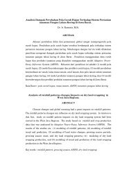
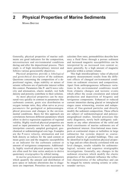
2.2 Porositiy and Wet Bulk DensityFig. 2.4 Comparison of wet bulk densities determined on discrete samples by weight and volume measurements andcalculated from gamma ray attenuation. (a) Cross plot of wet bulk densities of gravity cores PS1821-6 from theAntarctic and PS1725-2 from the Arctic Ocean. The dashed lines indicate a difference of ±5% between both data sets.(b) Wet bulk density logs derived from gamma ray attenuation for two 1 m long core sections of gravity core PS1725-2.Superimposed are density values measured on discrete samples. Modified after Gerland and Villinger (1995).33

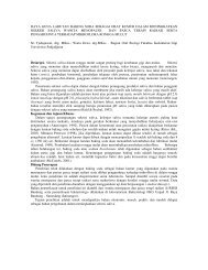
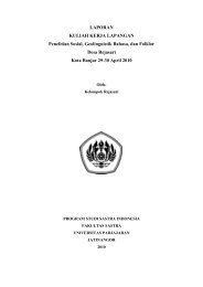
2Physical Properties of Marine Sedimentsconstant (a) and formation factor (F) togethercharacterize a specific environment. Table 2.1summarizes the values of (a) and (m) derived froma linear least square fit to the log-log display ofthe data sets and shortly describes the sedimentcompositions.With these values for (a) and (m) calibratedporosity logs are calculated which agree well withporosities determined on discrete samples (Fig.2.8, black curves). The error in porosity that mayresult from using the ‘standard’ Boyce’s (1968)values for (a) and (m) instead of those derivedfrom the calibration appears in two different ways(gray curves). (1) The amplitude of the downcoreporosity variations might be too large, as isillustrated by core GeoB2110-4 from the BrazilianContinental Margin. (2) The log might be shiftedto higher or lower porosities, as is shown by coreGeoB1517-1 from the Ceará Rise. Only if linearregression results in values for (a) and (m) closeto Boyce’s (1968) coefficients the error in theporosity log is negligible (core GeoB1701-4 fromthe Niger Mouth).In order to compute absolutely correct wet bulkdensities from calibrated porosity logs a graindensity must be assumed. For most terrigenous andcalcareous sediment cores this parameter is notvery critical as it often only changes by fewpercent downcore (e.g. 2.6 - 2.7 g cm -3 ). However, incores from the Antarctic Polar Frontal Zone wherean interlayering of diatomaceous and calcareousoozes indicates the advance and retreat of theoceanic front during glacial and interglacial stagesgrain densities may vary between about 2.0 and2.8 g cm -3 . Here, depth-dependent values musteither be known or modeled in order to get correctwet bulk density variations from resistivitymeasurements. An example for this approach areresistivity measurements on ODP core 690C fromthe Maud Rise (Fig. 2.9). While the carbonate log(b) clearly indicates calcareous layers with highand diatomaceous layers with zero CaCO 3percentages (O’Connell 1990), the resistivitybasedporosity log (a) only scarcely reflects theselithological changes. The reason is thatcalcareous and diatomaceous oozes are characterizedby high inter- and intraporosities incorporatedin and between hollow foraminifera and diatomshells. In contrast, the wet bulk density logmeasured onboard of JOIDES Resolution by gammaray attenuation ((c), gray curve) reveals pronouncedvariations. They obviously correlate with the CaCO 3-content and can thus only be attributed to downcorechanges in the grain density. So, a grain densitymodel (d) was developed. It averages the densitiesof carbonate (ρ carb= 2.8 g cm -3 ) and biogenic opal(ρ opal= 2.0 g cm -3 ) (Barker, Kennnett et al. 1990)according to the fractional CaCO 3-content (C),ρ model= C×ρ carb+ (1 - C)×ρ opal. Based on this modelwet bulk densities ((c), black curve) were derived fromTable 2.1 Geographical coordinates, water depth, core length, region and composition of the sediment coresconsidered in Figure 2.7. The cementation exponent (m) and the constant (a) are derived from the slope andintercept of a linear least square fit to the log-log display of formation factors versus porosities.Core Coordinates Water Core Region Sediment Factor CementationDepth Length Composition (a) Exponent (m)GeoB 35°12.4'S 4058 m 6.97 m Hunter foram.-nannofossil 1,6 1,31306-2 26°45.8'W Gap ooze, sandyGeoB 04°44.2'N 4001 m 6.89 m Ceará nannofossil-foram. 1,3 2,11517-1 43°02.8'W Rise oozeGeoB 01°57.0'N 4162 m 7.92 m Niger clayey mud, foram. 1,4 1,41701-4 03°33.1'E Mouth bearingGeoB 29°58.2'S 5084 m 7.45 m Cape red clay 1,0 2,81724-2 08°02.3'E BasinGeoB 28°38.8'S 3011 m 8.41 m Braz. Cont. pelagic clay. Foram. 0,8 3,32110-4 45°31.1'W Margin bearingGeoB 05°06.4'S 1830 m 14.18 m Congo hemipelagic mud, 0,8 5,32302-2 10°05.5'E Fan diatom bearing, H 2 S38

2.2 Porositiy and Wet Bulk Densitythe porosity log which agree well with the gammaray attenuation densities ((c), gray curve) andshow less scatter.Though resistivities are only measured halfautomaticallyincluding a manual insertion andremoval of the probe, increments of 1 - 2 cm canbe realized within an acceptable time so that morefine-scale structures can be resolved than byanalysis of discrete samples. However, the realadvantage compared to an automated gamma rayattenuation logging is that the resistivity measurementsystem can easily be transported, e.g.onboard of research vessels or to core repositories,while the transport of radioactive sourcesrequires special safety precautions.2.2.4 Electrical Resistivity(Inductive Method)A second, non-destructive technique to determineporosities by resistivity measurements uses a coilas sensor. A current flowing through the coilinduces an electric field in the unsplit sedimentcore while it is automatically transported throughFig. 2.8 Porosity logs determined by resistivity measurements on three gravity cores from the South Atlantic (seealso Fig. 2.7 and Table 2.1). Gray curve: Boyce’s (1968) values were used for the constants (a) and (m). Black curve:(a) and (m) were derived from the slope and intercept of a linear least square fit. These values are given at the topof each log. Superimposed are porosities determined on discrete samples by weight and volume measurements(unpublished data from P. Müller, University Bremen, Germany).39

2Physical Properties of Marine SedimentsFig. 2.9 Model based computation of a wet bulk density log from resistivity measurements on ODP core 690C. (a)Porosity log derived from formation factors having used Boyce’s (1968) values for (a) and (m) in Archie’s law. (b)Carbonate content (O’Conell 1990). (c) Wet bulk density log analyzed from gamma ray attenuation measurementsonboard of JOIDES Resolution (gray curve). Superimposed is the wet bulk density log computed from electricalresistivity measurements on archive halves of the core (black curve) having used the grain density model shown in(d). Unpublished data from B. Laser and V. Spieß, University Bremen, Germany.40

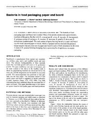
2.2 Porositiy and Wet Bulk Densitythe centre of the coil (Gerland et al. 1993). Thisinduced electric field contains information on themagnetic and electric properties of the sediment.Generally, the coil characteristic is defined bythe quality value(Q)L( ω)Q = ω ⋅(2.13)R ( ω)(L(ω)) is the inductance, (R(ω)) the resistance and(ω) the (angular) frequency of the alternatingcurrent flowing through the coil (Chelkowski1980). The inductance (L(ω)) depends on the numberof windings, the length and diameter of thecoil and the magnetic permeability of the coilmaterial. The resistance (R(ω)) is a superpositionof the resistance of the coil material and losses ofthe electric field induced in the core. It increaseswith decreasing resistivity in the sediment.Whether the inductance or the resistance is ofmajor importance depends on the frequency of thecurrent flowing through the coil. Changes in theinductance (L(ω)) can mainly be measured ifcurrents of some kilohertz frequency or less areused. They simultaneously indicate variations inthe magnetic susceptibility while the resistance(R(ω)) is insensitive to changes in the resistivityof the sediment. In contrast, operating withcurrents of several megahertz allows to measurethe resistivity of the sediment by changes of thecoil resistance (R(ω)) while variations in themagnetic susceptibility do not affect the inductance(L(ω)). The examples presented here weremeasured with a commercial system (Scintrex CTU 2)which produces an output voltage that is proportionalto the quality value (Q) of the coil at afrequency of 2.5 MHz, and after calibration isinversely proportional to the resistivity of thesediment.The induced electric field is not confined tothe coil position but extends over some sedimentvolume. Hence, measurements of the resistance(R(ω)) integrate over the resistivity distribution onboth sides of the coil and provide a smoothed,low-pass filtered resistivity record. The amount ofsediment volume affected by the inductionprocess increases with larger coil diameters. Theshape of the smoothing function can be measuredfrom the impulse response of a thin metal plateglued in an empty plastic core liner. For a coil ofabout 14 cm diameter this gaussian-shapedfunction has a half-width of 4 cm (Fig. 2.10), sothat the effect of an infinitely small resistivityanomaly is smeared over a depth range of 10 - 15 cm.This smoothing effect is equivalent to convolutionof a source wavelet with a reflectivity functionin seismic applications and can accordinglybe removed by deconvolution algorithms. However,only few applications from longcore paleomagneticstudies are known up to now (Constableand Parker 1991; Weeks et al. 1993).Fig. 2.10 Impulse response function of a thin metal plate measured by the inductive method with a coil of about 14 cmdiameter. Modified after Gerland et al. (1993).41

2Physical Properties of Marine SedimentsThe low-pass filtering effect particularly becomesobvious if resistivity logs measured by the galvanicand inductive method are compared. Figure 2.11displays such an example for a terrigenous corefrom the Weddell Sea (PS1635-1) and a biogenicforaminiferal and diatomaceous core from theMaud Rise (PS1836-3) in the Antarctic Ocean.Resistivities differ by maximum 15% (Fig. 2.11a), arather high value which mainly results from corePS1635-1. Here, the downcore logs illustrate thatthe inductive methods produces lower resistivitiesthan the galvanic method (Fig. 2.11b). In detail,the galvanic resistivity log reveals a lot of pronounced,fine-scale variations which cannot beresolved by induction measurements but aresmeared along the core depth. For the biogeniccore PS1836-3 this smoothing is not so importantbecause lithology changes more gradually.2.3 PermeabilityPermeability describes how easy a fluid flowsthrough a porous medium. Physically it is definedby Darcy’s lawκ ∂pq = ⋅(2.14)η ∂xwhich relates the flow rate (q) to the permeability(κ) of the pore space, the viscosity (η) of the porefluid and the pressure gradient ( ∂p/ ∂x) causingthe fluid flow. Simultaneously, permeabilitydepends on the porosity (φ) and grain size distributionof the sediment, approximated by the meangrain size (d m). Assuming that fluid flow can besimulated by an idealized flow through a bunch ofcapillaries with uniform radius (d m/2) (HagenPoiseuille’s flow) permeabilities can for instancebe estimated from Kozeny-Carman’s equation(Carman 1956; Schopper 1982)23φκ =d m ⋅(2.15)36kφ( 1−) 2This relation is approximately valid for unconsolidatedsediments of 30 - 80% porosity (Carman1956). It is used for both geotechnical applicationsto estimate permeabilities of soil (Lambe andWhitman 1969) and seismic modeling of wavepropagation in water-saturated sediments (Biot1956a, b; Hovem and Ingram 1979; Hovem 1980;Ogushwitz 1985). (κ) is a constant which dependson pore shape and tortuosity. In case of parallel,cylindrical capillaries it is about 2, for sphericalsediment particles about 5, and in case of highporosities ≥ 10 (Carman 1956).However, this is only one approach to estimatepermeabilities from porosities and mean grainsizes. Other empirical relations exist, particularlyfor regions with hydrocarbon exploration (e.g.Gulf of Mexico, Bryant et al. 1975) or fluid venting(e.g. Middle Valley, Fisher et al. 1994) whichcompute depth-dependent permeabilities fromporosity logs or take the grain size distributionand clay content into account.Direct measurements of permeabilities in unconsolidatedmarine sediments are difficult, andonly few examples are published. They confine tomeasurements on discrete samples with a speciallydeveloped tool (Lovell 1985), to indirect estimationsby resistivity measurements (Lovell 1985),and to consolidation tests on ODP cores using amodified medical tool (Olsen et al. 1985). Thesemeasurements are necessary to correct for theelastic rebound (MacKillop et al. 1995) and todetermine intrinsic permeabilities at the end ofeach consolidation step (Fisher et al. 1994). InSection 2.4.2 a numerical modeling and inversionscheme is described which estimates permeabilitiesfrom P-wave attenuation and dispersioncurves (c.f. also section 3.6).2.4 Acoustic and Elastic PropertiesAcoustic and elastic properties are directly concernedwith seismic wave propagation in marinesediments. They encompass P- and S-wave velocityand attenuation and elastic moduli of thesediment frame and wet sediment. The mostimportant parameter which controls size andresolution of sedimentary structures by seismicstudies is the frequency content of the sourcesignal. If the dominant frequency and bandwidthare high, fine-scale structures associated withpore space and grain size distribution affect theelastic wave propagation. This is subject of ultrasonictransmission measurements on sedimentcores (Sects. 2.4 and 2.5). At lower frequencieslarger scale features like interfaces with differentphysical properties above and below and bedformslike mud waves, erosion zones and channellevee systems are the dominant structures imaged42

2.4 Acoustic and Elastic PropertiesFig. 2.11 Comparison of electrical resistivities (galv.) measured with the small hand-held probe and determined bythe inductive method (ind.) for the gravity cores PS1635-1 and PS1836-3. (a) Cross plots of both data sets. Thedashed lines indicate a difference of 15%. (b) Downcore resistivity logs determined by both methods. Modified afterGerland et al. (1993).43

2Physical Properties of Marine Sedimentsby sediment echosounder and multi-channelseismic surveys (Sect. 2.6).In this section first Biot’s viscoelastic model issummarized which simulates high- and lowfrequencywave propagation in water-saturatedsediments by computing phase velocity andattenuation curves. Subsequently, analysistechniques are introduced which derive P-wavevelocities and attenuation coefficients fromultrasonic signals transmitted radially acrosssediment cores. Additional physical properties likeS-wave velocity, elastic moduli and permeabilityare estimated by an inversion scheme.2.4.1 Biot-Stoll ModelTo describe wave propagation in marine sedimentsmathematically, various simple to complex modelshave been developed which approximate thesediment by a dilute suspension (Wood 1946) oran elastic, water-saturated frame (Gassmann 1951;Biot 1956a, b). The most common model whichconsiders the microstructure of the sediment andsimulates frequency-dependent wave propagationis based on Biot’s theory (Biot 1956a, b). It includesWood’s suspension and Gassmann’s elastic framemodel as low-frequency approximations andcombines acoustic and elastic parameters - P- andS-wave velocity and attenuation and elastic moduli- with physical and sedimentological parameterslike mean grain size, porosity, density and permeability.Based on Biot’s fundamental work Stoll (e.g.1974, 1977, 1989) reformulated the mathematicalbackground of this theory with a simplifieduniform nomenclature. Here, only the main physicalprinciples and equations are summarized. For adetailed description please refer to one of Stoll’spublications or Biot’s original papers.The theory starts with a description of themicrostructure by 11 parameters. The sedimentgrains are characterized by their grain density (ρ g)and bulk modulus (K g), the pore fluid by itsdensity (ρ f), bulk modulus (K f) and viscosity (η).The porosity (φ) quantifies the amount of porespace. Its shape and distribution are specified bythe permeability (κ), a pore size parametera=d m/3⋅φ/(1-φ), d m= mean grain size (Hovem andIngram 1979; Courtney and Mayer 1993), andstructure factor a’=1-r 0(1-φ -1 ) (0 ≤ r 0≤ 1) indicatinga tortuosity of the pore space (Berryman 1980).The elasticity of the sediment frame is consideredby its bulk and shear modulus (K mand µ m).An elastic wave propagating in water-saturatedsediments causes different displacements ofthe pore fluid and sediment frame due to theirdifferent elastic properties. As a result (global)fluid motion relative to the frame occurs and canapproximately be described as Poiseuille’s flow.The flow rate follows Darcy’s law and depends onthe permeability and viscosity of the pore fluid.Viscous losses due to an interstitial pore waterflow are the dominant damping mechanism. Intergranularfriction or local fluid flow can additionallybe included but are of minor importance inthe frequency range considered here.Based on generalized Hooke’s law andNewton’s 2. Axiom two equations of motions arenecessary to quantify the different displacementsof the sediment frame and pore fluid. For P-wavesthey are (Stoll 1989)∇2∇22∂( H ⋅e− C ⋅ζ) = ( ρ ⋅e− ρ ⋅ζ)∂ t2∂( C ⋅e− M ⋅ζ) = ( ρ ⋅e− m ⋅ζ)∂ t22ff(2.16a)η ∂ζ− ⋅κ ∂ t(2.16b)Similar equations for S-waves are given byStoll (1989). Equation 2.16a describes the motionof the sediment frame and Equation 2.16b the motionof the pore fluid relative to the frame.ande = div (u)(2.16c) ζ =φ ⋅ div ( u − U )(2.16d)are the dilatations of the frame and between porefluid and frame ( u = displacement of the frame,U = displacement of the pore fluid). The term( η κ ⋅ ∂ζ ∂ t ) specifies the viscous losses due toglobal pore fluid flow, and the ratio ( η κ ) the viscousflow resistance.The coefficients (H), (C), and (M) define the elasticproperties of the water-saturated model. They areassociated with the bulk and shear moduli of thesediment grains, pore fluid and sediment frame (Κ g ),(Κ f ), (Κ m ), (µ m ) and with the porosity (φ) byΗ = (Κ g - K m ) 2 / (D - K m ) + K m + 4 / 3 · µ m(2.17a)C = (K g · (K g - K m )) / (D - K m ) (2.17b)44

2.4 Acoustic and Elastic PropertiesΜ = Κ g2/ (D - K m )D = K g · (1 + φ · ( K g /K f - 1))(2.17c)(2.17d)The apparent mass factor m = a’⋅ρ f /φ (a’ ≥ 1) inEquation 2.16b considers that not all of the porefluid moves along the maximum pressure gradientin case of tortuous, curvilinear capillaries. As a resultthe pore fluid seems to be more dense, withhigher inertia. (a’) is called structure factor and isequal to 1 in case of uniform parallel capillaries.In the low frequency limit H - 4/3µ m(Eq. 2.17a)represents the bulk modulus computed by Gassmann(1951) for a ‘closed system’ with no porefluid flow. If the shear modulus (µ m) of the frame isadditionally zero, the sediment is approximated bya dilute suspension and Equation 2.17a reduces tothe reciprocal bulk modulus of Wood’s equation for‘zero’ acoustic frequency, (K -1 = φ/K f+ (1-φ)/K g;Wood 1946).Additionally, Biot (1956a, b) introduced acomplex correction function (F) which accountsfor a frequency-dependent viscous flow resistance(η/κ). In fact, while the assumption of anideal Poiseuille flow is valid for lower frequencies,deviations of this law occur at higher frequencies.For short wavelengths the influence of pore fluidviscosity confines to a thin skin depth close tothe sediment frame, so that the pore fluid seems tobe less viscous. To take these effects into accountthe complex function (F) modifies the viscous flowresistance (η/κ) as a function of pore size, porefluid density, viscosity and frequency. A completedefinition of (F) can be found in Stoll (1989).The equations of motions 2.16 are solved by aplane wave approach which leads to a 2 x 2determinant for P-waves⎛det⎜H ⋅k⎜⎝C ⋅ k222− ρω2− ρ ωf22mω− M ⋅k22ρ ω − C ⋅ kf⎞⎟ = 0− iωFηκ⎟⎠(2.18)and a similar determinant for S-waves (Stoll 1989).The variable k(ω) = k r(ω) + ik i(ω) is the complexwavenumber. Computations of the complex zeroesof the determinant result in the phase velocityc(ω) = ω/k r(ω) and attenuation coefficient α(ω) =k i(ω) as real and imaginary parts. Generally, thedeterminant for P-waves has two and that for S-waves one zero representing two P- and one S-wave propagating in the porous medium. The firstP-wave (P-wave of first kind) and the S-wave arewell known from conventional seismic wavepropagation in homogeneous, isotropic media.The second P-wave (P-wave of second kind) issimilar to a diffusion wave which is exponentiallyattenuated and can only be detected by speciallyarranged experiments (Plona 1980).An example of such frequency-dependent phasevelocity and attenuation curves presents Figure 2.12for P- and S-waves together with the slope (power (n))of the attenuation curves (α = k ⋅ f n ). Three sets ofphysical properties representing typical sand, siltand clay (Table 2.2) were used as model parameters.The attenuation coefficients show a significantchange in their frequency dependence.They follow an α∼f 2 power law for low and anα∼√f law for high frequencies and indicate acontinuously decreasing power (n) (from 2 to 0.5)near a characteristic frequency f c= (ηφ)/(2πκρ f).This characteristic frequency depends on themicrostructure (porosity (φ), permeability (κ)) andpore fluid (viscosity (η), density (ρ f)) of the sedimentand is shifted to higher frequencies ifporosity increases and permeability decreases.Below the characteristic frequency the sedimentframe and pore fluid moves in phase and couplingbetween solid and fluid components is at maximum.This behaviour is typical for clayey sedimentsin which low permeability and viscousfriction prevent any relative movement betweenpore fluid and frame up to several MHz, in spite oftheir high porosity. With increasing permeabilityand decreasing porosity the characteristicfrequency diminishes so that in sandy sedimentsmovements in phase only occur up to about 1 kHz.Above the characteristic frequency wavelengthsare short enough to cause relative motionsbetween pore fluid and frame.Phase velocities are characterized by a lowandhigh-frequency plateau with constant valuesand a continuous velocity increase near the characteristicfrequency. This dispersion is difficult todetect because it is confined to a small frequencyband. Here, dispersion could only be detectedfrom 1 - 10 kHz in sand, from 50 - 500 kHz in siltand above 100 MHz in clay. Generally, velocities incoarse-grained sands are higher than in finegrainedclays.S-waves principally exhibit the same attenuationand velocity characteristics as P-waves.However, at the same frequency attenuation is45

2Physical Properties of Marine SedimentsFig. 2.12 Frequency-dependent attenuation and phase velocity curves and power (n) of the attenuation law α = k ⋅ f ncomputed for P-and S-waves in typical sand, silt and clay. The gray-shaded areas indicate frequency bands typical forultrasonic measurements on sediment cores (50 - 500 kHz) and sediment echosounder surveys (0.5 - 10 kHz). Modifiedafter Breitzke (1997).46

2.4 Acoustic and Elastic Propertiesabout one magnitude higher, and velocities aresignificantly lower than for P-waves. The consequenceis that S-waves are very difficult to recorddue to their high attenuation, though they are ofgreat value for identifying fine-scale variations inthe elasticity and microstructure of marine sediments.This is even valid if the low S-wave velocitiesare taken into account and lower frequenciesare used for S-wave measurements than for P-wave recordings.The two gray-shaded areas in Figure 2.12 marktwo frequency bands typical for ultrasonic studieson sediment cores (50 - 500 kHz) and sedimentechosounder surveys (0.5 - 10 kHz). They aredisplayed in order to point to one characteristic ofacoustic measurements. Attenuation coefficientsanalyzed from ultrasonic measurements on sedimentcores cannot directly be transferred tosediment echosounder or seismic surveys. Primarilythey only reflect the microstructure of thesediment. Rough estimates of the attenuation inseismic recordings from ultrasonic core measurementscan be derived if ultrasonic attenuation ismodeled, and attenuation coefficients are extrapolatedto lower frequencies by such model curves.2.4.2 Full Waveform Ultrasonic CoreLoggingTo measure the P-wave velocity and attenuationillustrated by Biot-Stoll’s model an automated, PCcontrolledlogging system was developed whichrecords and stores digital ultrasonic P-waveformstransmitted radially across marine sediment cores(Breitzke and Spieß 1993). These transmissionmeasurements can be done at arbitrary small depthTable 2.2 Physical properties of sediment grains, pore fluid and sediment frame used for the computation ofattenuation and phase velocity curves according to Biot-Stoll’s sediment model (Fig. 2.12).Parameter Sand Silt ClaySediment GrainsBulk Modulus Κ g [10 9 Pa] 38 38 38Density ρ g [g cm -3 ] 2.67 2.67 2.67Pore FluidBulk Modulus Κ f [10 9 Pa] 2.37 2.37 2.37Density ρ f [g cm -3 ] 1.024 1.024 1.024Viscosity η [10 -3 Pa⋅s] 1.07 1.07 1.07Sediment FrameBulk Modulus Κ m [10 6 Pa] 400 150 20Shear Modulus µ m [10 6 Pa] 240 90 12Poisson Ratio σ m0.25 0.25 0.25Pore SpacePorosity φ [%] 50 60 80Mean Grain Size d m [10 -6 m] 70 30 2Permeability κ [m 2 ] 5.4·10 -11 2.3·10 -12 7.1·10 -15Pore Size Parameter a = d m /3φ /(1-φ ) [10 -6 m] 23 15 2.7Ratio κ / a 2 0.1 0.01 0.001Structure Factor a' = 1-r 0 (1-φ -1 ) 1.5 1.3 1.1Constant r 00.5 0.5 0.547

2Physical Properties of Marine SedimentsFig. 2.13 Full waveform ultrasonic core logging, from lithology controlled single traces to the gray shaded pixel graphic of transmission seismograms, and P-wavevelocity and attenuation logs derived from the transmission data. The single traces on the left-hand side reflect true amplitudes while the wiggle traces of the coresegment and the pixel graphic are normalized to maximum values. Data from Breitzke et al. (1996).48

2.4 Acoustic and Elastic Propertiesincrements so that the resulting seismogram sectionscan be combined to an ultrasonic image of thecore.Figure 2.13 displays the most prominent effectsinvolved in full waveform ultrasonic core logging.Gravity core GeoB1510-2 from the westernequatorial South Atlantic serves as an example. Thelithology controlled single traces and amplitudespectra demonstrate the influence of increasinggrain sizes on attenuation and frequency contentof transmission seismograms. Compared to areference signal in distilled water, the signal shaperemains almost unchanged in case of wavepropagation in fine-grained clayey sediments (1stattenuated trace). With an increasing amount ofsilty and sandy particles the signal amplitudes arereduced due to an enhanced attenuation of highfrequencycomponents (2nd and 3rd attenuatedtrace). This attenuation is accompanied by achange in signal shape, an effect which isparticularly obvious in the normalized wiggle tracedisplay of the 1 m long core segment. While theupper part of this segment is composed of finegrainednannofossil ooze, a calcareous foraminiferalturbidite occurs in the lower part. The downwardcoarsening of the graded bedding causessuccessively lower-frequency signals which caneasily be distinguished from the high-frequencytransmission seismograms in the upper fine-grainedpart. Additionally, first arrival times are lower in thecoarse-grained turbidite than in fine-grainednannofossil oozes indicating higher velocities insilty and sandy sediments than in the clayey part.A conversion of the normalized wiggle traces to agray-shaded pixel graphic allows us to present thefull transmission seismogram information on ahandy scale. In this ultrasonic image of thesediment core lithological changes appear assmooth or sharp phase discontinuities resultingfrom the low-frequency waveforms in silty andsandy layers. Some of these layers indicate agraded bedding by downward prograding phases(1.60 - 2.10 m, 4.70 - 4.80 m, 7.50 - 7.60 m). The P-wave velocity and attenuation log analyzed fromthe transmission seismograms support theinterpretation. Coarse-grained sandy layers arecharacterized by high P-wave velocities and attenuationcoefficients while fine-grained parts reveallow values in both parameters. Especially, attenuationcoefficients reflect lithological changesmuch more sensitively than P-wave velocities.While P-wave velocities are determined onlineduring core logging using a cross-correlationtechnique for the first arrival detection (Breitzkeand Spieß 1993)vPd outside − 2dliner= (2.19)t − 2tliner(d outside= outer core diameter, 2 d liner= doubleliner wall thickness, t = detected first arrival,2t liner= travel time across both liner walls),attenuation coefficients are analyzed by a postprocessingroutine. Several notches in the amplitudespectra of the transmission seismogramscaused by the resonance characteristics of theultrasonic transducers required a modification ofstandard attenuation analysis techniques (e.g.Jannsen et al. 1985; Tonn 1989, 1991). Here, amodification of the spectral ratio method isapplied (Breitzke et al. 1996). It defines a windowof bandwidth (b i= f ui- f li) in which the spectralamplitudes are summed (Fig. 2.14a).∑( f x) A( f x)mifA , , (2.20)= ui fi= fliThe resulting value ( Af (mi, x)) is related tothat part of the frequency band which predominantlycontributes to the spectral sum, i.e. to thearithmetic mean frequency (f mi) of the spectralamplitude distribution within the i th band. Subsequently,for a continuously moving window aseries of attenuation coefficients (α(f mi)) is computedfrom the natural logarithm of the spectralratio of the attenuated and reference signal( f )⎡⎢⎣A( f mi , x)( f , x)⎤⎥⎦nα mi = lnx = k ⋅ f (2.21)⎢ Arefmi⎥Plotted in a log α - log f diagram the power (n)and logarithmic attenuation factor (log k) can bedetermined from the slope and intercept of a linearleast square fit to the series of (f mi,α(f mi)) pairs(Fig. 2.14b). Finally, a smoothed attenuationcoefficient α(f) = k ⋅ f n is calculated for thefrequency (f) using these values for (k) and (n).Figure 2.14b shows several attenuation curves(α(f mi)) analyzed along the turbidite layer of coreGeoB1510-2. With downward-coarsening grainsizes attenuation coefficients increase. Each linearregression to one of these curves provide a power(n) and attenuation factor (k), and thus one valueα = k ⋅ f n on the attenuation log of the completecore (Fig. 2.14c).i49

2Physical Properties of Marine SedimentsFig. 2.14 Attenuation analysis by the smoothed spectral ratio method. (a) Definition of a moving window ofbandwidth b i=f ui-f li, in which the spectral amplitudes are summed. (b) Seven attenuation curves analyzed from theturbidite layer of gravity core GeoB1510-2 and linear regression to the attenuation curve in 1.82 m depth. (c)Attenuation log of gravity core GeoB1510-2 for 400 kHz frequency. Data from Breitzke et al. (1996).50

2.4 Acoustic and Elastic PropertiesAs the P-wave attenuation coefficientobviously depends on the grain size distributionof the sediment it can be used as a proxy parameterfor the mean grain size, i.e. for a sedimentologicalparameter which is usually onlymeasured at coarse increments due to the timeconsuminggrain size analysis methods. Forinstance, this can be of major importance incurrent controlled sedimentation environmentswhere high-resolution grain size logs mightindicate reduced or enhanced current intensities.If the attenuation coefficients and mean grainsizes analyzed on discrete samples of coreGeoB1510-2 are displayed as a cross plot a secondorder polynomial can be derived from a leastsquare fit (Fig. 2.15a). This regression curve thenallows to predict mean grain sizes using theattenuation coefficient as proxy parameter. Theaccuracy of the predicted mean grain sizes illustratesthe core log in Figure 2.15b. The predictedgray shaded log agrees well with the superimposeddots of the measured data.Similarly, P-wave velocities can also be used asproxy parameters for a mean grain size prediction.However, as they cover only a small range (1450 -1650 m/s) compared to attenuation coefficients (20- 800 dB/m) they reflect grain size variations lesssensitively.Generally, it should be kept in mind, that theregression curve in Figure 2.15 is only an example.Its applicability is restricted to that range ofattenuation coefficients for which the regressioncurve was determined and to similar sedimentationenvironments (calcareous foraminiferal andnannofossil ooze). For other sediment compositionsnew regression curves must be determined,which are again only valid for that specificsedimentological setting.Fig. 2.15 (a) Attenuation coefficients (at 400 kHz) of gravity core GeoB1510-2 versus mean grain sizes. The solidline indicates a second degree polynomial used to predict mean grain sizes from attenuation coefficients. (b)Comparison of the predicted mean grain size log (gray shaded) with the data measured on discrete samples (soliddots). Mean grain sizes are given in Φ = -log 2d, d = grain diameter in mm. Modified after Breitzke et al. (1996).51

2Physical Properties of Marine SedimentsBiot-Stoll’s theory allows us to model P-wavevelocities and attenuation coefficients analyzed fromtransmission seismograms. As an example Figure 2.16displays six data sets for the turbidite layer of coreGeoB1510-2. While attenuation coefficients wereanalyzed as described above frequency dependent P-wave velocities were determined from successivebandpass filtered transmission seismograms (Courtneyand Mayer 1993; Breitzke 1997). Porosities andmean grain sizes enter the modeling computations viathe pore size parameter (a) and structure factor (a’).Physical properties of the pore fluid and sedimentgrains are the same as given in Table 2.2. A bulk andshear modulus of 10 and 6 MPa account for theelasticity of the frame. As the permeability is theparameter which is usually unknown but has thestrongest influence on attenuation and velocitydispersion, model curves were computed for threeconstant ratios κ/a 2 = 0.030, 0.010 and 0.003 ofpermeability (κ) and pore size parameter (a). Theresulting permeabilities are given in each diagram.These theoretical curves show that the attenuationand velocity data between 170 and 182 cm depth canconsistently be modeled by an appropriate set ofinput parameters. Viscous losses due to a global porewater flow through the sediment are sufficient to explainthe attenuation in these sediments. Only if theturbidite base is approached (188 - 210 cm depth) theattenuation and velocity dispersion data successivelydeviate from the model curves probably dueto an increasing amount of coarse-grained foraminifera.An additional damping mechanism whichmight either be scattering or resonance within thehollow foraminifera must be considered.Based on this modeling computations aninversion scheme was developed which automaticallyiterates the permeability and minimizesthe difference between measured and modeledattenuation and velocity data in a least squaresense (Courtney and Mayer 1993; Breitzke 1997).As a result S-wave velocities and attenuationcoefficients, permeabilities and elastic moduli ofwater-saturated sediments can be estimated. Theyare strictly only valid if attenuation and velocitydispersion can be explained by viscous losses. Incoarse-grained parts deviations must be takeninto account for the estimated parameters, too.Applied to the data of core GeoB1510-2 in 170, 176and 182 cm depth S-wave velocities of 67, 68 and74 m/s and permeabilities of 5·10 -13 , 1·10 -12 and3·10 -12 m 2 result from this inversion scheme.2.5 Sediment ClassificationFull waveform ultrasonic core logging was appliedto terrigenous and biogenic sediment cores toanalyze P-wave velocities and attenuation coefficientstypical for the different settings. Togetherwith the bulk parameters and the physical propertiesestimated by the inversion scheme they formthe data base for a sediment classification whichidentifies different sediment types from theirTable 2.3 Geographical coordinates, water depth, core length, region and composition of the sediment coresconsidered for the sediment classification in Section 2.5.Core Coordinates Water Core Region SedimentDepth Length Composition40KL 07°33.1'N 3814 m 8.46 m Bengal terrigenous clay, silt, sand85°29.7'EFan47KL 11°10.9'N 3293 m 10.00 m Bengal terrigenous clay, silt, sand;88°24.9'E Fan foram. and nannofossil oozeGeoB 30°27.1'S 3941 m 8.19 m Rio Grande foram. and nannofossil ooze2821-1 38°48.9'W RisePS 46°56.1'S 4102 m 17.65 m Meteor diatomaceous mud/ooze; few2567-2 06°15.4'E Rise foram. and nannofossil layers52

2.5 Sediment ClassificationFig. 2.16 Comparison of P-wave attenuation and velocity dispersion data derived from ultrasonic transmission seismogramswith theoretical curves based on Biot-Stoll’s model for six traces of the turbidite layer of gravity core GeoB1510-2.Permeabilities vary in the model curves according to constant ratios κ/a 2 = 0.030, 0.010, 0.003 (κ = permeability, a = pore sizeparameter). The resulting permeabilities are given in each diagram. Modified after Breitzke et al. (1996).53

2Physical Properties of Marine Sedimentsacoustic and elastic properties. Table 2.3 summarizesthe cores used for this sediment classification.2.5.1 Full Waveform Core Logs asAcoustic ImagesThat terrigenous, calcareous and biogenic siliceoussediments differ distinctly in their acousticproperties is shown by four transmission seismogramsections in Figure 2.17. Terrigenoussediments from the Bengal Fan (40KL, 47KL) arecomposed of upward-fining sequences of turbiditescharacterized by upward decreasing attenuationsand P-wave velocities. Coarse-grainedbasal sandy layers can easily be located by lowfrequencywaveforms and high P-wave velocities.Calcareous sediments from the Rio Grande Rise(GeoB2821-1) in the western South Atlantic alsoexhibit high- and low-frequency signals whichscarcely differ in their P-wave velocities. In thesesediments high-frequency signals indicate finegrainednannofossil ooze while low-frequencysignals image coarse-grained foraminiferal ooze.The sediment core from the Meteor Rise(PS2567-2) in the Antarctic Ocean is composed ofdiatomaceous and foraminiferal-nannofossil oozedeposited during an advance and retreat of thePolar Frontal Zone in glacial and interglacialstages. Opal-rich, diatomaceous ooze can be identifiedfrom high-frequency signals while foraminiferal-nannofossilooze causes higher attenuationand low-frequency signals. P-wave velocitiesagain only show smooth variations.Acoustic images of the complete core lithologiespresent the colour-encoded graphics of thetransmission seismograms, in comparison to thelithology derived from visual core inspection (Fig.2.18). Instead of normalized transmission seismogramsinstantaneous frequencies are displayedhere (Taner et al. 1979). They reflect the dominantfrequency of each transmission seismogram astime-dependent amplitude, and thus directlyindicate the attenuation. Highly attenuated lowfrequencyseismograms appear as warm red towhite colours while parts with low attenuation andhigh-frequency seismograms are represented bycool green to black colours.In these attenuation images the sandy turbiditebases in the terrigenous cores from theBengal Fan (40KL, 47KL) can easily be distinguished.Graded beddings can also be identifiedfrom slightly prograding phases and continuouslydecreasing travel times. In contrast, the transitionto calcareous, pelagic sediments in the upper part(> 5.6 m) of core 47KL is rather difficult to detect.Only above 3.2 m depth a slightly increasedattenuation can be observed by slightly warmercolours at higher transmission times (> 140 µs). Inthis part of the core (> 3.2 m) sediments are mainlycomposed of coarse-grained foraminiferal ooze,while farther downcore (3.2 - 5.6 m) fine-grainednannofossils prevail in the pelagic sediments.The acoustic image of the calcareous core fromthe Rio Grande Rise (GeoB2821-1) shows muchmore lithological changes than the visual coredescription. Cool colours between 1.5 - 2.5 mdepth indicate unusually fine grain sizes (Breitzke1997). Alternately yellow/red and blue/blackcolours in the lower part of the core (> 6.0 m)reflect an interlayering of fine-grained nannofossiland coarse-grained foraminiferal ooze. Dating byorbital tuning shows that this interlayering coincideswith the 41 ky cycle of obliquity (vonDobeneck and Schmieder 1999) so that finegrainedoozes dominate during glacial and coarsegrainedoozes during interglacial stages.The opal-rich diatomaceous sediments in corePS2567-2 from the Meteor Rise are characterizedby a very low attenuation. Only 2 - 3 calcareouslayers with significantly higher attenuation(yellow and red colours) can be identified asprominent lithological changes.2.5.2 P- and S-Wave Velocity,Attenuation, Elastic Moduli andPermeabilityAs the acoustic properties of water-saturatedsediments are strongly controlled by the amountand distribution of pore space, cross plots of P-wave velocity and attenuation coefficient versusporosity clearly indicate the different bulk andelastic properties of terrigenous and biogenicsediments and can thus be used for an acousticclassification of the lithology. Additional S-wavevelocities (and attenuation coefficients) andelastic moduli estimated by least-square inversionspecify the amount of bulk and shear moduliwhich contribute to the P-wave velocity (Breitzke2000).The cross plots of the P-wave parameters ofthe four cores considered above illustrate thatterrigenous, calcareous and diatomaceoussediments can uniquely be identified from theirposition in both diagrams (Fig. 2.19). In terri-54

2.5 Sediment ClassificationFig. 2.17 Normalized transmission seismogram sections of four 1 m long core segments from different terrigenous and biogenic sedimentation environments.Seismograms were recorded with 1 cm spacing. Core depths are 5.49-6.43 m (40KL), 6.03-6.97 m (47KL), 5.26-6.14 m (GeoB2821-1), 12.77-13.60 m (PS2567-2).Maximum amplitudes of the transmission seismograms are plotted next to each section from 0 to ... mV, as given at the top.55

2Physical Properties of Marine SedimentsFig. 2.18 Ultrasonic images of the transmission measurements on cores 40KL, 47KL, GeoB2821-1 and PS2567-2 retrieved from different terrigenous and biogenicsedimentation environments. Displayed are the colour-encoded instantaneous frequencies of the transmission seismograms and the lithology derived from visual coreinspections.56

2.6 Sediment Echosoundinggenous sediments (40KL, 47KL) P-wave velocitiesand attenuation coefficients increase with decreasingporosities. Computed S-wave velocities arevery low (≈ 60 - 65 m s -1 ) and almost independentof porosity (Fig. 2.20a) whereas computed S-waveattenuation coefficients (at 400 kHz) vary stronglyfrom 4·10 3 dB m -1 in fine-grained sediments to1.5·10 4 dB m -1 in coarse-grained sediments (Fig.2.20b). Accordingly, shear moduli are also low anddo not vary very much (Fig. 2.21b) so that higherP-wave velocities in terrigenous sediments mainlyresult from higher bulk moduli (Fig. 2.21a).If calcareous, particularly foraminiferal components(FNO) are added to terrigenous sedimentsporosities become higher (≈ 70 - 80%, 47KL). P-wave velocities slightly increase from their minimumof 1475 m s -1 at 70% porosity to 1490 m s -1 at80% porosity (Fig. 2.19a) mainly due to an increasein the shear moduli from about 6.5 to 8.5 MPawhereas bulk moduli remain almost constant atabout 3000 MPa (Fig. 2.21b). However, a muchmore pronounced increase can be observed in theP-wave attenuation coefficients (Fig. 2.19b). Forporosities of about 80% they reach the samevalues (about 200 dB m -1 ) as terrigenous sedimentsof about 55% porosity, but can easily bedistinguished because of higher P-wave velocitiesin terrigenous sediments. S-wave attenuationcoefficients increase as well in these hemipelagicsediments from about 1·10 5 dB m -1 at 65% porosityto about 2.5·10 5 dB m -1 at 80% porosity (Fig.2.20b), and are thus even higher than interrigenous sediments.Calcareous foraminiferal and nannofossil oozes(NFO) show similar trends in both P-wave and S-wave parameters as terrigenous sediments, but areshifted to higher porosities due to their additionalintraporosities (GeoB2821-1; Figs. 2.19, 2.20).In diatomaceous oozes P- and S-wave wavevelocities increase again though porosities arevery high (>80%, PS2567-2; Figs. 2.19, 2.20). Here,the diatom shells build a very stiff frame whichcauses high shear moduli and S-wave velocities(Fig. 2.21). It is this increase in the shear moduliwhich only accounts for the higher P-wavevelocities while the bulk moduli remain almostconstant and are close to the bulk modulus of seawater (Fig. 2.21). P-wave attenuation coefficientsare very low in these high-porosity sediments(Fig. 2.19b) whereas S-wave attenuation coefficientsare highest (Fig. 2.20b).Permeabilities estimated from the least squareinversion mainly reflect the attenuation characteristicsof the different sediment types (Fig. 2.22).They reach lowest values of about 5·10 -14 m 2 infine-grained clayey mud and nannofossil ooze.Highest values of about 5·10 -11 m 2 occur in diatomaceousooze due to their high porosities.Nevertheless, it should be kept in mind that thesepermeabilities are only estimates based on theinput parameters and assumptions incorporated inBiot-Stoll’s model. For instance one of theseassumptions is that only mean grain sizes areused, but the influence of grain size distributionsis neglected. Additionally, the total porosity isusually used as input parameter for the inversionscheme without differentiation between inter- andintraporosities. Comparisons of these estimatedpermeabilities with direct measurements unfortunatelydo not exist up to know.2.6 Sediment EchosoundingWhile ultrasonic measurements are used to studythe structure and composition of sediment cores,sediment echosounders are hull-mounted acousticsystems which image the upper 10-200 m of sedimentcoverage by remote sensing surveys. They operatewith frequencies around 3.5-4.0 kHz. The examplespresented here were digitally recorded with thenarrow-beam Parasound echosounder andParaDIGMA recording system (Spieß 1993).2.6.1 Synthetic SeismogramsFigure 2.23 displays a Parasound seismogramsection recorded across an inactive channel of theBengal Fan. The sediments of the terrace weresampled by a 10 m long piston core (47KL). Itsacoustic and bulk properties can either be directlycompared to the echosounder recordings or bycomputations of synthetic seismograms. Suchmodeling requires P-wave velocity and wet bulkdensity logs as input parameters. From theproduct of both parameters acoustic impedances I= v P·ρ are calculated. Changes in the acousticimpedance cause reflections of the normallyincident acoustic waves. The amplitude of suchreflections is determined by the normal incidencereflection coefficient R = (I 2-I 1) / (I 2+I 1), with (I 1)and (I 2) being the impedances above and belowthe interface. From the series of reflectioncoefficients the reflectivity can be computed asimpulse response function, including all internal57

2Physical Properties of Marine SedimentsFig. 2.19 (a) P-wave velocities and (b) attenuation coefficients (at 400 kHz) versus porosities for the foursediment cores 40KL, 47KL, GeoB2821-1, and PS2567-2. NFO is nannofossil foraminiferal ooze, FNO isforaminiferal nannofossil ooze (nomenclature after Mazullo et al. (1988)). Modified after Breitzke (2000).58

2.6 Sediment EchosoundingFig. 2.20 (a) S-wave velocities and (b) attenuation coefficients (at 400 kHz) derived from least square inversionbased on Biot-Stoll’s theory versus porosities for the four sediment cores 40KL, 47KL, GeoB2821-1, and PS2567-2.NFO and FNO as in Figure 2.19. Modified after Breitzke (2000).59

2Physical Properties of Marine SedimentsFig. 2.21 (a) S-wave velocity versus P-wave velocity and (b) shear modulus versus bulk modulus derived from leastsquare inversion based on Biot-Stoll’s theory for the four sediment cores 40KL, 47KL, GeoB2821-1, and PS2567-2.The dotted line indicates an asymptote parallel to the shear modulus axis which crosses the value for the bulkmodulus of seawater K f= 2370 MPa on the bulk modulus axis. NFO and FNO as in Figure 2.19. Modified afterBreitzke (2000).60

2.6 Sediment EchosoundingFig. 2.22 Permeabilities derived from least square inversion based on Biot-Stoll’s theory versus porosities for thefour sediment cores 40KL, 47KL, GeoB2821-1, and PS2567-2. The regular spacing of the permeability values is dueto the increment (10 permeability values per decade) used for the optimization process in the inversion scheme.NFO and FNO as in Figure 2.19. Modified after Breitzke (2000).multiples. Convolution with a source waveletfinally provides the synthetic seismogram. Inpractice, different time- and frequency domainmethods exist for synthetic seismogram computations.For an overview, please refer to books antheoretical seismology (e.g. Aki and Richards,2002). Here, we used a time domain method called‘state space approach’ (Mendel et al. 1979).Figure 2.24 compares the synthetic seismogramcomputed for core 47KL with the Parasoundseismograms recorded at the coring site. The P-wave velocity and wet bulk density logs used asinput parameters are displayed on the right-handside, together with the attenuation coefficient logas grain size indicator, the carbonate content andan oxygen isotope (δ 18 O-) stratigraphy. Anenlarged part of the gray shaded Parasoundseismogram section is shown on the left-handside. The comparison of synthetic and Parasounddata indicates some core deformations. If thesynthetic seismograms are leveled to the prominentreflection caused by the Toba Ash in 1.6 mdepth about 95 cm sediment are missing in theoverlying younger part of the core. Deeper reflections,particularly caused by the series of turbiditesbelow 6 m depth, can easily be correlatedbetween synthetic and Parasound seismograms,though single turbidite layers cannot be resolveddue to their short spacing. Slight core stretchingor shortening are obvious in this lower part of thecore, too.From the comparison of the gray shadedParasound seismogram section and the wiggletraces on the left-hand side with the syntheticseismogram, core logs and stratigraphy on theright-hand side the following interpretation can bederived. The first prominent reflection below seafloor is caused by the Toba Ash layer depositedafter the explosion of volcano Toba (Sumatra)75,000 years ago. The underlying series of reflectionhorizons (about 4 m thickness) result from aninterlayering of very fine-grained thin terrigenousturbidites and pelagic sediments. They areyounger than about 240,000 years (oxygen isotopestage 7). At that time the channel was alreadyinactive. The following transparent zone between4.5 - 6.0 m depth indicates the transition to thetime when the channel was active, more than61

2Physical Properties of Marine SedimentsFig. 2.23 Parasound seismogram section recorded across an inactive meandering channel in the Bengal Fan. The sediments of the terrace were sampled by pistoncore 47KL marked by the black bar. Vertical exaggeration (VE) of sedimentary structures is 200. The ship’s course is displayed above the seismogram section. Theterrace exhibits features which might be interpreted as old buried channels. Modified after Breitzke (1997).62

2.6 Sediment EchosoundingFig. 2.24 Coring site of 47KL. From left to right: Enlarged part of the Parasound seismogram section recorded on approaching site 47KL. Comparison of syntheticseismograms computed on basis of P-wave velocity and wet bulk density measurements on 47KL with Parasound seismograms recorded at the coring site. Physicalproperties and age model of piston core 47KL. Wet bulk densities, carbonate content and oxygen isotope stratigraphy (G. ruber pink) are taken from (Kudrass 1994,1996). Modified after Breitzke (1997).63

2Physical Properties of Marine Sediments300,000 years ago. Only terrigenous turbiditescausing strong reflections below 6 m depth weredeposited.Transferred to the Parasound seismogram sectionin Figure 2.23 this interpretation means thatthe first prominent reflection horizon in the leveescan also be attributed to the Toba Ash layer (75 ka).The following transparent zone indicates completelypelagic sediments deposited on the levees duringthe inactive time of the channel (< 240 ka). Thesuspension cloud was probably trapped betweenthe channel walls so that only very thin, finegrainedterrigenous turbidites were deposited onthe terrace but did not reach the levee crests. Thehigh reflectivity part below the transparent zone inthe levees is probably caused by terrigenousturbidites deposited here more than 300,000 yearsago during the active time of the channel.2.6.2 Narrow-Beam ParasoundEchosounder RecordingsFinally, some examples of Parasound echosounderrecordings from different terrigenous and biogenicprovinces are presented to illustrate that characteristicsediment compositions can already berecognized from such remote sensing surveysprior to the sediment core retrieval.The first example was recorded on the RioGrande Rise in the western South Atlantic duringRV Meteor cruise M29/2 (Bleil et al. 1994) and istypical for a calcareous environment (Fig. 2.25a).It is characterized by a strong sea bottom reflectorcaused by coarse-grained foraminiferal sands.Signal penetration is low and reaches only about20 m.In contrast, the second example from theConrad Rise in the Antarctic Ocean, recordedduring RV Polarstern cruise ANT XI/4 (Kuhn, pers.communication), displays a typical biogenicsiliceous environment (Fig. 2.25b). The diatomaceoussediment coverage seems to be verytransparent, and the Parasound signal penetratesto about 160 m depth. Reflection horizons arecaused by calcareous foraminiferal and nannofossillayers deposited during a retreat of thePolar Frontal Zone during interglacial stages.The third example recorded in the Weddell Sea/Antarctic Ocean during RV Polarstern cruise ANTXI/4 as well (Kuhn, pers. communication) indicatesa deep sea environment with clay sediments(Fig. 2.25c). Signal penetration again is high(about 140 m), and reflection horizons are verysharp and distinct. Zones with upward curvedreflection horizons might possibly be indicatorsfor pore fluid migrations.The fourth example from the distal BengalFan (Hübscher et al. 1997) was recorded duringRV Sonne cruise SO125 and displays terrigenousfeatures and sediments (Fig. 2.25d). Active andolder abandoned channel levee systems are characterizedby a diffuse reflection pattern whichindicates sediments of coarse-grained turbidites.Signal penetration in such environments is ratherlow and reaches about 30 - 40 m.AcknowledgmentWe thank the captains, crews and scientists onboardof RV Meteor, RV Polarstern and RV Sonnefor their efficient cooperation and help during thecruises in the South Atlantic, Antarctic and IndianOcean. Additionally, special thanks are to M.Richter who provided a lot of unpublished electricalresistivity data and to F. Pototzki, B. Piochand C. Hilgenfeld who gave much technicalassistance and support during the development ofthe full waveform logging system. V. Spießdeveloped the ParaDIGMA data acquisitionsystem for digital recording of the Parasoundechosounder data and the program system fortheir processing and display. His help is greatlyappreciated, too. H. Villinger critically read anearly draft and improved the manuscript by manyhelpful discussions. The research was funded bythe Deutsche Forschungsgemeinschaft (SpecialResearch Project SFB 261 at Bremen University,contribution no. 251 and project no. Br 1476/2-1+2)and by the Federal Minister of Education, Science,Research and Technology (BMBF), grant no.03G0093C.AppendixA: Physical Properties of SedimentGrains and Sea WaterThe density (ρ g) and bulk modulus (K g) of thesediment grains are the most important physicalproperties which characterize the sediment type -terrigenous, calcareous and siliceous - andcomposition. Additionally, they are required asinput parameters for wave propagation modeling,64

AppendixFig. 2.25 a, b Parasound seismogram sections representing typical calcareous (Rio Grande Rise) and opal-richdiatomaceous (Conrad Rise) environments. Lengths and heights of both profiles amount to 50 km and 300 m,respectively. Vertical exaggeration (VE) is 111. The Parasound seismogram section from the Conrad Rise was kindlyprovided by G. Kuhn, Alfred-Wegener-Institute for Polar- and Marine Research, Bremerhaven, Germany and is anunpublished data set recorded during RV Polarstern cruise ANT IX/4. Modified after Breitzke (1997).65

2Physical Properties of Marine SedimentsFig. 2.25 c, d Parasound Seismogram sections representing typical deep sea clay (Weddell Sea) and terrigenoussediments (Bengal Fan). Lengths and heights of both profiles amount to 50 km and 300 m, respectively. Verticalexaggeration (VE) is 111. The Parasound seismogram section from the Weddell Sea was kindly provided by G. Kuhn,Alfred-Wegener-Institute for Polar- and Marine Research, Bremerhaven, Germany and is an unpublished data setrecorded during RV Polarstern cruise ANT IX/4. Modified after Breitzke (1997).66

Appendixe.g. with Biot-Stoll’s sediment model (Sect. 2.4.1).Table 2A-1 provides an overview on densities andbulk moduli of some typical sediment formingminerals.Density (ρ f), bulk modulus (K f), viscosity (η),sound velocity (v P), sound attenuation coefficient(α) and electrical resistivity (R f) of sea waterdepend on salinity, temperature and pressure.Table 2A-2 summarizes their values at laboratoryconditions, i.e. 20°C temperature, 1 at pressureand 35‰ salinity.B: Corrections to Laboratory and InSitu ConditionsMeasurements of physical properties are usuallycarried out under laboratory conditions, i.e. roomtemperature (20°C) and atmospheric pressure (1 at).Table 2A-1 Physical properties of sediment forming minerals, at laboratory conditions (20°C temperature, 1 atpressure). After 1 Wohlenberg (1982) and 2 Gebrande (1982).Mineral Density 1 ρ g [g cm -3 ] Bulk Modulus 2 Κ g [10 9 Pa]terrigenous sedimentsquartz 2.649 - 2.697 37.6 - 38.1 (trigonal)biotite 2.692 - 3.160 42.0 - 60.0muscovite 2.770 - 2.880 43.0 - 62.0hornblende 3.000 - 3.500 84.0 - 90.0calcareous sedimentscalcite 2.699 - 2.882 70.0 - 76.0siliceous sedimentsopal 2.060 - 2.300 no dataTable 2A-2 Physical properties of sea water, at laboratory conditions (20°C temperature, 1 at pressure, 35 ‰salinity). After 1 Wille (1986) and 2 Siedler and Peters (1986).ParameterValuesound velocity 1 v P [m s -1 ] 1521 m s -1sound attenuation coefficient 1 α [10 -3 dB m -1 ]4 kHz ∼0.2510 kHz ∼0.80100 kHz ∼ 40400 kHz ∼ 1201000 kHz ∼ 300density 2 ρ f [g/cm -3 ] 1.024bulk modulus 2 Κ f [10 9 Pa] 2.37viscosity 2 η [10 -3 Pa⋅s] 1.07electrical resistivity 2 R f [Ω⋅m] 0.2167

2Physical Properties of Marine SedimentsIn order to correct for slight temperature variationsin the laboratory and to transfer laboratorymeasurements to in situ conditions, usuallytemperature and in situ corrections are applied.Temperature variations mainly affect the porefluid. Corrections to in situ conditions shouldconsider both the influence of reduced temperatureand increased hydrostatic pressure at thesea floor.Porosity and Wet Bulk DensityIn standard sea water of 35‰ salinity densityincreases by maximum 0.3·10 -3 g cm -3 per °C(Siedler and Peters 1986), i.e. by less than 0.1%per °C. Hence, temperature corrections can usuallybe neglected.Differences between laboratory and in-situporosities are less than 0.001% (Hamilton 1971)and can thus be disregarded, too. Sea floor wetbulk densities are slightly higher than the correspondinglaboratory values due to the hydrostaticpressure and the resulting higher density ofthe pore water. For Central Pacific sediments of75 - 85% porosity Hamilton (1971) estimated adensity increase of maximum 0.01 g cm -3 for waterdepths between about 500 - 3000 m and ofmaximum 0.02 g cm -3 for water depths betweenabout 3000 - 6000 m. Thus, corrections to sea floorconditions are usually of minor importance, too.However, for cores of several hundred meter lengththe effect of an increasing lithostatic pressure hasto be taken into account.Electrical ResistivityIf porosities and wet bulk densities are determinedby galvanic resistivity measurements (Sect. 2.2.3)varying sediment temperatures are considered bycomputation of the formation factor (F) (see Eq.2.12). While the resistivity (R s) of the sediment isdetermined by the small hand-held probe (cf. Sect.2.2.3) the resistivity (R f) of the pore fluid is derivedfrom a calibration curve which describes thetemperature (T) - conductivity (c) relation by afourth power law (Siedler and Peters 1986)P-wave velocity and attenuationBell and Shirley (1980) demonstrated that the P-wave velocity of marine sediments increasesalmost linearly by about 3 m s -1 per °C while theattenuation is independent of sediment temperature,similar to the temperature dependence ofsound velocity and attenuation in sea water.Hence, to correct laboratory P-wave velocity measurementsto a reference temperature of 20°CSchultheiss and McPhail’s (1989) equation( T )v20 = vT + 3⋅20 −(2.23)can be applied, with (v 20) = P-wave velocity at20°C (in m s -1 ), (T) = sediment temperature (in °C)and (v T) = P-wave velocity measured at temperature(T) (in m s -1 ).To correct laboratory P-wave velocity measurementsto in situ conditions a modified time-averageequation (Wyllie et al. 1956) can be used(Shipboard Scientific Party 1995)1 1 ⎛⎞⎜ 1 1= + φ ⋅ − ⎟ (2.24)v⎜⎟insituvlab⎝cinsituclab⎠(v lab) and (v in-situ) are the measured laboratory(20°C, 1 at) and the corrected in situ P-wavevelocities, (c lab) and (c in-situ) the sound velocity insea water at laboratory and in situ conditions and(φ) the porosity. If laboratory and sea floorpressure, temperature and salinity are known fromtables or CTD measurements (c lab) and (c in-situ) canbe computed according to Wilson’s (1960)equationc = 1449 . 14+ c + c + c c (2.25)TPS +STP(c T), (c P), (c S) are higher order polynomials whichdescribe the influence of temperature (T), pressure(P) and salinity (S) on sound velocity. (c STP)depends on all three parameters. Completeexpressions for (c T), (c P), (c S), (c STP) can be foundin Wilson (1960). For T = 20°C, P = 1 at and S =0.035 Wilson’s equation results in a sound velocityof 1521 m s -1 .R−12 3f = co+ c1T+ c2T+ c3T+c T44(2.22)The coefficients (c 0) to (c 4) depend on thegeometry of the probe and are determined by aleast square fit to the calibration measurements instandard sea water.68

References2.7 ProblemsProblem 1What is the difference between bulk parametersand acoustic/elastic parameters concerning thedistribution of pore fluid and sediment grains ?Problem 2Which direct and which indirect methods do youknow to determine the porosity and wet bulkdensity of marine sediment, which of both parametersis primarily determined by each method,and how can porosity values be converted todensity values and vice versa ?Problem 3Assume that you have recovered a sediment corein the Antarctic Ocean close to the Polar FrontalZone. The core is composed of an interlayering ofcalcareous and siliceous sediments. You wouldlike to determine the downcore porosity and wetbulk density logs by electrical resitivity measurements.What do you have to consider duringconversion of porosities to wet bulk densities ?Problem 4Which sediment property mainly influences theultrasonic acoustic wave propagation (50 - 500 kHz),and how affects it the P-wave velocity andattenuation in terrigenous and calcareous sediments?Problem 5Which parameter determines the amplitude orstrength of reflection horizons during sedimentechosounding, and which are the two physicalproperties that contribute to it ?ReferencesAki K., Richards P.G., 2002. Quantitative Seismology.University Science Books, 700 ppArchie G.E., 1942. The electrical resistivity log as an aidin determining some reservoir characteristics. Transactionsof the American Institute of Mineralogical,Metalurgical and Petrological Engineering 146: 54-62Barker P.F., Kennett J.P. et al., 1990. Proceedings of theOcean Drilling Program, Scientific Results 113, CollegeStation, TX (Ocean Drilling Program), 1033 ppBell D.W., Shirley D.J., 1980. Temperature variation ofthe acoustical properties of laboratory sediments.Journal of the Acoustical Society of America 68: 227-231Bergmann U., 1996. Interpretation of digital Parasoundechosounder records of the eastern Arctic Ocean onthe basis of sediment physical properties. Rep. onPolar Research, Alfred-Wegener Institute for Polarand Marine Research, Bremerhaven 183: 164 ppBerryman J.G., 1980. Confirmation of Biot’s theory.Applied Physics Letters 37: 382-384Biot M.A., 1956a. Theory of propagation of elasticwaves in a fluid-saturated porous solid. II. Higherfrequency range. Journal of the Acoustical Society ofAmerica 28: 179-191Biot M.A., 1956b. Theory of wave propagation of elasticwaves in a fluid-saturated porous solid. I. Lowfrequencyrange. Journal of the Acoustical Society ofAmerica 28: 168-178Bleil U. et al., 1994. Report and preliminary results ofMeteor cruise M29/2 Montevideo - Rio de Janeiro,15.07. - 08.08.1994. Ber. FB Geow. Univ. Bremen 59:153 ppBlum P., 1997. Physical properties handbook: a guide tothe shipboard measurement of physical properties ofdeep-sea cores. Technical Note 26, Ocean DrillingProgram, College Station, TexasBodwadkar S.V., Reis J.C., 1994. Porosity measurementsof core samples using gamma-ray attenuation.Nuclear Geophysics 8: 61-78Boyce R.E., 1968. Electrical resistivity of modernmarine sediments from the Bering Sea. Journal ofGeophysical Research 73: 4759-4766Boyce R.E., 1973. Appendix I. Physical properties -Methods. In: Edgar NT, Sanders JB et al (eds) InitialReports of the Deep Sea Drilling Project 15, Washington,US Government Printing Office, pp 1115-1127Boyce R.E., 1976. Definitions and laboratory techniquesof compressional sound velocity parameters and wetwatercontent, wet-bulk density, and porosityparameters by gravity and gamma ray attenuationtechniques. In: Schlanger S.O., Jackson E.D. et al(eds) Initial Reports of the Deep Sea Drilling Project33, Washington, US Government Printing Office, pp931-958Breitzke M., Spieß V., 1993. An automated full waveformlogging system for high-resolution P-wave profiles inmarine sediments. Marine Geophysical Researches 15:297-321Breitzke M., Grobe H., Kuhn G., Müller P., 1996. Fullwaveform ultrasonic transmission seismograms - afast new method for the determination of physicaland sedimentological parameters in marine sedimentcores. Journal of Geophysical Research 101: 22123-2214169

2Physical Properties of Marine SedimentsBreitzke M., 1997. Elastische Wellenausbreitung inmarinen Sedimenten - Neue Entwicklungen derUltraschall Sedimentphysik und Sedimentechographie.Ber. FB Geo Univ. Bremen 104: 298 ppBreitzke M., 2000. Acoustic and elastic characterizationof marine sediments by analysis, modeling, andinversion of ultrasonic P wave transmission seismograms,Journal of Geophysical Research 105: 21411-21430Bryant W.R., Hottman W., Trabant P., 1975. Permeabilityof unconsolidated and consolidated marinesediments, Gulf of Mexico. Marine Geotechnology 1:1-14Carman P.C., 1956. Flow of gases through porous media.Butterworths Scientific Publications, London, 182 ppChelkowski A., 1980. Dielectric Physics. Elsevier, Amsterdam,396 ppChildress J.J., Mickel T.J., 1980. A motion compensatedshipboard precision balance system. Deep Sea Research27A: 965-970Constable C., Parker R., 1991. Deconvolution of logcorepaleomagnetic measurements - spline therapyfor the linear problem. Geophysical Journal International104: 453-468Courtney R.C., Mayer L.A., 1993. Acoustic properties offine-grained sediments from Emerald Basin: toward aninversion for physical properties using the Biot-Stollmodel. Journal of the Acoustical Society of America93: 3193-3200Dobeneneck v.T., Schmieder F., 1999. Using rock magneticproxy records for orbital tuning and extended timeseries analyses into the super- and sub-Milankovitchbands. In: Fischer G and Wefer G (eds) Use of proxiesin paleoceanography: examples from the SouthAtlantic. Springer Verlag Berlin, pp 601 - 633.Ellis D.V., 1987. Well logging for earth scientists.Elsevier, Amsterdam, 532 ppFisher A.T., Fischer K., Lavoie D., Langseth M., Xu J.,1994. Geotechnical and hydrogeological properties ofsediments from Middle Valley, northern Juan de FucaRidge. In: Mottle M.J., Davis E., Fisher A.T., SlackJ.F. (eds) Proceedings of the Ocean Drilling Program,Scientific Results 139, College Station, TX (OceanDrilling Program), pp 627-647Gassmann F., 1951. Über die Elastizität poröser Medien.Vierteljahresschrift der Naturforschenden Gesellschaftin Zürich 96: 1-23Gealy E.L., 1971. Saturated bulk density, grain densityand porosity of sediment cores from westernequatorial Pacific: Leg 7, Glomar Challenger. In:Winterer E.L. et al. (eds) Initial Reports of the DeepSea Drilling Project 7, Washington, pp 1081-1104Gebrande H., 1982. Elastic wave velocities and constantsof elasticity at normal conditions. In: Hellwege K.H.(ed) Landolt-Börnstein. Numerical Data and FunctionalRelationships in Science and Technology. GroupV: Geophysics and Space Research 1, PhysicalProperties of Rocks, Subvolume b, Springer Verlag,Berlin, pp 8-35Gerland S., 1993. Non-destructive high resolution densitymeasurements on marine sediments. Rep. on PolarResearch, Alfred-Wegener Institute for Polar andMarine Research, Bremerhaven 123: 130 ppGerland S., Richter M., Villinger H., Kuhn G., 1993. Nondestructiveporosity determination of Antarcticmarine sediments derived from resistivity measurementswith the inductive method. Marine GeophysicalResearches 15: 201-218Gerland S., Villinger H., 1995. Nondestructive densitydetermination on marine sediment cores fromgamma-ray attenuation measurements. Geo-MarineLetters 15: 111-118Gunn D.E., Best A.I., 1998. A new automated nondestructivesystem for high resolution multi-sensor logging ofopen sediment cores. Geo-Marine Letters 18: 70-77Hamilton E.L., 1971. Prediction of in situ acoustic andelastic properties of marine sediments. Geophysics36: 266-284Hovem J.M., Ingram G.D., 1979. Viscous attenuation ofsound in saturated sand. Journal of the AcousticalSociety of America 66: 1807-1812Hovem J.M., 1980. Viscous attenuation of sound insuspensions and high-porosity marine sediments.Journal of the Acoustical Society of America 67:1559-1563Hübscher C., Spieß V., Breitzke M., Weber M.E., 1997.The youngest channel-levee system of the BengalFan: results from digital echosounder data. MarineGeology 141: 125 - 145Jackson P.D., Taylor-Smith D., Stanford P.N., 1978.Resistivity-porosity-particle shape relationships formarine sands. Geophysics 43: 1250-1268Jannsen D., Voss J., Theilen F., 1985. Comparison ofmethods to determine Q in shallow marine sedimentsfrom vertical seismograms. Geophysical Prospecting33: 479-497Lambe T.W., Whitman R.V., 1969. Soil mechanics. JohnWiley and Sons Inc, New York, 553 ppLovell M.A., 1985. Thermal conductivity and permeabilityassessment by electrical resistivity measurementsin marine sediments. Marine Geotechnology 6:205-240MacKillop A.K., Moran K., Jarret K., Farrell J., MurrayD., 1995. Consolidation properties of equatorialPacific Ocean sediments and their relationship tostress history and offsets in the Leg 138 compositedepth sections. In: Pisias N.G., Mayer L.A., JanecekT.R., Palmer-Julson A., van Andel T.H. (eds)Proceedings of the Ocean Drilling Program, ScientificResults 138, College Station, TX (Ocean DrillingProgram), pp 357-369Mazullo J.M., Meyer A., Kidd R.B., 1988. New sedimentclassification scheme for the Ocean DrillingProgram. In: Mazullo JM, Graham AG (eds) Handbookfor Shipboard Sedimentologists, TechnicalNote 8, Ocean Drilling Program, College Station,Texas, pp 45 - 67Mendel J.M., Nahi N.E., Chan M., 1979. Synthetic seismogramsusing the state space approach. Geophysics44: 880-895O’Connell S.B., 1990. Variations in upper cretaceous andCenozoic calcium carbonate percentages, Maud Rise,Weddell Sea, Antarctica. In: Barker P.F., Kennett J.P.et al. (eds) Proceedings of the Ocean DrillingProgram, Scientific Results 113, College Station, TX(Ocean Program), pp 971-984Ogushwitz P.R., 1985. Applicability of the Biot theory.II. Suspensions. Journal of the Acoustical Society ofAmerica 77: 441-452Olsen H.W., Nichols R.W., Rice T.C., 1985. Low gradientpermeability measurements in a triaxial system. Geotechnique35: 145-157Plona T.J., 1980. Oberservation of a second bulk com-70

Referencespressional wave in a porous medium at ultrasonicfrequencies. Applied Physics Letters 36: 159-261Ruffet C., Gueguen Y., Darot M., 1991. Complex conductivitymeasurements and fractal nature of porosity.Geophysics 56: 758-768Schopper J.R., 1982. Permeability of rocks. In: HellwegeKH (ed) Landolt-Börnstein. Numerical Data andFunctional Relationships in Science and Technology,Group V: Geophysics and Space Research 1, PhysicalProperties of Rocks, Subvolume a, Berlin, SpringerVerlag, Berlin, pp 278-303Schön J.H., 1996. Physical Properties of Rocks - Fundamentalsand Principles of Petrophysics. Handbookof Geophysical Exploration 18, Section I, SeismicExploration. Pergamon Press, Oxford, 583 ppSchultheiss P.J., McPhail S.D., 1989. An automated P-wave logger for recording fine-scale compressionalwave velocity structures in sediments. In: RuddimanW, Sarnthein M et al (eds), Proceedings of the OceanDrilling Program, Scientific Results 108, CollegeStation TX (Ocean Drilling Program), pp 407-413Sen P.N., Scala C., Cohen M.H., 1981. A self-similar modelfrom sedimentary rocks with application to dielectricconstant of fused glass beads. Geophysics 46: 781-795Sheng P., 1991. Consistent modeling of electrical andelastic properties of sedimentary rocks. Geophysics56, 1236-1243Shipboard Scientific Party, 1995. Explanatory Notes. In:Curry W.B., Shackleton N.J., Richter C. et al. (eds),Proceedings of the Ocean Drilling Program, InitialReports 154, College Station TX (Ocean DrillingProgram), pp 11-38Siedler G., Peters H., 1986. Physical properties (general)of sea water. In: Hellwege K.H., Madelung O. (eds)Landolt-Börnstein. Numerical Data and FunctionalRelationships in Science and Technology. Group V:Geophysics and Space Research 3, Oceanography,Subvolume a, Springer Verlag, Berlin, pp 233-264Spieß V., 1993. Digitale Sedimentechographie - NeueWege zu einer hochauflösenden Akustostratigraphie.Ber. FB Geo Univ. Bremen 35: 199 ppStoll R.D., 1974. Acoustic waves in saturated sediments.In: Hampton L. (ed) Physics of sound in marine sediments.Plenum Press, New York, pp 19-39Stoll R.D., 1977. Acoustic waves in ocean sediments.Geophysics 42: 715-725Stoll R.D., 1989. Sediment Acoustics. Springer Verlag,Berlin, 149 ppTaner M.T., Koehler F., Sheriff R.E., 1979. Complexseismic trace analysis. Geophysics 44: 1041 - 1063Tonn R., 1989. Comparison of seven methods for thecomputation of Q. Physics of the Earth andPlanetary Interiors 55: 259-268Tonn R., 1991. The determination of the seismic qualityfactor Q from VSP data: a comparison of differentcomputational methods. Geophysical Prospecting 39:1-27Waxman M.H., Smits L.J.M., 1968. Electrical conductivitiesin oil bearing shaly sandstones. Society ofPetroleum Engineering 8: 107-122Weaver, P.P.E., Schultheiss P.J., 1990. Current methodsfor obtaining, logging and splitting marine sedimentcores. Marine Geophysical Researches 12: 85-100Weber M.E., Niessen F., Kuhn G., Wiedicke M., 1997.Calibration and application of marine sedimentaryphysical properties using a multi-sensor core logger.Marine Geology 136: 151-172Weeks R., Laj C., Endignoux L., Fuller M., Roberts A.,Manganne R., Blanchard E., Goree W., 1993.Improvements in long-core measurement techniques:applications in paleomagnetism and paleoceanography.Geophysical Journal International 114: 651-662Whitmarsh R.B., 1971. Precise sediment density determinationby gamma-ray attenuation alone, Journal ofSedimentary Petrology 41: 882-883Wille P., 1986. Acoustical properties of the ocean. In:Hellwege KH, Madelung O (eds) Landolt-Börnstein.Numerical Data and Functional Relationships inScience and Technology. Group V: Geophysics andSpace Research 3, Oceanography, Subvolume a,Springer Verlag, Berlin, pp 265-382Wilson W.D., 1960. Speed of sound in sea water as afunction of temperature, pressure and salinity. Journalof the Acoustical Society of America 32: 641-644Wohlenberg J., 1982. Density of minerals. In: HellwegeK.H. (ed) Landolt-Börnstein. Numerical Data andFunctional Relationships in Science and Technology.Group V: Geophysics and Space Research 1, PhysicalProperties of Rocks, Subvolume a, Springer Verlag,Berlin, pp 66-113Wood A.B., 1946. A textbook of sound. G Bell and SonsLtd, London, 578 ppWyllie M.R., Gregory A.R., Gardner L.W., 1956. Elasticwave velocities in heterogeneous and porous media.Geophysics 21: 41-7071