Descriptor Combination using Firefly Algorithm - Iris.sel.eesc.sc.usp.br

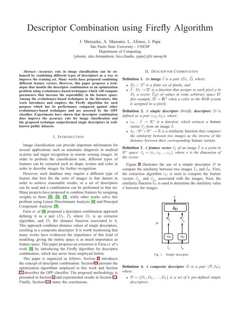
Descriptor Combination using Firefly AlgorithmJ. Matsuoka, A. Mansano, L. Afonso, J. PapaSão Paulo State University - UNESPDepartment of Computing{jekemi, alex.fernandesm, luis.claudio, papa}@fc.unesp.brAbstract—Accuracy rate in image classification can be enhancedby combining different types of descriptors as a way toimprove the training set. Many works have proposed combiningdifferent feature vectors. However, this paper proposes a techniquethat models the descriptor combination as an optimizationproblem using evolutionary-based techniques which will computeparameters that increase the separability in the feature space.Among the evolutionary-based techniques in the literature, thiswork introduces and employs the Firefly algorithm for suchpurpose which has its performance compared against otherevolutionary-based techniques and are assessed by the OPFclassifier. Experiments have shown that descriptor combinationdoes improve the accuracy rate for image classification andthe proposed technique outperformed single descriptors in wellknownpublic datasets.I. INTRODUCTIONImage classification can provide important information forseveral applications such as automatic diagnosis in medicalsystems and target recognition in remote sensing images. Inorder to perform the classification task, different types offeatures can be extracted such as shape, texture and color inorder to describe images for further recognition.However, each database may require a different type offeature that best fits the sorts of images in that dataset inorder to achieve reasonable results, or a set of descriptorscan be used and a combination can be performed in that set.Many projects have proposed to combine features by assigningweights to them [1], [2], [3], while other works solve thisproblem using Linear Discriminant Analysis [4] and PrincipalComponent Analysis [5].Faria et. al [6] proposed a descriptor combination approachdefining it as a pair (D I , ⃗ I), where DI is an extractoralgorithm, and D I the distance function associated to it.This approach combines distance values of single descriptors,resulting in a composite descriptor. It is worth mentioning thatmany works have evidenced the importance of this kind ofmodeling, giving the metric space is as much importance asfeature space. This paper proposes an extension to Faria et. al‘swork [6] by introducing the Firefly algorithm for descriptorcombination, which has never been employed before.This paper is organized as follows: Section II introducesthe concept of descriptor combination. Section III presents theoptimization algorithms employed in this work and SectionIV describes the OPF classifier. The proposed methodology ispresented in Section V and experimental results in Section VI.Finally, Section VII states the conclusions.II. DESCRIPTOR COMBINATIONDefinition 1. An image Î is a pair (D I, ⃗ I), where:• D I ⊂ Z 2 is a finite set of pixels, and• ⃗ I : D I → D ′ is a function that assigns to each pixel p inD I a vector ⃗ I(p) of values in some arbitrary space D ′(for example, D ′ = IR 3 when a color in the RGB systemis assigned to a pixel).Definition 2. A simple descriptor (briefly, descriptor) D isdefined as a pair (ǫ D ,δ D ), where:• ǫ D : Î → R n is a function, which extracts a featurevector ⃗vÎ from an image Î.• δ D : R n ×R n → R is a similarity function that computesthe similarity between two images as the inverse of thedistance between their corresponding feature vectors.Definition 3. A feature vector ⃗vÎ of an image Î is a point inR n space: ⃗vÎ = (v 1 ,v 2 ,...,v n ), where n is the dimension ofthe vector.Figure 1 illustrates the use of a simple descriptor D tocompute the similarity between two images ÎA and ÎB. First,the extraction algorithm ǫ D is used to compute the featurevectors ⃗vÎA and ⃗vÎB associated with the images. Next, thesimilarity function δ D is used to determine the similarity valued between the images.D:Fig. 1.v I^Aε DI^Adδ Dv I^Bε DI^BSimple descriptor.Definition 4. A composite descriptor ˆD is a pair (D,δ D ),where:• D = {D 1 ,D 2 ,...,D k } is a set of k pre-defined simpledescriptors.

• δ D is a similarity function which combines the similarityvalues obtained from each descriptor D i ∈ D,i = 1,2,...,k.Figure 2 illustrates the use a composite descriptor ˆD tocompute the distance between images ÎA and ÎB.D:δ Dd 1 d 2 d kδ D1 δ D2δ Dkε D ε 1 D ε 1 D ε 2 D... ε 2 D ε k D kFig. 2.I^Ad^I BComposite descriptor.III. OPTIMIZATION ALGORITHMSIn this section we briefly describe the evolutionary-basedtechniques for descriptor combination addressed in this paper:Firefly Algorithm, Harmony Search and Particle SwarmOptimization.A. Firefly AlgorithmAs most of the optimization algorithms, the Firefly algorithm(FFA) is another nature-inspired algorithm designed byYang [7]. The Firefly algorithm is a metaheuristic algorithmbased on Lévy flights and firefly’s flashing light which is usedto attract mating partners, preys and as a protective warning.Also, fireflies can imitate other fireflies’ flashing pattern inorder to attract and eat them. Lévy flights represent the flightpatterns of many animals and insects and is used in thisalgorithm to model the flight of fireflies on their search foran optimum solution.Thus, FFA explores how light intensity is used to attractother fireflies and Lévy flights for optimization problems asparticles attract each other and move toward an optimumsolution in the Particle Swarm Optimization algorithm. FFAis designed according to three rules: (i) fireflies are unisex sothat they attract each other, (ii) attractiveness is proportionalto their brightness, in which the less bright moves toward thebrighter one, and (iii) the landscape of the objective functionaffects the brightness.Light intensity and attractiveness are formulated in whichattractiveness can be associated to the firefly’s brightness andthe brightness can be associated to the solution of the problem.However, light intensity is relative to the distance between thefirefly source and the firefly that is receiving the light. Yangformulates the light intensity I(r) varying according to theinverse square law:I(r) = I sr2, (1)in which I s is the source’s intensity and r the distance.Attractiveness is proportional to the light intensity and definedas:β = β 0 e −γr2 , (2)where β 0 is the attractiveness at r = 0.So, when the firefly is near the optimum solution itsbrightness increases and attracts other fireflies which startmoving toward the brighter firefly. Their movements in thesearch space are defined by the Lévy-Flight which is randomwalks in the space (Algorithm 1).Algorithm 1. – FIREFLY ALGORITHMINPUT:OUTPUT:Set of fireflies.Best solution.1. Generate the initial population of z fireflies.2. Set light intensity I for each firefly a according to x.3. For each firefly a = 1:z4. For each firefly b = 1:z5. If I a > I b ,then6. Firefly b moves toward a using the Levy-flight.7. Evaluate the solution and update light intensity.8. Rank fireflies according to their brightness9. Return the best solution.In line 2, x stands for the location of the firefly in thespace, and fireflies are ranked (Line 8) in order to find the bestsolution. The distance between two fireflies is their respectiveCartesian distance and the movement of a fireflyato a brighterfirefly b is:x a = x a +β 0 e −γr2 ab (xb −x a )+αsign[rand− 1 ]⊕Levy, (3)2where sign[rand− 1 2] with rand ∈ [0,1] provides a randomdirection and Levy provides the lenght of the step. Also, themovement is based on the attraction (second term) and arandomization via Lévy-Flight where α is the randomizationparameter.B. Harmony SearchThe Harmony Search algorithm is an evolutionary algorithmbased on music composition, considering a process in whichmusicians improvise to create music [8]. Its main characteristicsare the simple concept, a few parameters and speed tofind a solution.The idea is to use the process of creating new songs inorder to find solutions for optimization problems, in whichsolutions are modeled as harmonies and each parameter to beoptimized is represented as a note. The final solution will bethe best harmony computed by the algorithm. The main stepsare:1) Initialize algorithm parameters;2) Initialize Harmony Memory (HM) with random values;

3) Improvise a new harmony to HM;4) Updates the HM if the new harmony is better than theworst harmony in HM, inserts the new harmony in HMand removes the worst from it;5) If the stop criteria has not been reached, return to step3.In Step 3, a new harmony vector ⃗x ′ =(x ′1 ,x ′2 ,. . . , x ′N )is generated from the HM based on memory considerations,pitch adjustments, and randomization (music improvisation).As follows:(i) position (⃗x i ) and (ii) velocity (⃗v i ). First, we define thenumber of particles that will be initialized with random valuesfor both velocity and position. Each particle is evaluated toupdate the local maximum through its fitness function. Finally,the best position is update with respect to the best of the localmaximum particles.This process is repeated until some convergence criterionis reached, i.e. number of iterations. The given particle p i hasthe velocity and position equations at time step t, respectively,given byx ′j←{x ′j ∈x ′j ∈ φ j{ }x j 1 ,xj 2 ,...,xj HMSwith probability HMCR,with probability (1-HMCR),in which φ j denotes the range of values for variable j, for φ =(φ i ,φ 2 ,...,φ N ). The HMCR is the probability of choosingone value from the historic values stored in the HM, and (1-HMCR) is the probability of randomly choosing one feasiblevalue not limited to those stored in the HM. In order to makeit clear, an HMCR=0.7 means that 70% of the notes (decisionvariables) to compose the new harmony h ′ = (⃗x ′ ) will bepicked from HM, and the remaining ones will be randomlygenerated within the interval φ j .The pitch adjustment for each harmony is often used toimprove solutions and to escape from local optimum. Thismechanism concerns shifting the neighboring values of somedecision variable in the harmony:x ′j ← x ′j +rb, (5)where x j is the note j that composes the new harmony vector,b is an arbitrary distance bandwidth for the continuous designvariable, and r is a uniform distribution between 0 and 1. Inthis paper, we set b = 1.In Step 4, if the new harmony h ′ is better than the worstharmony in the HM, the latter is replaced by this new harmony.Finally, in Step 5, the HS algorithm finishes when it satisfiesthe stopping criterion. Otherwise, Steps 3 and 4 are repeatedin order to improvise a new harmony again.C. Particle Swarm OptimizationThe Particle Swarm Optimization (PSO) algorithm wasproposed by [9] in order to find solutions for optimizationproblems. The algorithm is based on social behavior dynamicsin which each solution for a given problem is represented byparticles which “fly” in the search space.Particle Swarm Optimization (PSO) is an optimization algorithmbased on social behavior dynamics [9], that finds asolution in a search space. Each solution is modeled as aparticle in the swarm, which has a memory that stores itsbest local solution (local maxima) and the best global solution(global maxima). Each particle compares its value with theneighborhood based on a objective function, and decides ifcopies it in order to get the best local and global maxima.The swarm is modeled in a multidimensional space R N , inwhich each particle p i = (⃗x i ,⃗v i ) ∈ R N has two main features:(4)v j i (t+1) = wvj i (t)+c 1r 1 (ˆx i (t)−x j i (t))+c 2r 2 (⃗g−x j i (t)) (6)andx j i (t+1) = xj i (t)+vj i (t+1), (7)where w is the inertia weight that controls the interactionbetween particles, and r 1 ,r 2 ∈ [0,1] are random variablesthat give the stochastic idea to Particle Swarm Optimization.The variables c 1 and c 2 are used to guide the particles ontogood directions.IV. OPTIMUM-PATH FOREST CLASSIFICATIONThe OPF classifier works by modeling the problem ofpattern recognition as a graph partition in a given featurespace. The nodes are represented by the feature vectors and theedges connect all pairs of them, defining a full connectednessgraph. This kind of representation is straightforward, given thatthe graph does not need to be explicitly represented, allowingus to save memory. The partition of the graph is carried out bya competition process between some key samples (prototypes),which offer optimum paths to the remaining nodes of thegraph. Each prototype sample defines its optimum-path tree(OPT), and the collection of all OPTs defines an optimumpathforest, which gives the name to the classifier [10], [11].The OPF can be seen as a generalization of the well-knownDijkstra’s algorithm to compute optimum paths from a sourcenode to the remaining ones [12]. The main difference relieson the fact that OPF uses a set of source nodes (prototypes)with any smooth path-cost function [13]. In case of Dijkstra’salgorithm, a function that summed the arc-weights along a pathwas applied. In regard to the supervised OPF version addressedhere, we have used a function that gives the maximum arcweightalong a path, as explained below.Let Z = Z 1 ∪Z 2 ∪Z 3 be a dataset labeled with a functionλ, in which Z 1 , Z 2 and Z 3 are, respectively, a training,validation and test sets. LetS ⊆ Z 1 a set of prototype samples.Essentially, the OPF classifier creates a discrete optimumpartition of the feature space such that any sample s ∈ Z 2 ∪Z 3can be classified according to this partition. This partition isan optimum path forest (OPF) computed in R n by the ImageForesting Transform (IFT) algorithm [13].The OPF algorithm may be used with any smooth path-costfunction which can group samples with similar properties [13].Particularly, we used the path-cost function f max , which is

computed as follows:{0 if s ∈ S,f max (〈s〉) =+∞ otherwisef max (π ·〈s,t〉) = max{f max (π),d(s,t)}, (8)in which d(s,t) means the distance between samples s andt, and a path π is defined as a sequence of adjacent samples.In such a way, we have that f max (π) computes the maximumdistance between adjacent samples in π, when π is not a trivialpath.The OPF algorithm works with training and testing phases.In the former step, the competition process begins with theprototypes computation. We are interested into finding theelements that fall on the boundary of the classes with differentlabels. For that purpose, we can compute a Minimum SpanningTree (MST) over the original graph and then mark as prototypesthe connected elements with different labels. Figure 3bdisplays the MST with the prototypes at the boundary. Afterthat, we can begin the competition process between prototypesin order to build the optimum-path forest, as displayed inFigure 3c. The classification phase is conducted by takinga sample from the test set (blue triangle in Figure 3d) andconnecting it to all training samples. The distance to alltraining nodes are computed and used to weight the edges.Finally, each training node offers to the test sample a costgiven by a path-cost function (maximum arc-weight along apath - Equation 8), and the training node that has offeredthe minimum path-cost will conquer the test sample. Thisprocedure is shown in Figure 3e.0.30.41.50.40.51.10.00.91.8(a)0.01.11.40.70.70.30.40.41.10.00.9(b)0.00.90.70.7V. DESCRIPTOR COMBINATION USING FIREFLYALGORITHMMansano et. al [14] have proposed an extension to Faria’set al. work [6] by introducing a set of parameters β =(β 1 ,β 2 ,...,β M ) in order to allow a greater variability ofarithmetic computations, which was limited by the linearformulation proposed by Faria et al. [6] (Eq. 9) . Equation10 presents the proposed formulation.δ ∗ D =δ ∗ D =N∑α i δ Di , (9)i=1N∑i=1α i δ βiD i, (10)in which −2 ≤ α i ,β i ≤ 2, β i ∈ R.The optimization algorithms are responsible for computingthe best values for α and β that maximize the accuracy rateover the validation set which is our objective function. As it isknown, each agent (particle, harmony or firefly) represents adifferent solution which changes at the end of each iteration.Each pair (α, β) provides a different training set which isassessed using the validation set. The process of computingnew solutions and validation each of them repeats until thenumber of iterations is reached and the best training set of allcomputed is saved in order to run the tests. The purpose ofvalidation the training set is to obtain the set that may providethe highest accuracy rates for a given problem.Thus, the methodology uses three sets: (i) training set whichwill become the final training set, (ii) validation set usedto evaluate the descriptor combination parameters at eachiteration of the optimization algorithms, and (iii) testing setwhich is used to assess the final training set. Then, the wholeprocess can be split in two phases: (i) the design phase wherethe final training set is modeled by means of optimizationalgorithms which compute the best parameters for the set ofdescriptors, and (ii) classification phase in which each sampleis classified using the training model computed in the previousphase. Figure 4 shows the methodology proposed by Mansanoet. al [14].0.40.40.70.50.6(c)0.0(d)0.40.70.00.40.6(e)Fig. 3. OPF pipeline: (a) complete graph, (b) MST and prototypes bounded,(c) optimum-path forest generated at the final of training step, (d) classificationprocess and (e) the triangle sample is associated to the white circle class. Thevalues above the nodes are their costs after training, and the values above theedges stand for the distance between their corresponding nodes.Fig. 4. Proposed methodology for descriptor combination. Extracted fromMansano et. al [14]

VI. EXPERIMENTAL RESULTSExperiments used two well-known public datasets:• Corel 1 : It contains 3,906 images labeled in 85 classes,and the number of images per class ranges from 7 to 98images.• Free Photo 2 : A subset of this dataset was employedcontaining 3,426 images labeled in 9 classes, and thenumber of images per class ranges from 70 to 854 images.Different types of descriptors were computed for eachdataset [15]:• Color Autocorrelogram (ACC): descriptor of color representingthe space color in 64 bins and 4 values ofdistance.• Border/Interior pixel Classification (BIC): it is a descriptorof color in which color space is represented by 64bins.• Color Coherent Vector (CCV): descriptor of color composedby a combination of two histograms of 64 binstotal.• Global Color Histogram (GCH): descriptor of color inwhich the color space was split in 64 bins.• Homogeneous Texture Descriptor (HTD): descriptor oftexture• Local Activity Spectrum (LAS): descriptor of texture inwhich components are quantized in 4 bins resulting in ahistogram of 256 bins.• Quantized Compound Change Histogram (QCCH): descriptorof texture composed by 40 bins.There were computed the ACC, BIC, GCH, LAS and QCCHdescriptors for Corel dataset; and BIC, CCV, LAS, GCH andHTD for Free Photo dataset [16]The set of descriptors is split in: training, validation andtesting sets. Experiments using a single descriptor used justthe training and testing sets, and experiments involving combinationis performed using the 3 sets where the validation setis employed to evaluate the solution given by the optimizationalgorithms. The accuracy rate is computed according to Eq.11.∑ ni=1Acc =ta i, (11)nin which ta i stands for the accuracy rate of class i and nrepresents the number of classes.Table I shows the average accuracy rate of 5 rounds of testsfor each descriptor and each database using the OPF classifierusing a single descriptor.Single descriptor experiments used a training set of 30%of the entire dataset and 50% of the dataset for testing whichwere randomly generated in each round of test. The purpose ofthis first experiment is to compare the gain when descriptorcombination with optimization algorithms is performed. Resultsshow different performances for each descriptor in each1 http://vision.stanford.edu2 http://www.freefoto.comDescriptor/Dataset Corel Free PhotoACC(HTD) 74.27%±1.13 73.11%±1.31LAS 59.75%±0.60 74.58%±0.65BIC 72.67%±0.20 89.71%±0.96GCH 65.82%±0.76 78.69%±1.25QCCH(CCV) 57.38%±0.60 80.50%±0.61TABLE ISINGLE DESCRIPTOR EFFICIENCY.database where most of them had a better performance in theFree Photo database.Experiments combining different descriptors included optimizationalgorithms which were employed separately in orderto assess each algorithm’s performance. In this phase, thevalidation set is included in order to evaluate and improvethe training set prior the test step. The parameters of eachalgorithm were set as shown in Table II where there were used250 agents (fireflies, particles and harmonies), 100 iterationsand parameters with similar functions were set with the samevalue (e.g. HMCR from HS and w from PSO) in order tomake a fair comparison.Technique ParametersFFA α = 0.2, β = 1.0, γ = 1.0HS HMCR: 0.7, PAR: 0.7PSO w = 0.7, c 1 = 1.6, c 2 = 0.4TABLE IIPARAMETERS USED IN THE EXPERIMENTS.Since the purpose is to improve accuracy rate in imageclassification, the OPF classifier was employed to assess eachcombination computed by each technique and accuracy ratesfor combinations of 2 and 5 descriptors, in order words, theaccuracy rate is the objective function to be maximized. TableIII presents the mean accuracy rates for combination of 2(LAS and GCH, empirically chosen) and 5 descriptors for eachtechnique and dataset.Descriptor/Dataset Corel Free PhotoFFA-LAS+GCH 65.82%±0.86 84.48%±0.83HS-LAS+GCH 67.94%±0.74 84.28%±0.43PSO-LAS+GCH 68.04%±0.62 84.52%±0.71FFA-ALL 76.02%±1.05 90.69%±1.06HS-ALL 75.34%±0.81 89.88%±0.91PSO-ALL 76.77%±0.60 90.36%±0.72TABLE IIICOMPOSITE DESCRIPTOR EFFICIENCY ACCORDING TO THE PROPOSEDAPPROACH.Comparing the combination of 2 and 5 descriptors, it isvisible an improvement of over 8% in Corel database andalmost 6% in the Free Photo, considering the best accuracyrates in each scenario. Among the optimization algorithms,PSO has achieved the best accuracy rates in 3 out of 4situations, although all techniques had similar results.However, comparing performances of single descriptor anddescriptor combination using 5 descriptors has shown a slight

difference of over 2% for Corel database and almost 1% forFree Photo database. The low gain might be caused due tothe usage of a descriptor that has low performance in suchconfiguration of datasets.VII. CONCLUSIONSMany approaches have proposed feature combination in imageclassification. This paper has presented techniques basedon social dynamics to perform descriptor combination usingoptimization algorithms and Firefly Algorithm is introduced inthis context, which is defined by a pair of feature extractionalgorithm and a distance function associated with it.The approach consists in a mathematical formulation of acomposite descriptor, which is obtained by combining descriptorsusing PSO, HS and FFA, and the OPF to perform the tests.In this case, the accuracy rate of OPF in a validation set is usedas an objective function to be maximized by these techniques.Experiments with color and texture features have shown thatcombining different descriptors can outperform the sensibilityin image classification.[13] A.X. Falcão, J. Stolfi, and R.A. Lotufo, “The image foresting transformtheory, algorithms, and applications,” IEEE Transactions on PatternAnalysis and Machine Intelligence, vol. 26, no. 1, pp. 19–29, 2004.[14] A. Mansano, J. A. Matsuoka, L. C S Afonso, J. P. Papa, F. Faria, andR. da S Torres, “Improving image classification through descriptorcombination,” in Graphics, Patterns and Images (SIBGRAPI), 201225th SIBGRAPI Conference on, 2012, pp. 324–329.[15] F. A. Faria, J. A. dos Santos, A. Rocha, and R. S. Torres, “Automaticclassifier fusion for produce recognition.,” in SIBGRAPI. 2012, pp. 252–259, IEEE Computer Society.[16] O.A.B. Penatti, E. Valle, and R.S. Torres, “Comparative study of globalcolor and texture descriptors for web image retrieval,” J. of VisualCommunication and Image Representation, 2011.VIII. ACKNOWLEDGMENTSThe authors thank FAPESP (Procs. #2011/11777-0,#2012/09809-4 and #2009/16206-1) and CNPq grant#303182/2011-3.REFERENCES[1] P. Gehler and S. Nowozin, “On feature combination for multiclass objectclassification,” in Proceedings of the 12th International Conference onComputer Vision, 2009, pp. 221–228.[2] J. Hou, B.-P. Zhang, N.-M. Qi, and Y. Yang, “Evaluating feature combinationin object classification,” in Proceedings of the 7th InternationalConference on Visual Computing, Las Vegas, NV, USA, 2011, pp. 597–606, Springer-Verlag.[3] D. Okanohara and J. Tsujii, “Learning combination features with L1regularization,” in Proceedings of Human Language Technologies: The2009 Annual Conference of the North American Chapter of the ACL,Stroudsburg, PA, USA, 2009, pp. 97–100.[4] X. Liu, L. Zhang, M. Li, H. Zhang, and D.Wang, “Boosting image classificationwith LDA-based feature combination for digital photographmanagement,” Pattern Recognition, vol. 38, no. 6, pp. 887–901, June2005.[5] F. Yan and X. Yanming, “Image classification based on multi-featurecombination and PCA-RBaggSVM,” in Proceedings of the IEEEInternational Conference on Progress in Informatics and Computing,2010, vol. 2, pp. 888–891.[6] F.A. Faria, J.P. Papa, R.S. Torres, and A.X. Falcão, “Multimodalpattern recognition through particle swarm optimization,” in Proceedingsof the 17th International Conference on Systems, Signals and ImageProcessing, Rio de Janeiro, Brazil, 2010, pp. 1–4.[7] Xin-She Yang, “Firefly algorithm, lévy flights and global optimization,”in SGAI Conf., 2009, pp. 209–218.[8] Z. Geem, “Novel derivative of harmony search algorithm for discretedesign variables,” Applied Mathematics and Computation, vol. 199, no.1, pp. 223–230, May 2008.[9] J. Kennedy and R.C. Eberhart, Swarm Intelligence, M. Kaufman, 2001.[10] J. P. Papa, A. X. Falcão, and C. T. N. Suzuki, “Supervised patternclassification based on optimum-path forest,” International Journal ofImaging Systems and Technology, vol. 19, no. 2, pp. 120–131, 2009.[11] J. P. Papa, A. X. Falcão, V. H. C. Albuquerque, and J. M. R. S.Tavares, “Efficient supervised optimum-path forest classification forlarge datasets,” Pattern Recognition, vol. 45, no. 1, pp. 512–520, 2012.[12] E. W. Dijkstra, “A note on two problems in connexion with graphs,”Numerische Mathematik, vol. 1, pp. 269–271, 1959.