Estimating Cleanup Times Associated with Combining Source-Area ...

ENGINEERING SERVICE CENTERPort Hueneme, California 93043-4370TECHNICAL REPORTTR-2288-ENVESTIMATING CLEANUP TIMES ASSOCIATEDWITH COMBINING SOURCE-AREAREMEDIATION WITH MONITORED NATURALATTENUATIONPrepared by:Mark Widdowson, Phd, PE, Virginia TechFrancis Chapelle, Phd, United States Geological SurveyClifton Casey, PE, NAVFAC SOUTHMark Kram, Phd, NAVFAC ESCFebruary 2008Approved for public release; distribution is unlimited.

Form ApprovedREPORT DOCUMENTATION PAGEOMB No. 0704-0811The public reporting burden for this collection of information is estimated to average 1 hour per response, including the time for reviewing instructions, searching existing data sources, gathering andmaintaining the data needed, and completing and reviewing the collection of information. Send comments regarding this burden estimate or any other aspect of this collection of information, includingsuggestions for reducing the burden to Department of Defense, Washington Headquarters Services, Directorate for Information Operations and Reports (0704-0188), 1215 Jefferson Davis Highway,Suite 1204, Arlington, VA 22202-4302. Respondents should be aware that notwithstanding any other provision of law, no person shall be subject to any penalty for failing to comply with a collection ofinformation, it if does not display a currently valid OMB control number.PLEASE DO NOT RETURN YOUR FORM TO THE ABOVE ADDRESS.1. REPORT DATE (DD-MM-YYYY) 2. REPORT TYPE 3. DATES COVERED (From – To)12-FEBRUARY-2008 Technical Report 14-August-2008 to 12 February-20084. TITLE AND SUBTITLE 5a. CONTRACT NUMBERESTIMATING CLEANUP TIMES ASSOCIATED WITH COMBININGSOURCE-AREA REMEDIATION WITH MONITORED NATURALATTENUATIONN47408-04-C-75245b. GRANT NUMBER5c. PROGRAM ELEMENT NUMBER6. AUTHOR(S) 5d. PROJECT NUMBERMark Widdowson, Phd, PE, Virginia TechFrancis Chapelle, Phd, United States Geological SurveyClifton Casey, PE, NAVFAC SOUTHMark Kram, Phd, NAVFAC ESCESTCP ER-04365e. TASK NUMBER5f. WORK UNIT NUMBER7. PERFORMING ORGANIZATION NAME(S) AND ADDRESSES 8. PERFORMING ORGANIZATION REPORT NUMBERNaval Facilities Engineering Service Center1100 23 rd AvenuePort Hueneme, CA 93043TR-2288-ENV9. SPONSORING/MONITORING AGENCY NAME(S) AND ADDRESS(ES) 10. SPONSOR/MONITORS ACRONYM(S)Environmental Security Technology Certification Program901 North Stuart Street, Suite 303Arlington, VA 2220312. DISTRIBUTION/AVAILABILITY STATEMENTApproved for public release; distribution is unlimited.ESTCP11. SPONSOR/MONITOR’S REPORT NUMBER(S)13. SUPPLEMENTARY NOTES14. ABSTRACTUnder suitable conditions, monitored natural attenuation (MNA) can be a cost-effective strategy for restoring contaminated aquifer systems eitheras a stand-alone technology or in combination with other engineered remedial actions. However, USEPA guidance specifically requires MNA toachieve site-specific cleanup objectives within a reasonable time frame. Thus, it is necessary to provide estimates of cleanup times whenever MNAis proposed as part of a cleanup strategy.In response, the Natural Attenuation Software (NAS) was co-developed by the Naval Facilities Engineering Command (NAVFAC), U.S.Geological Survey (USGS), and Virginia Tech. NAS is a screening tool designed for estimating time of remediation (TOR) for MNA with varyingdegrees of source area remediation. Conventional screening tools for MNA are not designed to address source zone remediation options orsimulation of plume reduction. The NAS consists of a combination of computational tools implemented in three main interactive modules toprovide estimates for: 1) target source concentration required for a plume extent to contract to regulatory limits, 2) time required for contaminants inthe source area to attenuate to a predetermined target source concentration, and 3) time required for a plume extent to contract to regulatory limitsafter source reduction. Natural attenuation processes that NAS models include are advection, dispersion, sorption, non-aqueous phase liquid(NAPL) dissolution, and biodegradation of petroleum hydrocarbons, chlorinated solvents, or any user-specified contaminants or mixtures. NAScan also be used to determine the equilibrium concentrate at any given location following source-zone remediation and when this will occur.15. SUBJECT TERMSNAS, MNA, TOR, source area, source-zone, NAPL, DNAPL, LNAPL, remediation, groundwater16. SECURITY CLASSIFICATION OF: 17. LIMITATION OF 18. NUMBER OF 19a. NAME OF RESPONSIBLE PERSONa. REPORT b. ABSTRACT c. THIS PAGEABSTRACTPAGESU U U 192Dr. Mark Kram19b. TELEPHONE NUMBER (include area code)805-982-2669Standard Form 298 (Rev. 8/98)Prescribed by ANSI Std. Z39.18iii

(This page is left intentionally blank)vi

TABLE OF CONTENTSLIST OF TABLES .............................................................................................................................. ixLIST OF FIGURES ............................................................................................................................. ixLIST OF APPENDICES...................................................................................................................... xiiACRONYMS.................................................................................................................................... xiiACKNOWLEDGEMENTS.................................................................................................................. xivEXECUTIVE SUMMARY................................................................................................................... xv1. Introduction............................................................................................................................. 11.1. Background..................................................................................................................... 11.2. Objectives of the Demonstration .................................................................................... 11.3. Regulatory Drivers.......................................................................................................... 21.4. Stakeholder Issues........................................................................................................... 22. Technology Description.......................................................................................................... 32.1. Technology Description and Application ....................................................................... 32.2. Previous Testing of the Technology ............................................................................... 82.3. Factors Affecting Cost and Performance........................................................................ 82.4. Advantages and Limitations of the Technology ............................................................. 83. Demonstration Design .......................................................................................................... 103.1. Performance Objectives................................................................................................ 103.2. Selection of Test Sites................................................................................................... 123.3. Test Site Description..................................................................................................... 143.3.1. Seneca Army Depot, NY – Ash Landfill.................................................................. 143.3.1.1. History of Operations............................................................................................ 143.3.1.2. Site Hydrogeology ................................................................................................ 153.3.1.3. Source and Plume Description.............................................................................. 153.3.1.4. Redox Conditions ................................................................................................. 173.3.1.5. Past and Current Remediation Approaches .......................................................... 173.3.2. Niagara Falls, NY – USGS Site................................................................................ 173.3.2.1. History of Operations............................................................................................ 173.3.2.2. Site Hydrogeology ................................................................................................ 183.3.2.3. Source and Plume Description.............................................................................. 183.3.2.4. Redox Conditions ................................................................................................. 203.3.2.5. Past and Current Remediation Approaches .......................................................... 213.3.3. NAES Lakehurst, NJ – Sites I&J.............................................................................. 213.3.3.1. History of Operations............................................................................................ 213.3.3.2. Site Hydrogeology ................................................................................................ 213.3.3.3. Source and Plume Description.............................................................................. 223.3.3.4. Redox Conditions ................................................................................................. 233.3.3.5. Past and Current Remediation Approaches .......................................................... 233.3.4. Hill AFB, UT – OU2 ................................................................................................ 233.3.4.1. History of Operations............................................................................................ 233.3.4.2. Site Hydrogeology ................................................................................................ 253.3.4.3. Source and Plume Description.............................................................................. 253.3.4.4. Redox Conditions ................................................................................................. 26vii

3.3.4.5. Past and Current Remediation Approaches .......................................................... 263.3.5. NSB Kings Bay, GA – Site 11.................................................................................. 273.3.5.1. History of Operations............................................................................................ 273.3.5.2. Site Hydrogeology ................................................................................................ 273.3.5.3. Source and Plume Description.............................................................................. 273.3.5.4. Redox Conditions ................................................................................................. 273.3.5.5. Past and Current Remediation Approaches .......................................................... 283.3.6. NAS Cecil Field, FL – Site 3.................................................................................... 293.3.6.1. History of Operations............................................................................................ 293.3.6.2. Site Hydrogeology ................................................................................................ 293.3.6.3. Source and Plume Description.............................................................................. 313.3.6.4. Redox Conditions ................................................................................................. 313.3.6.5. Past and Current Remediation Approaches .......................................................... 313.3.7. NAS Pensacola, FL – WWTP................................................................................... 323.3.7.1. History of Operations............................................................................................ 323.3.7.2. Site Hydrogeology ................................................................................................ 323.3.7.3. Source and Plume Description.............................................................................. 323.3.7.4. Redox Conditions ................................................................................................. 343.3.7.5. Past and Current Remediation Approaches .......................................................... 343.3.8. Alaska DOT&PF – USGS (Peger Road) Site........................................................... 353.3.8.1. History of Operations............................................................................................ 353.3.8.2. Site Hydrogeology ................................................................................................ 353.3.8.3. Source and Plume Description.............................................................................. 353.3.8.4. Redox Conditions ................................................................................................. 363.3.8.5. Past and Current Remediation Approaches .......................................................... 363.4. Pre-Demonstration Testing and Analysis ..................................................................... 363.5. Testing and Evaluation Plan ......................................................................................... 373.6. Selection of Analytical/Testing Methods...................................................................... 373.7. Selection of Analytical/Testing Laboratory.................................................................. 374. Performance Assessment ...................................................................................................... 384.1. Performance Criteria..................................................................................................... 384.2. Performance Confirmation Methods............................................................................. 394.3. Data Analysis, Interpretation and Evaluation ............................................................... 404.3.1. Seneca Army Depot, NY – Ash Landfill.................................................................. 414.3.2. Niagara Falls, NY – USGS Site................................................................................ 424.3.3. NAES Lakehurst, NJ – Sites I&J.............................................................................. 444.3.4. Hill AFB, UT – OU2 ................................................................................................ 464.3.5. NSB Kings Bay, GA – Site 11.................................................................................. 474.3.6. NAS Cecil Field, FL – Site 3.................................................................................... 484.3.7. NAS Pensacola, FL – WWTP................................................................................... 514.3.8. Alaska DOT&PF – USGS (Peger Road) Site........................................................... 514.4. Overall Performance Assessment ................................................................................. 554.4.1. Accuracy ................................................................................................................... 554.4.2. Versatility.................................................................................................................. 564.4.3. Reliability.................................................................................................................. 56viii

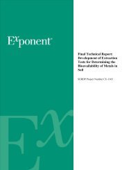
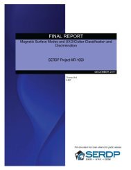
4.4.4. Applicability ............................................................................................................. 565. Cost Assessment ................................................................................................................... 575.1. Cost Reporting .............................................................................................................. 575.2. Cost Analysis ................................................................................................................ 585.2.1. Life Cycle Cost Analysis .......................................................................................... 585.2.2. Implementation Cost Analysis.................................................................................. 586. Implementation Issues .......................................................................................................... 616.1. Environmental Checklist............................................................................................... 616.2. Other Regulatory Issues................................................................................................ 616.3. End-User Issues ............................................................................................................ 617. References............................................................................................................................. 618. Points of Contact................................................................................................................... 65LIST OF TABLESTable 1. Locations of Demonstrations...........................................................................................2Table 2. Summary of NAS v2.2 Site Data Requirements.............................................................. 6Table 3. Performance Objectives................................................................................................. 12Table 4. Performance Criteria...................................................................................................... 38Table 5. Performance and Performance Confirmation Methods ................................................. 39Table 6. Summary of TOR Component Tested for each Site Application .................................. 40Table 7. Comparison of Experimentally-Derived and NAS-Derived Rate Constants................. 53Table 8. Basis for NAS Cecil Field Life Cycle Cost Estimates................................................... 57Table 9. Estimated Cost for MNA at Site 3................................................................................. 58Table 10. Estimated Costs for Performing a TOR Analysis Using NAS or a ComprehensiveNumerical Model at a Hypothetical Site. ..................................................................... 59Table 11. Cost Comparison and Savings for Two Hypothetical Sites of Differing Size............. 60LIST OF FIGURESFigure 1. Flowchart showing how the NAS software can be applied to TOR problems............... 7Figure 2. Measured versus NAS-simulated concentration changes at well KBA-11-13A. Points(A1) and (A2) are inflection points, (B) is located at the time of breakthrough and (C)indicates the slope of the concentration decline. .......................................................... 11Figure 3. Measured versus NAS-simulated concentration changes at well MW-8. .................... 11Figure 4. Location map for eight selected sites. (Source: www.nationalatlas.gov)................... 14Figure 5. Site map of Ash Landfill at the Seneca Army Depot, NY (Source: ParsonsEngineering, 2004. Final Record of Decision for Ash Landfill at Seneca Army DepotActivity, Romulus, NY (Contract Number: DACA87-95-D-0031).)........................... 16Figure 6. Map of USGS study site in Niagara Falls, NY (Yager 2002). ..................................... 19Figure 7. Vertical section A-A’ through the chlorinated ethene plume (Yager 2002). ............... 20ix

Figure 8. Site map of Areas I and J at NAES Lakehurst, NY. (Source: Dames and Moore. 1999.Final Report – Groundwater Natural Restoration Study, Areas I and J. ContractNumber N62472-90-D-1298). ...................................................................................... 22Figure 9. Site map of OU2 at Hill AFB Ogden, UT (Source: Air Force Center forEnvironmental Excellence. 2003. Conceptual Model Update for Operable Unit 2Source Zone: Hill Air Force Base, Utah). .................................................................... 24Figure 10. OU2 source area (Air Force Center 2003). ................................................................ 25Figure 11. Chloroethene plume and monitoring wells at Site 11, NSB Kings Bay. (Chapelle,F.H., P.M. Bradley, and C.C. Casey, 2005. Behavior of a chlorinated ethene plumefollowing source-area treatment with Fenten’s reagent. Ground Water Monitoring andRemediation, 25(2): 131-141). ..................................................................................... 28Figure 12. Site map of Site 3 at NAS Cecil Field, FL. (Source: NAVFAC report, 2006). ....... 30Figure 14. Aerial photo of the USGS (Peger Road) study site in Fairbanks, AK. (Source: U.S.Geological Survey, 2005. Chloroethene biodegradation potential in the "lower"contaminant plume, River Terrace RV Park, Soldotna, Alaska, U.S. Geological SurveyOpen-File Report 2004-1427)....................................................................................... 36Figure 15. Well location map for the USGS study site in Fairbanks, AK (ADEC 2005). (Source:Alaska Department of Environmental Conservation, 2005. ADOT&PF Peger RoadMaintenance Facility, Fairbanks, Alaska). ................................................................... 37Figure 16. Observed and NAS-simulated TCE concentration versus distance along plumecenterline prior to source concentration reduction. ...................................................... 41Figure 17. Observed and NAS-simulated TCE concentration versus time at downgradient wellsbased on the observed source concentration reduction................................................. 42Figure 18: NAS-calculated vs. observed TCE – Average saturated thickness =6.75 ft. ............. 43Figure 19. NAS-calculated vs. observed TCE - Average saturated thickness =3.50 ft. .............. 43Figure 20. Observed concentrations of total chlorinated ethenes for single-component sourcemodels using NAS and RT3D. A data regression is also shown................................. 44Figure 21. NAS-simulated versus observed concentrations of TCE (top), DCE (middle), andtotal chlorinated ethenes (bottom) for the multi-component source model.................. 45Figure 22. TCE concentration vs. time at wells downgradient of the slurry wall based onhydraulic gradient near the source (left) and further downgradient (right).................. 46Figure 23. Observed (circles) and predicted total chlorinated ethene concentrations showing thefull range of ground-water velocity and retardation factor values based on initialestimates made prior to the source zone treatment....................................................... 47Figure 24. Observed and NAS-predicted total chlorinated ethene concentrations using groundwatervelocity (v = 0.055 m/d) determined from the tracer breakthrough and the rangeof retardation factors, including the case (R = 2.28) where the error is minimized. .... 48Figure 25. Observed versus NAS-simulated concentrations in the source zone for three sourcemass estimates. ............................................................................................................. 49Figure 26. Observed versus NAS-simulated concentrations in the source zone for three velocityestimates. ......................................................................................................................50Figure 27. Concentrations of total chlorinated benzenes (top), benzene (middle), and 1-3dichlorobenzene (bottom) over time at well SMW-8 following ORC treatment of thesource............................................................................................................................ 52Figure 28. TCE plume centerline concentration profile and redox conditions............................ 54x

Figure 29. NAS simulation of time of stabilization at well MW98-17. ...................................... 54Figure 30. Cost savings using NAS over a 5-year period, beginning with 12 sites in Year 1, 24sites in Year 2, and 48 sites in Year 3-5. The ratio of small sites to large sites is 4:1. 60xi

LIST OF APPENDICESAppendix A: Seneca Army Depot, NY – Ash Landfill ........................................................ A-1Appendix B: Niagara Falls, NY – USGS (Textron) Site...................................................... B-1Appendix C: NAES Lakehurst, NJ – Sites I & J .................................................................. C-1Appendix D: Hill AFB, UT – OU2....................................................................................... D-1Appendix E: NSB Kings Bay, GA – Site 11 ........................................................................ E-1Appendix F: NAS Cecil Field, FL – Site 3........................................................................... F-1Appendix G: NAS Pensacola, FL – WWTP......................................................................... G-1Appendix H: Alaska DOT&PF – USGS (Peger Road) Site ................................................. H-1ACRONYMSADECADOT&PFAFBARARBGSBRACCERCLACVOCDCEDNAPLDODoDDOSERAESTCPFDEPMCASMCLMCLGMNANAESNAPLNASNASCFNAVFACNCPNPLNSBAlaska Department of Environmental ConservationAlaska Department of Transportation and Public FacilitiesAir Force Baseapplicable or relevant and appropriate requirementsbelow ground surfaceBase Realignment and ClosuresComprehensive Environmental Response, Compensation, and Liability Actchlorinated volatile organic compoundDichloroethenedense non-aqueous phase liquiddissolved oxygenDepartment of Defensedistance of plume stabilizationengineered remedial actionEnvironmental Security Technology Certification ProgramFlorida Department of Environmental ProtectionMarine Corps Air Stationmaximum contaminant levelmaximum contaminant level goalsMonitored Natural AttenuationNaval Air Engineering Stationnon-aqueous phase liquidNatural Attenuation SoftwareNaval Air Station Cecil FieldNaval Facilities Engineering CommandNational Contingency PlanNational Priority ListNaval Submarine Basexii

ORCOUPCBPCERI/FSRITSRFIRODRPMSDWASEAM3DSEDASISVOCTCATCETEAPTNDTORTOSUSEPAUSGSVCVOCWWTPoxygen release compoundOperational Unitpolychlorinated biphenyltetrachloroetheneRemedial Investigation/Feasibility StudyRemediation Innovative Technology SeminarRCRA Facility InvestigationRecord of Decisionremedial project managerSafe Drinking Water ActSequential Electron Acceptor Model, 3D transportSeneca Army Depot Activitysurface impoundmentsemi-volatile organic compoundstrichloroethanetrichloroetheneterminal electron acceptor processestime of NAPL dissolutiontime of remediationtime of plume stabilizationUnited States Environmental Protection AgencyUnited States Geological Surveyvinyl chloridevolatile organic compoundwaste-water treatment plantxiii

ACKNOWLEDGEMENTSThis work was supported by the Environmental Security Technology Certification Program(ESTCP) of the U.S. Department of Defense, as part of Project CU-0436 and through the NavalFacilities Engineering Command (NAVFAC). Andrea Leeson was the ESTCP EnvironmentalRestoration Program Manager. Dr. Mark Kram (PI), Naval Facilities Engineering CommandEngineering Service Center (NAVFAC ESC), provided technical review and was responsible forproject management. Dr. Mark Widdowson (Virginia Tech), Dr. Francis Chapelle (USGS), andClifton Casey (NAVFAC SOUTH) served as project co-PIs. They are co-authors of NAS andwere responsible for documenting the site applications and demonstration of NAS. EduardoMendez III (Virginia Tech) and Dr. J. Steven Brauner (Parsons Engineering and formerly,Virginia Tech) are also co-authors of NAS. Virginia Tech graduate students Erin Maloney andEduardo Mendez III and Virginia Tech research associate Cristhian Quezada contributed to thesite applications. The PIs wish to acknowledge all parties who provided site data and reports forthe NAS applications.xiv

EXECUTIVE SUMMARYUnder suitable conditions, monitored natural attenuation (MNA) can be a cost-effective strategyfor restoring contaminated aquifer systems either as a stand-alone technology or in combinationwith other engineered remedial actions. However, USEPA guidance specifically requires MNAto achieve site-specific cleanup objectives within a reasonable time frame. Thus, it is necessaryto provide estimates of cleanup times whenever MNA is proposed as part of a cleanup strategy.In response, the Natural Attenuation Software (NAS) was co-developed by the Naval FacilitiesEngineering Command (NAVFAC), U.S. Geological Survey (USGS), and Virginia Tech. NASis a screening tool designed for estimating time of remediation (TOR) for MNA with varyingdegrees of source area remediation. Conventional screening tools for MNA are not designed toaddress source zone remediation options or simulation of plume reduction. The NAS consists ofa combination of computational tools implemented in three main interactive modules to provideestimates for: 1) target source concentration required for a plume extent to contract to regulatorylimits, 2) time required for contaminants in the source area to attenuate to a predetermined targetsource concentration, and 3) time required for a plume extent to contract to regulatory limits aftersource reduction. Natural attenuation processes that NAS models include are advection,dispersion, sorption, non-aqueous phase liquid (NAPL) dissolution, and biodegradation ofpetroleum hydrocarbons, chlorinated solvents, or any user-specified contaminants or mixtures.NAS can also be used to determine the equilibrium concentrate at any given location followingsource-zone remediation and when this will occur.The objective of this demonstration was to evaluate the NAS software capability to providereasonable estimates of MNA cleanup timeframes in a variety of environments and sitesthroughout the United States. The tool is evaluated by using data from eight sites with long-termmonitoring data that encompass diverse geologic and hydrogeochemical environments andvarious engineered remedial actions (ERA). Results were judged based on accuracy, versatility,reliability, and applicability. The objective of the project was to validate NAS using a consistentset of procedures for comparing predicted and observed TOR results. Sites were selected torepresent a range of different hydrologic settings and ERAs. The eight demonstration sites arelocated at Seneca Army Depot and a USGS study site in New York, NAES Lakehurst in NewJersey, Hill AFB in Utah, NSB Kings Bay in Georgia, Naval Air Station Cecil Field and NavalAir Station Pensacola in Florida and a USGS study site in Alaska.The distance/time of stabilization (DOS/TOS) feature of NAS was tested at 5 sites and the timeof NAPL dissolution (TND) feature was tested at the remaining 3 test sites. Overall, theDOS/TOS feature was satisfactory in meeting quantitative and qualitative performanceobjectives based on the match between NAS and the data inflection points and concentrationversus time slopes, respectively. NAS was effective in predicting the time of stabilization ofconcentrations at monitoring wells located relatively close to the source (up to 700 ftdowngradient) following source remediation and a subsequent reduction in groundwatercontaminant concentrations in the source zone. Factors affecting the degree of accuracy werereflected in the uncertainty associated with the contaminant velocity estimates and sourcecharacteristics (width and concentration) following remediation. The TND feature wasxv

satisfactory in meeting the qualitative performance objective associated with source zones. NASwas effective in capturing concentration time trends of natural source depletion of a multicomponentNAPL, providing a prediction that was superior to a comprehensive numerical modelthat was not based on source zone mass balance.One finding of this demonstration was that NAS proved to be applicable to all eight sites,independent of hydrogeology, contaminants, characteristics of the source zone, or ERA.Therefore, the simplifying assumptions associated with the analytical solutions and the numericalsource zone model do not appear to render NAS ineffective but, in fact, demonstrate theapplicability and utility of NAS to a wide range of contaminated sites. In contrast,comprehensive three-dimensional numerical models that are constructed to simulate thecomplexities of a groundwater system and features of a plume often are subject to limited dataand may include unrealistic boundary conditions that do not honor the actual field conditions.However, there are many sites where complex hydrogeology, highly non-uniform groundwaterflow, and the desire to simulate complicated remediation strategies will dictate the use of acomprehensive numerical model.NAS, a methodology and tool for estimating the time of remediation associated with MNA, willallow stakeholders to make informed decisions regarding its application. In addition, budgetrequirements for long term monitoring programs can be forecasted based on estimates oftimeframes. This allows better program planning to meet the future needs of cleanup programs,and can afford remedial project managers (RPM) the ability to conduct cost benefit analyseswhen comparing source removal with MNA options to MNA-only strategies. The estimated costof implementing NAS was compared to cost estimates using a comprehensive numerical modelat a site to address the TOR question. The estimated cost of implementing a comprehensivenumerical model was 5.6 times greater than the estimated cost of using NAS. It is reasonable toassume that this ratio will be even greater when overhead and costs associated with oversight bysenior technical experts and regulating agencies are included.xvi

1. Introduction1.1. BackgroundMonitored Natural Attenuation (MNA) is a remedial alternative recognized by the United StatesEnvironmental Protection Agency (USEPA) that relies on naturally occurring processes toachieve site-specific remediation objectives within a time frame that is reasonable whencompared to other alternatives (USEPA 1999). The cleanup timeframe is defined as a period oftime during which the quality of ground-water will achieve a certain level at a specific location(USEPA 2001). A precursor, therefore to selection of MNA as a viable remedy requires aquantitative estimate of the time to reach remediation objectives. Estimating the cleanup timeassociated with MNA requires evaluation of a variety of physical, chemical and biologicalattenuation mechanisms. To estimate cleanup timeframes based on these processes, a screeninglevel tool is needed that can be used by project scientists and engineers to make informeddecisions during remedy selection.At sites where simplifying assumptions related to ground-water flow and transport can be made,a computational model can be used to estimate the behavior of plumes and source zones whereMNA is being considered. The Naval Facilities Engineering Command (NAVFAC), SouthernDivision, partnered with the United States Geological Survey (USGS, South Carolina District)and Virginia Polytechnic Institute and State University (Virginia Tech) to develop a screeninglevel modeling tool to estimate the site-specific cleanup time for MNA. The result of thatcollaboration was the development of the Natural Attenuation Software (NAS) funded byNAVFAC. This tool was designed to evaluate plume dynamics such as the projected plumelength, the time for the plume to stabilize, the time required for the plume to attenuate as well asestimates of the cleanup timeframes following an engineered remedial application (ERA) toremove the contaminant source, including non-aqueous phase liquids (NAPL). When used inconjunction with ERAs of source zones, MNA may be considered as a part of a combinedremedy. Under these circumstances, NAS can be used to establish nonzero cleanup thresholdsfor actively engineered remedies in the source area that will meet time, distance and exposureconstraints of the project. Although NAS had been previously applied to data from several fieldsites, there is a need to demonstrate and validate this enhanced NAS approach by comparingmodel predictions to field observations from sites representing a wide-range of conditions.1.2. Objectives of the DemonstrationThe objective of this demonstration is to evaluate the capability of the NAS software to providereasonable estimates of MNA cleanup timeframes in a variety of environments and sitesthroughout the United States. The tool is evaluated by using data from eight sites with long-termmonitoring data that encompass diverse geologic and hydrogeochemical environments anddifferent remediation options. An evaluation of predictions from early data sets with empirical1

data during the predicted period is used to make assessments of the utility of the estimates.Table 1 lists the scope and locations of the demonstrations.Table 1. Locations of DemonstrationsFacility Site Location Contaminant(s)Seneca Army Depot Ash Landfill Romulus, NY Chlorinated ethenesTextron USGS Site Niagara Falls, NY Chlorinated ethenesNAES Lakehurst Sites I & J Lakehurst, NY Chlorinated ethenesHill Air Force Base OU2 Ogden, UT Chlorinated ethenesNaval Submarine Site 11 Kings Bay, GA Chlorinated ethenesBase Kings BayNaval Air StationCecil FieldSite 3 Jacksonville, FL Chlorinated ethenes andchlorinated benzenesNaval Air StationPensacolaWWTP Pensacola, FL Chlorinated ethenes andchlorinated benzenesADOT&PF USGS Site Fairbanks, AK Chlorinated ethenes1.3. Regulatory DriversRemedial actions at Comprehensive Environmental Response, Compensation, and Liability Act(CERCLA) sites must be protective of human health and the environment and comply withapplicable or relevant and appropriate requirements (ARAR). Drinking water standards providerelevant and appropriate cleanup levels for ground-waters that are a current or potential source ofdrinking water. Drinking water standards include federal maximum contaminant levels (MCL)and/or non-zero maximum contaminant level goals (MCLG) established under the Safe DrinkingWater Act (SDWA), or more stringent state drinking water standards. Selection of MNA as aremedy for cleanup of hazardous substances requires that estimates of time of cleanup be madeto assess its feasibility as a remedy.1.4. Stakeholder IssuesStakeholder buy-in is evident by the support provided by Navy Engineering Field Divisions.This is exemplified by the recently funded NAS upgrade to allow for incorporation of a sourceremoval term. Earlier versions of NAS have been the subject of Navy supported conferencepresentations (e.g., the annual RPM Conference) and a RITS course module. End-user concerns,reservations, and buy-in factors all point to the remedial project managers’ (RPM) willingness toutilize the NAS approach versus a more comprehensive modeling effort. Concerns withimplementation have been addressed through the NAS site applications using feedback fromusers during this demonstration.2

2. Technology Description2.1. Technology Description and ApplicationOverview of Monitored Natural AttenuationMonitored natural attenuation is the considered use of naturally occurring contaminantdegradation/dispersion/immobilization processes to reach site-specific remediation goals(USEPA 1996; 1998). In current engineering practice, the effectiveness of MNA is evaluated ona site-by-site basis by considering three lines of evidence: (1) historical monitoring data showingdecreasing concentrations and/or contaminant mass over time, (2) geochemical data showing thatsite conditions favor contaminant transformation or immobilization, or (3) site-specificlaboratory studies documenting ongoing biodegradation processes (USEPA 1998). A variety offield and laboratory methods for assessing these three lines of evidence have been developed andare currently in use (Wiedemeier et al. 1999).More recently, it has been pointed out that these “lines of evidence” reflect the more generalprinciple of mass balance (USDOE 2003). If, for example, the capacity of a ground-watersystem to attenuate contaminants exceeds the mass loading of contaminants to that system, thenthe efficiency of MNA is considered relatively high (Line of evidence #1). Conversely, if thedelivery of contaminants exceeds this natural attenuation capacity, then the efficiency of MNA isproportionally lower. In either case, this contaminant loading/attenuation balance is affected byambient geochemical conditions (Line of evidence #2) and can be assessed by laboratory studiesas well as field studies (Line of evidence #3). The successful implementation of MNA requires aquantitative assessment of how contaminant mass loading is balanced by the natural attenuationcapacity of a given system relative to site-specific remediation objectives.Time of Remediation Associated with Natural AttenuationIn concept, estimating the length of time required for natural processes to remove a particularcontaminant from a ground-water system is a simple mass balance problem. If the initial mass ofcontaminant, M o , (units of mass) present in a ground-water system is known, and if the rate thatthe contaminant is transformed or destroyed by natural attenuation processes, R NA , (units of massremoved per unit time) is known, a mass balance equation can be writtenM( t ) = Mot− ∫ Rin which t is time and M ( t ) is the contaminant mass remaining at any time t. It follows that atime of remediation can be defined as the time required to lower contaminant mass below a giventhreshold (M*):0NAdt(1)3

M*= Mo*t− ∫ Rwhere the t* is time of remediation (TOR) is defined explicitly as given in Equation (2), andrefers to the length of time needed for a given mass of initial contaminant (M o ) to be loweredbelow a given regulatory threshold (M*), by the rate of natural attenuation processes (R NA )occurring in a ground-water system.In addition to providing a working definition of TOR, Equation (2) also indicates the kinds ofinformation necessary to make remediation time estimates. This information includes anestimate of the mass of contaminant present, and an estimate of the rate of ongoing naturalattenuation processes acting on the contaminant. The principal technical problem, therefore, is toobtain reliable estimates of these parameters. Clearly, the reliability of any remediation timeestimates will be directly linked to the reliability of the parameter estimates. In addition,Equation (2) shows that determining remediation times requires the definition of an acceptablecontaminant mass threshold. This threshold must be predetermined in order to make remediationtime estimates.In practice, however, the problem is much more complex than indicated by Equation (2),primarily because the term R NA is the sum of several processes that include advection,hydrodynamic dispersion, biodegradation, and dissolution from NAPL or diffused/sorbedcontaminant sources. Widdowson (2004) expressed the mass balance equation of an aqueousphaseconstituent in the form:∂Cl∂ ⎛ C ⎞ qCv ⎜∂l s * bio bio NAPL ∂l−i+ D ⎟ij+ Cl− Rsin k ,l+ Rsource,l+ Rsource,l= Rl(3)∂xi∂xx⎝ ∂j ⎠ θ∂twhere C l is the aqueous phase contaminant concentration [M L -3 ]; x i is distance [L]; t is time [T];v i is the average linear ground-water velocity [L T -1 ]; D ij is the tensor for the hydrodynamicdispersion coefficient [L 2 T -1 ];*l0NAdtC is the contaminant point source concentration [M L -3 ]; q s isthe volumetric flux of water per unit volume of aquifer [T -1 ]; θ is the effective porosity [L o ]; R l isthe contaminant retardation factor [L o ]; R is a biodegradation mass loss term dependent onbiosin k ,lthe mode of respiration [M L -3 T -1 bio]; Rsource,lis a source term for the biogenic mass production [ML -3 T -1 NAPL]; Rsource,lis a source term due to NAPL dissolution [M L -3 T -1 ].The NAPL source term for petroleum hydrocarbons and chlorinated compounds utilizes firstorderkinetics for dissolution from a multiple-component mixturewhereRNAPLsource,lceq( C − C )NAPLk is the NAPL dissolution rate constant [T -1 ]; and(2)NAPL= kl l(4)eqClis the equilibrium contaminantconcentration [M L -3 ], represented as the product of the solubility of the constituent in water andthe mole fraction, f l , of NAPL constituent l. The mole fraction is a function of the mass fractionsof the NAPL constituents4

fC/ ωNAPLl ll=NAPLNS NAPLI / ωI+∑ l =Cl/ ω1 lNAPLwhere Clis the NAPL mass of constituent l per unit mass dry soil [M M -1 solid ]; and ω l is themolecular weight of NAPL constituent l; and I NAPL is the NAPL concentration of the inert (i.e.,relatively insoluble) fraction [M M -1 solid ];. The mass balance equation for the NAPL phase isexpressed asNAPLdCiθ NAPL= − Rsource,i(6)dt ρbwhere ρ b is the bulk density of the porous medium [M solid L -3 ]For the multicomponent NAPL problems, solutions to quantify TOR using Equations (3) through(6) are achieved using numerical models. SEAM3D (Sequential Electron Acceptor Model, 3Dtransport) is a code designed to simulate the transport and attenuation of contaminants subject toaerobic and anaerobic biotransformations (Waddill and Widdowson 2000). SEAM3D includesmass balance equations for a multi-component NAPL. The rate of release for each NAPLconstituent is a function of mass transport and transfer parameters (v i and kNAPL ), NAPLparameters (mass, mole fraction and geometry), and chemical properties (molecular weight andsolubility) of the NAPL components.Using solutions to Equation (3), Chapelle et al. (2003) divided the time of remediation probleminto three parts: 1) distance of plume stabilization (DOS), 2) time of plume stabilization (TOS),and 3) time of NAPL dissolution (TND). Each of these issues can be addressed using particularsolutions of Equation (3), which can be developed according to specific needs. NAS wasdeveloped to make use of solutions to Equation (3) in order to address these three classes of TORproblems. This software was designed to aid the user in assembling and organizing the dataneeded to make TOR estimates, to obtain appropriate and useful solutions of the TOR equation,and to illustrate the various uncertainties inherent in TOR estimates. No attempt has been madeto make NAS applicable to all, or even most, TOR problems. Rather, NAS is designed aroundnumerous simplifications of hydrologic, microbial, and geochemical processes that, whileconvenient, may introduce unacceptable error to some problems. The NAS software can bedownloaded from the website http://www.nas.cee.vt.edu/.Overview of NAS SoftwareThe NAS tool is designed for application to ground-water systems consisting of porous,relatively homogeneous, saturated media such as sands and gravels. In its present form NAS isnot intended for simulating solute transport in dual-domain porous media such as fractured rockaquifers and highly heterogeneous unconsolidated aquifers. Version 1 of NAS was designedspecifically for petroleum hydrocarbon and chlorinated ethene contaminants. Version 2 wasrecently updated for an expanded range of contaminant groups and to provide greater flexibilityfor adding additional contaminants and groups.(5)5

First, detailed site information about hydrogeology, redox conditions, and contaminantconcentrations must be entered. Table 2 provides a summary of the required site data. The goalof site data assessment is to determine site-specific, contaminant-specific degradation rates usingan inverse modeling technique. NAS is primarily designed as a screening tool early in the RI/FSprocess following completion of a site investigation and characterization. If the data NASrequires is not available, then TOR estimates can not and should not be made. However, anotheruse of NAS is to reveal site data deficiencies that can be addressed during the RI/FS process andto develop monitoring strategies.Table 2. Summary of NAS v2.2 Site Data RequirementsHydrogeologyHydraulic conductivity 1Hydraulic gradient 1Fraction of organic matter 1Total Porosity 2Effective Porosity 2Average saturated thickness impacted by contamination 2Redox 3Dissolved oxygen (DO), Ferrous iron, SulfateOptional: Nitrate, Mn(II), Sulfide, Methane, Dissolved hydrogenContaminant 3Chlorinated Ethenes: PCE (optional), TCE, and daughter productsPetroleum Hydrocarbons: Benzene, Toluene, Ethylbenzene, Xylene, MTBE (optional),Naphthalene (optional)Chlorinated Ethanes: TCA and daughter productsChlorinated Methanes: carbon tetrachloride and daughter productsRequirements1 Best estimate, maximum, minimum2 Best estimate3 Values from 3 or more wells along the solute plume flow pathFigure 1 shows a flowchart describing how the NAS software can be used to address time ofremediation questions. After data entry, NAS estimates site-specific ground-water flow rates,biodegradation rates, and sorption properties. Based on the range of estimates, NAS thenproduces either analytical or numerical solutions of the TOR equation. As shown in Fig. 1, oneoption employs analytical solutions to determine the target reduction in the source areaconcentration to meet site-specific remediation goals. This approach and solution addressesplume concentration questions, such as what is the distance to which a plume will re-stabilize forgiven source-area contaminant concentrations, and how long will it take to see the desired effectsat a down-gradient point of compliance. For the DOS question, NAS calculates the allowablemaximum source-area concentration, based on a regulatory maximum concentration level at agiven point downgradient of the source. Then, NAS estimates how long it will take for the6

plume to reach the lower steady-state configuration once source-area concentrations have beenlowered by engineering methods. Once both the DOS and the TOS are acceptable, based on sitespecificregulatory criteria, MNA can become an integral component of site remediation (Fig. 1).Data InputEvaluate/adjustcontaminantconcentrationsin sourc e areaEva lua te/a d justNAPL m ass incontaminantso urc e areaNOIs distanc e ofplumestabilizationacceptable?Is time ofNAPLdissolutionacceptable?NOYe sYesNOIs time ofplumestabilizationacceptable?Ye sMonitored Natura lAttenua tion becomesan integral part ofoverall siteRemediation.Figure 1. Flowchart showing how the NAS software can be applied to TOR problems.The other option is a source zone mass-balance approach to determine the target reduction in thesource zone NAPL or residual contaminant mass to reduce the TOR based on site-specificremediation goals. To achieve this solution, NAS uses the SEAM3D code (Waddill andWiddowson 1998) to solve Equations (3) through (6) in conjunction with a ground-water flowcode (MODFLOW). The solution provided by NAS is tailored to estimate the length of timerequired by a given NAPL mass to dissolve and lower contaminant concentrations at the sourcearea below a given user-supplied threshold.In principle, the numerical solution could then be used to estimate the distance and time ofstabilization for the remaining residual concentration. Since this would significantly lengthenthe amount of time required to complete a simulation, numerical simulation is not presentlypractical for DOS and TOS problems. Rather, once the target source zone concentration is7

determined by an analytical solution and the numerical solution is completed (time required toreach this target calculation), the analytical solution for the time of stabilization can beimplemented (Fig. 1). Thus, the estimated total TOR to reach compliance at a distancedowngradient of the source (e.g., plume toe) is the sum of the two solutions.2.2. Previous Testing of the TechnologyPrior application of NAS has been documented in Chapelle et al. (2003) using limited data setsfrom two sites: NSB Kings Bay, GA (chlorinated ethenes) and MCAS Beaufort, SC (petroleumhydrocarbons). Although these two sites have different contaminant plumes, they share two keycharacteristics: (1) high-quality, long-term ground-water monitoring data and (2) long-termdecline in contaminant concentrations in source-area monitoring wells following sourceremediation. Mendez et al. (2004) presented the application of NAS at the MCAS Beaufort, SCto simulate the depletion of benzene concentrations at a source-area monitoring well based onestimates of ground-water velocity and LNAPL mass, composition, and dimensions.2.3. Factors Affecting Cost and PerformanceFactors affecting cost and performance of MNA include time of remediation, effectiveness ofsource remediation technology, number of monitoring wells and frequency of sampling events,and sustainability of NA processes. The remediation timeframe, discussed above, will mostdirectly control the cost of MNA performance monitoring. Source-control ERAs that involve theremoval of mass (residual contaminants and/or NAPL) are instrumental in MNA strategies todecrease plume length and decrease the remediation timeframe. Lastly, MNA, particularlybiological NA processes, must be sustainable over the remediation timeframe. Project costs willincrease if aggressive remedial strategies are required to stimulate microbial transformations(e.g., vegetable oil).Costs associated with implementing NAS include data assembly and execution of NAS. Basedon past experience, the latter requires only 1-2 hours per data set. Data requirements for NASare consistent with the Department of Defense (DoD) protocols for MNA, and additional datarequired when using numerical models are not necessary when using NAS. In effect, theapplication of NAS at sites provides value-added to performance monitoring programs.2.4. Advantages and Limitations of the TechnologyNAS offers several advantages relative to comprehensive ground-water modeling of sites. Evenwhen NAS estimates TOR using the SEAM3D NAPL Dissolution Package, the user is notrequired to specify numerical parameters (e.g., grid spacing) or any spatial input parameters.Because NAS includes a simple self-calibrating analytical model, the amount of time and effortrequired is much less a site model for ground-water flow and solute transport. However, at the8

sites with complex hydrogeology and patterns of ground-water flow comprehensive groundwatermodeling offers greater capabilities relative to NAS. While hydrogeology and flowpatterns obviously play a large role, an accurate and complete characterization of the source areais essential to effective remediation of the source zone (NRC 2004). Likewise, any mathematicalmodel may not be accurate if the source term is estimated based on limited information.Modeling tools, including NAS, are useful in developing and refining site conceptual models ofthe aqueous plume and source zones and in exposing site characterization deficiencies.In comparison to conventional engineered remediation technologies, MNA offers a number ofadvantages (http://www.afcee.brooks.af.mil):1. During intrinsic bioremediation, contaminants can be ultimately transformed toinnocuous byproducts (e.g., carbon dioxide, ethene, chloride, and water in the case ofchlorinated solvents; and carbon dioxide and water in the case of fuel hydrocarbons), notjust transferred to another phase or location within the environment;2. MNA is minimally intrusive and allows continuing use of infrastructure duringremediation;3. Except for assessment and monitoring efforts, natural attenuation does not involvegeneration or transfer of waste;4. MNA is often less costly than other currently available remediation technologies;5. MNA can be used in conjunction with, or as a follow-up to, other intrusive remedialmeasures;6. MNA is not subject to limitations imposed by the use of mechanized remediationequipment (e.g., no equipment downtime).MNA has the following potential limitations:1. Time frames for complete remediation may be long;2. Responsibility must be assumed for long-term monitoring and its associated cost, and theimplementation of institutional controls;3. Natural attenuation is subject to natural and anthropogenic changes in localhydrogeologic conditions, including changes in ground-water flow direction or velocity,electron acceptor and donor concentrations, and potential future releases;4. The hydrologic and geochemical conditions amenable to MNA are likely to change overtime and could result in renewed mobility of previously stabilized contaminants (e.g.,manganese and arsenic) and may adversely impact remedial effectiveness;5. Aquifer heterogeneity may complicate site characterization, as it will with any remedialapproach; and6. Intermediate products of biodegradation (e.g., vinyl chloride, VC) can be more toxic thanthe original compound (e.g., trichloroethene, TCE).9

3. Demonstration Design3.1. Performance ObjectivesThe objective of the demonstration is to assess the performance of NAS as a computational toolfor estimating remediation timeframes following source zone remediation. To achieve thisobjective, NAS will be implemented to simulate contaminant concentrations at chlorinatedsolvents sites that represent a range of conditions. NAS is designed to first calibrate ananalytical solution to steady-state plume contaminant concentration data and to then implementanalytical and numerical solutions to simulate the transient response of plume concentrations dueto source-zone treatment, depletion, or some combination of the above. In this demonstration,NAS was primarily implemented in the predictive mode, allowing for an assessment of theaccuracy of TOR estimates.Results of the application of NAS to sites at NSB Kings Bay, GA and MCAS Beaufort, SC(Figures 2 and 3) suggest several metrics that can be used to post audit TOR estimates:1. Predicted/measured inflection points of contaminant concentration profiles.2. Predicted time of breakthrough.3. Predicted/measured slopes of contaminant concentration profiles.4. Predicted/measured contaminant concentration profiles for different NAPL componentsover time.The first three metrics (inflection points, time of breakthrough, and slopes of contaminantconcentration profiles) are demonstrated in Fig. 2, which depicts total chlorinated etheneconcentration changes at a location downgradient of the source following treatment. Point (A1)represents the time at which the impact of source remediation is observed at a downgradientmonitoring well. This point of inflection is identified at the time where a consistent decline ofcontaminant concentration is observed. The second inflection point (A2) corresponds to the timerequired to reach a new steady-state concentration at a specific location within the solute plume.The point (B) corresponds to the time of breakthrough where 50% of the net decrease inconcentration is observed. The slope (C) is the rate of decline in the concentration betweenpoints A1 and A2.The fourth metric listed (concentration decline in individual NAPL components) is reflected inFig. 3. The benzene concentration decline (data shown) was observed to occur at an acceleratedrate relative to the other BTEX (toluene, ethylbenzene, and xylene) compounds (Mendez et al.2004). This metric is relevant at sites with multi-component NAPL sources. One example is acombined source of chlorinated solvents and petroleum hydrocarbons (e.g., fire-training pit).The four metrics are summarized in Table 3.10

Well KBA-11-13A600Total Chlorinated Ethenes (μg/L)5004003002001000(B)NAC SimulationObserved Total Chlorinated Ethenes(A1)(A2)(C)1/1/1998 1/1/1999 1/1/2000 1/1/2001 1/1/2002 1/1/2003 1/1/2004Time (Years)Figure 2. Measured versus NAS-simulated concentration changes at well KBA-11-13A.Points (A1) and (A2) are inflection points, (B) is located at the time of breakthrough and(C) indicates the slope of the concentration decline.Benzene Concentration (μg/L )600050004000300020001000Predicted CvsT with minimum groundwater velocityPredicted CvsT with best estimate groundwater velocityPredicted CvsT with maximum groundwater velocityMeasured CvsT01996 1997 1998 1999 2000 2001Time (Years)Figure 3. Measured versus NAS-simulated concentration changes at well MW-8.11

Type ofPerformanceObjectiveQuantitativeTable 3. Performance ObjectivesPrimary PerformanceCriteriaInflection point ofconcentration-time curveExpected Performance (Metric)The predicted inflection point (point A1,Fig. 2) of the concentration-time curveshould coincide with the observedinflection point within one year.Quantitative Time of breakthrough The predicted time of breakthrough(point B, Fig. 2) of the concentrationtimecurve should coincide with theobserved breakthrough within twoyears.QualitativeQualitativeSlope of concentration-timecurve following inflectionpointPredicted/Observedcontaminant-concentrationprofiles for differentcomponents of NAPLThe predicted slope of the inflectionpoint of the concentration-time curve(slope C, Fig. 2) should be similar to theobserved slope.NAS will be assessed for howaccurately it predicts that the moresoluble NAPL components are removedsooner than the less soluble components.3.2. Selection of Test SitesExtensive verification testing of NAS was performed using data from sites with (1) differinghydrogeologic conditions and (2) various methods of source remediation. The criteria andrequirements for site selection reflect these two needs. In addition, sites were screened toeliminate sites that do not include (1) high-quality data sets and (2) long-term decline incontaminant ground-water concentrations following source remediation.Although NAS is ideally suited for sites that have wells near the source and along the center lineof the plume coupled with relatively simple hydrogeologic conditions, it was viewed as useful toselect some sites with non-ideal conditions. The notion was not to set up the demonstration forfailure but to test the limits of the software and assess how robust the solutions are in relation tothe performance objectives. For example, at some sites the monitoring infrastructure and sampledata resulting from characterization efforts were not specifically aimed at demonstrating MNAlines of evidence or lacked the detail for a comprehensive modeling effort. The conceptualmodels at some sites were not based on a simple homogeneous unconsolidated aquifer as the sitedata was indicative of more complex hydrogeologic conditions. Therefore, some of the sitesselected for the demonstration exhibited a few non-ideal characteristics.12

Desired site characteristics included:• Five years of annual monitoring data that includes both the geochemical and contaminantchemistry, and water levels• Appropriate geochemical data that allows for assessment of the plume status in anelectron acceptor distribution framework• Ground-water velocities exceeding 5 ft/year• Darcy flow (i.e., not conduit flow such as Karst)• Unidirectional ground-water flow fields and boundary conditions that can be reasonablysimulated by the analytical codeSite data sets were screened so that sites where contaminant concentrations did not decline wereremoved from consideration. Specifically, data from the demonstration sites exhibited eithernatural depletion of source zones over times or a declining trend in contaminant concentration atdowngradient wells following a source-area ERA. Allowance was made for noise in the dataand/or variation indicative of sampling or other issues that cannot be sufficiently incorporatedinto the solution.Candidate sites were screened based on the availability of redox indicator data collected inaccordance with EPA/DoD protocols for MNA (USEPA 1998). Ideal sites included annuallycollectedgeochemical data that enabled determination of the predominate terminal electronaccepting processes and the spatial distribution of dominating redox conditions using NAS.Minimally, dissolved oxygen (DO), sulfate, and ferrous iron data were necessary. Thegeochemical data were examined for potential errors associated with sample collection that mayhave inadvertently altered the chemistry. For example, DO that exceeds the solubility of groundwaterin the aquifer may have been aerated during sample collection.Ground-water velocities and travel times must be sufficient to measure changes over timerelative to the period of time for which monitoring data has been collected. Lower contaminantvelocities and travel times were acceptable where monitoring data has been accumulated overlonger periods of time. Because the software is not designed to handle conduit flow, sites withhydrogeologic conditions that can best be described as complex fractured bedrock and/or Karstwith solution channels were not considered.The local ground-water flow pattern along the length of the contaminant plume should not besignificantly impacted by pumping wells or natural sources and sinks. For example, if the sitewas situated in a ground-water recharge area where ground-water mounding and divergent flowwas observed, then the applicability of NAS may be limited depending on the location of thesource relative to the recharge mound. Other boundary conditions had to be relatively simple andadequately described by steady state conditions.13

3.3. Test Site DescriptionThe eight sites selected for demonstrations (Table 1) are shown (Figure 4) on the map of theUnited States. A description of each site is provided in Section 3.3 and includes the history ofoperation, site maps, site hydrogeology, source and plume description, redox conditions, and pastand current remediation approaches.1. Seneca Army Depot, NY2. USGS Site, NY3. NAES Lakehurst, NJ4. Hill AFB, UT214375685. NSB Kings Bay, GA6. NAS Cecil Field, FL7. NAS Pensacola, FL8. USGS Site, AKFigure 4. Location map for eight selected sites. (Ref: www.nationalatlas.gov)3.3.1. Seneca Army Depot, NY – Ash Landfill3.3.1.1. History of OperationsThe Seneca Army Depot Activity (SEDA) encompasses 10,587 acres and it locates betweenSeneca and Cayuga Finger lakes, in Romulus, New York. The site was acquired by the U.S.Government in 1941 to store and dispose of military explosives. In 2000, the military mission inthis area ceased causing the site to close down. The site (Ash Landfill) is located along thewestern boundary of the SEDA with an extension of approximately 130 acres. The operation atthe Ash landfill was primary focused on eliminating the trash produced at the depot. This task14

was achieved by first burning the solid waste using the refuse burning pits (between 1941 and1974) or using the incinerator building (between 1974 and 1979). The ashes were stored in anincinerator cooling water pond until filled to be later transported to the Ash Landfill. Those itemsthat could not be burned were discarded at a non-combustible fill landfill. The Ash Landfill sitewas active until May 8, 1979, when a fire destroyed the incinerator building (Parsons 2004).3.3.1.2. Site HydrogeologyTwo hydrogeological units are present in the Ash Landfill site. The superficial geological depositis composed of glacial till. This layer is primary composed of clay, with sand and gravel alsopresent in a lower percentage and with variable distribution. This variability in compositionresults in a broad range of hydraulic conductivities. Within the boundaries of the site, thethickness of this unit does not exceed 20 feet. The second hydrogeological unit is black fissileshale with small interbedded limestone layers. The upper 5 feet of the shale is weathered as aresult of erosive processes. Accordingly, the main aquifer of the zone is formed by the glacial tillalong with this weathered shale unit. The bedrock to this aquifer is the unaffected shale unit,which has an approximate thickness of 500 feet (Parsons 2004).3.3.1.3. Source and Plume DescriptionBetween 1979 and 1989, several Army agencies conducted ground-water and solid sampling atthe Ash Landfill site to investigate the presence of chlorinated volatile organic compounds(CVOCs) in the local aquifer. These studies revealed the presence of an approximately 18-acreschlorinated plume, emanating from the northern western side of the landfill. Contamination dueto PAHs and metals (copper, lead, mercury, and zinc) are also affecting the soil and groundwaterof the area, but to a lesser extent (Parsons 2004).Based on data collected in 1999, the longitudinal and transversal extension of the CVOC plumeis 1,300 ft and 625 ft, respectively (Figure 5). The vertical migration of the plume is believed tobe restricted to the upper till/weathered shale aquifer. Monitoring well data showed the presenceof TCE in 33% of the ground-water samples. A similar number was registered for total cis-1,2-dichloroethene (DCE). Conversely, VC was detected only in 7% of the samples.The monitoring program conducted in the Ash Landfill site revealed that the CVOC source waslocated within the Ash Landfill. More specifically, the collected concentration data indicates thatthe source was situated in the area near monitoring well MW-44A. Following investigations,however, suggest that the CVOC plume has it origins in more than one source. This remarkarouse after treating the polluted soil near well MW-44A between 1994 and 1995. Theconcentration of CVOCs at well MW-44A dropped by more than 95 percent. However, otherwells, such as PT-18 and MW-29, continued registering significant contaminant levels in theyears following the removal action. The existence of an alleged CVOC source near well PT-18Amay account for the limited concentration reduction in these wells.15

Figure 5. Site map of Ash Landfill at the Seneca Army Depot, NY. (Ref: Parsons Engineering, 2004)16

3.3.1.4. Redox ConditionsThe redox conditions existing in the aquifer were determined by using the information collectedsince 1997. This data set is composed of DO, Fe(II), nitrate-nitrite, sulfate, and methane. Theaquifer is primarily anaerobic in nature, but high concentrations of sulfate (> 200 mg/L) maymask the exact redox condition. Low levels of Fe(II) and methane and consumption of sulfatealong the ground-water flow path suggest that sulfate-reducing conditions are present in theplume. Contaminant data clearly supports that the redox conditions existing in the aquiferpromote the reductive dechlorination as the preferential biodegradation process.3.3.1.5. Past and Current Remediation ApproachesSampling conducted in the Ash Landfill site revealed that the highest CVOC concentration wasregistered in well MW-44. This suggested that the contaminant source was located somewherenearby this well. Accordingly, between 1994 and 1995, a non-time critical removal wasperformed in this area. The remedial treatment consisted of removing approximately 35,000 tonsof soil in this area and heating it to 800-900°F. The treated soil was then used to fill theexcavated area. The surface treated area involves approximately 1.5 acres. The benefits of thisremedial action have been lately observed as the levels of CVOCs in the ground-water havedecreased by more than 95 percent in the treated area.A 650-foot long permeable reactive iron wall was built in December 1998 with the purpose ofcontrolling the migration of the plume by accelerating reductive chlorination of CVOCs inground-water. While quality data collected in the wall zone revealed that this permeable wall isquite efficient in removing chlorinated from the aqueous phase, the resulting aqueousconcentration levels are still over the maximum level acceptable. A study concluded that betterremoval rate is to be expected when a longer reactive residence time is imposed. Furtherprospective remedial alternatives are analyzed and compared in the final Record of Decision(ROD) report prepared by Parsons Engineering in July 2004. The selected remedy is composedof several elements that include excavation and off-site disposal of debris piles and installation ofthree permeable reactive barrier walls.3.3.2. Niagara Falls, NY – USGS Site3.3.2.1. History of OperationsTextron Realty Operations Incorporated (formerly Bell Aerospace Textron) is located at thewestern end of the Town of Wheatfield, New York. The plant is approximately 2 miles north ofthe Niagara River and about 3 miles east of US Interstate 190. This former aerospace-defensecompany conducted research and development, testing, and manufacturing of hardware andnavigational and guidance systems (Yager 2002).17

The facility’s surface impoundment (SI), or neutralization pond, is the only RCRA-regulated unitat the facility, subject to both RCRA post-closure requirements and corrective action. No otherRCRA-regulated units were found to be significantly contaminated at the site. The SI was usedto collect wash water from rocket engine test firings from 1940 to approximately 1984. It alsoreceived storm runoff and cooling water for more than 30 years, and for a limited period, coalgasification wastes. The SI is a rectangular basin, measuring 60 feet by 100 feet by 10 feet,which was closed in 1988 (Yager 2002).3.3.2.2. Site HydrogeologyThe study area is adjacent to a manufacturing facility 8 km east of Niagara Falls in western NewYork (Figure 6). Contaminants from the facility have entered the upper part of the LockportGroup, a 52 m thick dolomite of the Niagaran Series (Middle Silurian) that strikes east-west anddips gently to the south at about 4.6 m/km (Yager 2002). The hydraulic properties of theLockport Group are related primarily to secondary permeability caused by fractures and vugs.The principal water-bearing zones in the Lockport Group are the weathered bedrock surface andhorizontal-fracture zones near stratigraphic contacts. Ground-water flows southward andwestward through the Lockport Group from recharge areas near the Niagara Escarpment, 8 kmnorth of the facility, toward discharge areas in low-lying areas near the Niagara River 5 km to thesouth (Yager 2002).The manufacturing facility that was the source of TCE overlies 5-12 m of till and lacustrine siltand clay. These unconsolidated deposits are underlain by the upper part of the Lockport Groupthat has been classified into four zones by previous investigators (Figure 7). Zone 1, whichcorresponds to the Guelph Formation, is 3-6 m thick and comprises the weathered bedrock layerthat contains many open fractures. Zone1 also contains a water-bearing, horizontal-fracture zonenear its lower contact with Zone 2, the upper part of the Eramosa Formation. Zone 2 is amassive, 2.4 m thick dolomite that appears relatively unfractured. The TCE remains primarilywithin Zone 1. The transmissivity of Zone 1 was estimated at 6 m 2 /d from a cross-hole pumpingtest that showed hydraulic connection throughout Zone 1 and no vertical connection betweenZones and 1 and 3. Ground-water velocity was computed to range from 0.2-0.9 m/d, from anassumed effective porosity of 3%. (Yager 2002).3.3.2.3. Source and Plume DescriptionVOCs derived from the SI are present in the ground-water as an aqueous (dissolved) phasecontaminant plume and as a DNAPL source. Aqueous phase contamination (up to 100,000 partsper million VOCs) has been found in the soils, in the unconsolidated sediments above thebedrock (the overburden) and in the bedrock. The extent of the DNAPL source appears to belimited to the facility property but the extent of the aqueous phase bedrock plume is considerablygreater (Figure 6). The plume travels in the upper bedrock aquifer, beneath residential andcommercial areas, posing a potential for volatile vapors to migrate from the plume into buildings(USEPA 2004).18

Figure 6. Map of USGS study site in Niagara Falls, NY (Ref: Yager 2002).19

Figure 7. Vertical section A-A’ through the chlorinated ethene plume (Ref: Yager 2002).3.3.2.4. Redox ConditionsDissolved oxygen concentrations in samples from 23 of 24 wells finished in the Guelph A wereless than 0.4 mg/L; and the low concentration measured in the other sample (1.1 mg/L) wasprobably the result of atmospheric contamination. Hydrogen concentrations in the Guelph Agenerally range from 0.2 to 0.6 nanomolar (nM), which is indicative of iron-reducing conditions(Chapelle et al. 2004). This conclusion is supported by the presence of ferrous iron (Fe 2+ ) atconcentrations above 0.02 mg/L in 17 wells.20

3.3.2.5. Past and Current Remediation ApproachesTo address the existing contamination and remediate the areas impacted by the contamination,the facility has installed an off-site (5 wells) and an on-site (7 wells) ground-water extractionsystem. Performance monitoring data indicate that those remedial systems are achieving theirdesign objectives, which are to control the further migration of contaminated ground-water,remove contamination from the ground-water and eventually attain the New York State groundwaterstandards (EPA 2004). The operation of the off-site and on-site ground-water extractionsystems started in 1993 and 1995 respectively. The above-ground source of the contaminationhas been removed, and the extent of the contaminant plume has diminished. Due to the physicalcharacteristics of the DNAPL, remediation of the source by pumping or other extraction methodsis not technically feasible. The effective alternative is to control the dissolution of the DNAPL byhydraulically or physically containing the source (Yager 2002).3.3.3. NAES Lakehurst, NJ – Sites I&J3.3.3.1. History of OperationsThe Naval Air Engineering Station (NAES) Lakehurst station presents a surface of 7,412 acresand it is located within the Pinelands National Reserve in central New Jersey. Lakehurst began asa remote ammunition proving ground for the Russian Imperial Government in 1915. Currently,Lakehurst operates as the Aircraft Platform Interface Group for technical mission support. AreaI, which consists of five contaminants sites, is located in the south central portion of the facilityand catapult test facility built in 1958. Area J, which consists of four contaminants sites, islocated in the central-western portion of the facility to the west of Area I. In 1960s andsubsequent years, disposal of industrial waste water into holding ponds and swales were typicalon-site operations at Areas I and J. The consequences of these actions appeared in the late 1980’swhen analyses of ground-water quality conducted in this area revealed that these operationscaused the contamination of the aquifer. In particular for Areas I and J, the quality analysesindicated the presence of VOCs in the ground-water. Figure 8 depicts the site map and the cis-DCE plume in ground-water Areas I and J in 1999 (Dames and Moore 1999).3.3.3.2. Site HydrogeologyNAES Lakehurst is located in the Atlantic Coastal Plain. The uppermost aquifer is the CohanseySand Formation which is exposed throughout most of the county surface. This formation ispermeable and constitutes one of the principal aquifers in the Ocean County. In the vicinity ofthe NAES, this formation has reported as being a characteristically yellowish-brown,unfossiliferous, cross-stratified, pebbly, ilmenitic fine to very coarse-grained quartz sand that islocally cemented with iron oxide. Based on excavations conducted within the NAES borders, theupper 20 to 100 feet of strata underlying the center is primarily a fine to coarse grained quartzsand. Fine gravel and silt is commonly present intermixed with the sand. The depth of bedrock inthe surrounding area of the NAES Site is approximately 1,800 feet. Pumping tests conducted in21

the main aquifer of Area I yielded values for the horizontal hydraulic conductivity between 63and 99 ft/day. The water table is typically shallow with regional values fluctuating between 6 and40 feet below the surface. The regional horizontal flow rate has been reported to be 4 ft/day.However, Dames and Moore (1999) reported that the flow rate at the site is significant lower(0.15 ft/day).NorthPlumeSouthPlumesFigure 8. Site map of Areas I and J at NAES Lakehurst, NY. (Ref: Dames and Moore,1999)3.3.3.3. Source and Plume DescriptionThe contamination in Areas I & J at are primarily due to the discharge of water containing TCE,hydraulic fluid and ethylene glycol, along with the steam-cleaning operation of equipment. Themonitoring program revealed the existence of three VOC plumes; one North plume and twoSouth plumes (Figure 8). The highest levels of contaminant are registered in deep wells(between 50 and 70 feet depth) in all three plumes. The North plume starts in a region close toSite 25, and then, contaminants are transported by the ground-water system in the east directionapproximately 5.000 feet. This plume is widely spread due to changes observed in the flowdirection. The South plume nearest North plume (SP1) seems to have its source in the areacovered by Sites 6, 7, and 24. The contaminant released in this area has been transported 4.000feet in the east direction. The second South plume (SP2) moves from an area close to Site 3towards the south-east a distance of 3.000 feet. The predominant constituent in these threeplumes is cis-DCE. The concentration data suggest that the plumes are in steady state and thatnatural attenuation (biotic) is taking place (Dames and Moore 1999).22

3.3.3.4. Redox ConditionsThe redox conditions existing in the aquifer were determined by using the information collectedsince 1996. This data set is composed of oxygen, Fe(II), ORP, pH and other parameters. Theaquifer is primarily anaerobic in nature, but with limited redox parameters, the nature ofanaerobic terminal electron acceptor processes (TEAPs) can not be determined. Approximately2,400 ft downgradient of the source zone of the north plume, the redox condition of the aquifer isaerobic. Contaminant data in the source well clearly supports that the redox conditions existingin the aquifer promote the reductive dechlorination as the preferential biodegradation process.3.3.3.5. Past and Current Remediation ApproachesThe first remedial alternative proposed to clean the aquifer was a ground-water recovery,treatment, and recharge system. Later, a study conducted in late 1993 and early 1994 revealedthat this system was not going to be effective in removing the contaminant. Furthermore, it willcause the loss of several acres of wetland. Instead, an MNA-based approach was proposed as anew remedial alternative to restore the aquifer. The MNA remedial alternative started in 1996and it has proved to be efficient in degrading the CVOC plume in Areas I and J. The datacollected during this monitoring program has shown that existing geochemical and biologicalconditions at site are stable.3.3.4. Hill AFB, UT – OU23.3.4.1. History of OperationsHill Air Force Base (AFB) in Ogden, Utah has been a working Army and Air Force facility since1920 and has supported a variety of manufacturing, storage, distribution, airplane maintenance,and missile storage operations. These operations generated and used wastes includingchlorinated and non-chlorinated solvents, degreasers, and fuels. In 1987 Hill AFB was placed onthe EPA’s National Priority List (NPL) under CERCLA and the research and remediationprocesses have been ongoing since then. Operable Unit 2 (OU2) is one of the severalcontaminated sites existing within Hill AFB. This site, along the northeastern boundary of thebase was used as a dumping site of an estimated 45- to 50-thousand gallons of chlorinatedorganic solvents and degreasing agents from 1967 to 1975. DNAPL sources were composedprimarily of TCE with smaller amounts of tetrachloroethene (PCE) and 1,1,1- trichloroethane(1,1,1-TCA) and were dumped in unlined trenches and have contaminated the underlyingaquifers. Figure 9 depicts the site map and the TCE plume in the ground-water system at OU2 in2003.23

Figure 9. Site map of OU2 at Hill AFB Ogden, UT. (Ref: Air Force Center 2003)24

3.3.4.2. Site HydrogeologyThree major geological formations dominate the geology of the OU2 site. The source area islocated in the shallow region of the Provo Formation. Contaminant migrated vertically throughthis formation so the Alpine and Weber Formations are the main regions considered for plumesimulations. The Provo Formation is composed of unconsolidated silts, sands, and gravels. Thisformation is located at the topographic high of the contaminated site. The underlying clayaquifer has a complicated topography with a paleochannel eroded into the surface of the clayaquitard. The Alpine Formation and Weber River Floodplain are located North/Northwest of thesource area and have been contaminated through transport. Understanding the location andfeatures of the separate formations is needed for simulating ground-water flow and contaminanttransport at this site.3.3.4.3. Source and Plume DescriptionOver the next 30 years the high density, low viscosity, and low solubility DNAPL has formedpools in low-lying areas of the underlying clay aquitard and has migrated north/northeast in thedirection of ground-water flow. Due to the geology of the site, the source contaminant hassettled into approximately five separate relative topographic low points present in the claypaleochannel underlying the dumping site (Figure 10). A TCE plume derived from the sourcezone extends nearly 1,500 ft (Figure 9).Figure 10. OU2 source area (Ref : Air Force Center 2003).25

3.3.4.4. Redox ConditionsThe redox conditions at OU2 were determined by using the information collected in January2002. This data set consists of DO, nitrate, Fe(II), and sulfate. The aquifer is aerobic in naturewith DO above 2.7 mg/L. The lack of Fe(II) is consistent with aerobic conditions. There is alsono apparent trend in nitrate and sulfate concentrations along the ground-water flowpath. As aresult, attenuation of the TCE is primarily attributed to physical processes.3.3.4.5. Past and Current Remediation ApproachesSeveral remedial actions focusing on the removal of DNAPL and prevention of plume expansionhave taken place since this site was added to the NPL. Most resources have been expended insource recovery and remediation in the source zone. Remediation began in 1993 with theimplementation of the source recovery system, which includes a ground-water recovery wellfield and process treatment facility. In 1996, a slurry containment wall reaching to theunderlying clay aquitard was constructed to 1) encompass most of the source area and minimizethe volume of clean ground-water entering the source zone and 2) provide a barrier to themovement of contaminants form the source zone to the non-source area. After the constructionof the containment wall an additional DNAPL pool was discovered outside the wall; this part ofthe source zone located outside of the containment wall was labeled as panel 5. In 1997, theGriffith Pool DNAPL extraction system, a system of 17 extraction wells installed in and aroundpanel 5, was installed. From 1992 to 2002 several individual experimental DNAPL recoveryoperations and innovative remediation techniques were implemented in the source area and haveresulted in a total DNAPL recovery of approximately 43,823 gallons, or approximately 90% ofthe estimated initial source volume (Air Force Center 2003).Measures have been taken to prevent plume expansion in the non-source area as well.Interceptor trenches were constructed to collect contaminated ground-water flowing through theaquifer and pump this water to a treatment facility. The North Interceptor trench, which wasconstructed near the leading edge of the contaminated ground-water plume, was intended tointercept the ground-water with TCE concentrations greater than 5 μg/L before it spreadcontamination further downgradient. The Spring U2-326 Interceptor Trench was built two yearsafter the construction of the North Interceptor Trench to extend the region of ground-waterinterception northwestwardly. The Spring U2-304 Seep Interceptor Trench was installed tocollect ground-water from the center of the plume, but this trench has remained dry for most ofits operational life. A total of 3 trenches have been constructed but are fairly shallow inrelationship to the depth of the aquifer and their impact of ground-water flow and contaminantinterception is questionable (Air Force Center 2003).26

3.3.5. NSB Kings Bay, GA – Site 113.3.5.1. History of OperationsNaval Submarine Base (NSB) Kings Bay encompasses more than 16,000 acres near the Georgia-Florida border in Camden County, GA. Commissioned in 1978, the base originally served as aforward refit site for submarine squadrons. In 1980 the base was designated as U.S. AtlanticFleet home port to the next generation of ballistic submarines. NSB Kings Bay also maintainsand operates administration and personnel support facilities. Site 11 is the location of a former25-acre landfill at NSB Kings Bay, known as the Old Camden Country landfill that was operatedby the county during the mid-1970s to 1980. A variety of wastes from the local Kings Baycommunity and the Navy were disposed of in the landfill, including solvents and municipalwaste, in unlined trenches. In the 1990’s a chloroethenes plume (Figure 11) was discovered tobe migrating from a PCE source zone (Chapelle et al. 2005).3.3.5.2. Site HydrogeologyNSB Kings Bay is located in the Atlantic Coastal Plain. The study site is underlain by marginalmarine sediments of barrier island and back-barrier lagoon origin. The most permeable sandsunderlying the site are present between depths of 10 and 13 m below ground surface (bgs). Thispermeable zone is underlain and overlain by finer-grained sands and clays of back-barrier lagoonorigin characterized by lower hydraulic conductivity. Hydraulic conductivity of the permeablezone is 3 m/d based on aquifer tests and lithologic data. An organic-rich layer of soil overlyingthe aquifer at depth of ~3 to 5 m bgs has an important role in natural attenuation by removingDO from recharge waters. Ground-water velocity based on tracer data ranges from 10 to 20 m/yr(Chapelle et al. 2005).3.3.5.3. Source and Plume DescriptionSource zone investigations conducted in the mid to late 1990s revealed a 120-ft long by 40-ftwide PCE source with the characteristics of a DNAPL at a depth of 30 to 40 feet bgs. PCEconcentration in source zone ground-water samples ranged 3.5 to 8.5 mg/L. A plume of CVOCsflowed in the ground-water toward a residential area located outside the facility to the west of thelandfill. Reductive dechlorination promoted by reducing conditions in the aquifer resulted inbiotransformation of PCE and TCE to cis-DCE and VC along the ground-water flowpath. Redoxprocesses favoring anaerobic direct oxidation at the toe of the CVOC plume resulted in theoxidation of VC to carbon dioxide (Chapelle and Bradley 1998).3.3.5.4. Redox ConditionsThe redox data (DO, Fe(II), nitrate-nitrite, sulfate, methane, and H 2 ) have been collected andassessed since 1997. Chapelle and Bradley (1998) describe the aquifer as anaerobic with a mixof sulfate-reducing and methanogenic conditions in the source zone. Increasing levels of Fe(II)27

along the ground-water flow path and H 2 concentrations < 0.8 nM indicated iron-reducing overapproximately the latter end of the plume.Figure 11. Chloroethene plume and monitoring wells at Site 11, NSB Kings Bay. (Ref:Chapelle, F.H., P.M. Bradley, and C.C. Casey, 2005)3.3.5.5. Past and Current Remediation ApproachesFollowing a RCRA Facility Investigation (RFI) conducted in the early 1990’s, pumping wellswere installed to exert hydraulic control on the plume as an interim measure. Beginning in 1998,a source zone ERA was implemented, consisting of in situ chemical oxidation using Fenton’sreagent followed by injection of emulsified vegetable oil. The latter component was designed topromote a return of redox conditions favorable to reductive dechlorination so that MNA could beemployed as the final remediation step. The successful removal of the PCE source andsubsequent plume reduction has been documented (Chapelle et al. 2003; 2005).28

3.3.6. NAS Cecil Field, FL – Site 33.3.6.1. History of OperationsNaval Air Station Cecil Field (NASCF) is a former naval air station established in 1941 thatprovided facilities, services, and material support for naval operations, officially closed in 1999.The facility is located in southwestern Duval County, Florida within the Jacksonville city limits.The main facility occupies 9, 516 acres. Some of the operations at the facility included operationof fuel storage facilities as well as intermediate level aircraft maintenance. In 1989 theinstallation was placed on the NPL due to waste sites located at the facility. NASCF is a closednaval air station that was part of the 1993 and 1995 Base Realignment and Closures (BRAC).Site 3 is a vacant area located at the end of an active aircraft runway on the perimeter of NASCF.It was a disposal pit that was used to dispose of liquid wastes (oil) and sludge. The perioddisposal operations began at the site is uncertain. A review of aerial photographs during the RIsuggested the area was not disturbed prior to 1960, and records detailing this disposal activity areabsent. However, base disposal operations were expected to have begun during the late1950’s/early 1960’s and ceased by 1975. Wastes products potentially disposed at the site includefuels, oils and solvents. Wastes were reportedly drained into the pit from portable bowsers or55-gallon drums and allowed to evaporate and/or seep into the ground. The liquid wastes wereperiodically burned by the NASCF fire department when the wastes reached the top of theshallow pit (ABB-ES 1996). Investigation of shallow ground-water contaminated from theseoperations was determined to exceed risk-based criteria and require remediation.3.3.6.2. Site HydrogeologyThe topography of the site is relatively flat. From the disposal pit, the site gently slopes towardsRowell Creek (Figure 12). The impacted water bearing system in this area is the surficialaquifer. Previous descriptions (ABB-ES 1996) characterize it is an unconfined system that isencountered at a depth of 3 to 5 feet bgs near the location of the disposal pit and extends to adepth of approximately 50 feet bgs. The average horizontal hydraulic gradient is approximately0.005 foot per foot (ft/ft) at the waste disposal pit and increases to 0.035 (ft/ft) close to the creek.Ground-water flows in an eastern direction and discharges into Rowell Creek.The site lithology for the upper surficial aquifer from land surface to approximately 50 feet blshas been described (ABB-ES 1996) as consisting of fine to medium-grained, poorly sorted quartzsand with some interbedded sandy clay, clayey sand and silty clay sand layers. A less permeablelayer of sandy clay, clayey sand and clay of approximately 20 feet is located directly beneath thisunit. An aquifer test (Halford 1996) conducted in the upper zone of the surficial aquifer near Site3 provided estimates of hydraulic conductivity in the range of 3-5 ft/d. Assuming an effectiveporosity of 0.3, the seepage velocity is estimated to range from 18-30 feet/year near the sourcearea. This is expected to increase as the gradient becomes steeper near Rowell Creek.29

Figure 12. Site map of Site 3 at NAS Cecil Field, FL. (Ref: NAVFAC report, 2006).30

3.3.6.3. Source and Plume DescriptionChemicals of concern in ground-water identified during the RI included VOCs, semi-volatileorganic compounds (SVOC’s) and a polychlorinated biphenyl (PCB). The precise dimensions ofthe disposal pit are uncertain. The lateral extent of the historical pit has been describeddifferently in historical reports. One report (ABB 1997) identifies the pit as having a diameter offrom 50 to 100 feet, while another report indicates it consisted of a larger trench. Although theactual amount and composition of the waste disposed is not well known, the results from the RIidentified the presence of VOC’s and SVOC’s consistent with waste oils and degreasingsolvents. Soil and water samples collected during the RI were used estimate the source area tobe approximately 300 feet by 200 feet. Low levels of VOC’s extend to a depth of at least 40 feetbelow land surface; however, the bulk of contamination appears to be in the upper 20 feet of thesaturated zone. TCE concentration in the source zone was 1,490 μg/l prior to source ERA. TheVOC plume is approximately 1,300 ft long and discharges into Rowell Creek (Figure 12).3.3.6.4. Redox ConditionsGeochemical parameters related to microbial metabolic processes have been collected at the sitesince 1997 to ascertain the efficiency of intrinsic biodegradation. Parameters collected included:DO, nitrate, ferrous iron, manganese, sulfate, sulfide, methane and pH. Interpretation of the sitegeochemistry suggests the shallow aquifer is iron-reducing from the source area down past themiddle of the plume where it eventually becomes mildly oxic to iron reducing at different timesprior to movement through the bed sediments in the creek. For the chlorinated ethenes, ironreducingconditions are sufficient for microbial reduction of TCE to DCE if a sufficient supplyof electron donors is available. In the aerobic streambed sediments at the discharge zone, sitespecific monitoring and laboratory studies have shown that VC and DCE can be oxidized to CO2(Bradley and Chapelle 1996). For the SVOC’s such as the dichlorobenzenes and naphthalene,the rate of degradation is expected to be lower under anaerobic conditions near the source area,but due to their slow rate of transport this may be compensated with additional time foranaerobic degradation along the flowpath. Aerobic conditions at the distal portion of the plumeare expected to increase the rate of degradation as they eventually move into this region.3.3.6.5. Past and Current Remediation ApproachesA ROD for ground-water contamination at Site 3 was signed in 1998. The regulatory frameworkused to develop the ROD included the CERCLA, the National Contingency Plan (NCP) and theFlorida Department of Environmental Protection (FDEP), Florida Administrative Code 62-550and public comments. The remedy selected to address contaminants in ground-water included acombination of alternatives: In situ air stripping of source area ground-water by air sparging,MNA of downgradient ground-water and implementation of institutional controls using deedrestrictions to limit the use of contaminated ground-water. Air sparging was conductedintermittently from 1999 to 2002. The site is currently in the monitoring phase of MNA.31

3.3.7. NAS Pensacola, FL – WWTP3.3.7.1. History of OperationsNAS Pensacola occupies approximately 5,800 acres on a peninsula in southern EscambiaCounty, 5 miles south of Pensacola, FL. The on-site waste-water treatment plant (WWTP) hasbeen used to process wastewater since 1941, when the sewage treatment facility was firstinstalled. During the 1950's and 60's, the WWTP received industrial waste from paint andelectroplating operations. Much of this waste was processed concurrently with sewage waste. In1971, the WWTP was upgraded to separate the treatment of industrial and domestic wastes.Wastewater treated at this site contained organic solvents (including chlorinated ethenes,benzene, and chlorobenzenes), phenols, chromium electroplating wastes (including cyanide andother heavy metals), and wastes from a chemical conversion coating process for aluminum.Drying beds were used to dewater the sludges generated by the waste-treatment processes.These abandoned drying beds were the source of environmental contamination that wasaddressed under RCRA.3.3.7.2. Site HydrogeologyThe WWTP is underlain by marine and fluvial terrace sediments deposits of Quaternary age.Sediments exposed at land surface and extending to a depth of about 40 feet are predominantlyfine to medium sands that form a shallow water-table aquifer. This water-table aquifer isunderlain by lower-permeability silts and clays of marine origin that act as a confining bed. Thisconfining bed is underlain by permeable sands and gravel that form a confined aquifer system.This confined aquifer is known locally as the “main producing zone” and has been used for watersupply. At the WWTP, the confined main producing zone has higher water levels than theoverlying water-table aquifer. Thus, the site is characterized by an upward hydraulic gradient.The combination of the confining bed and the upward hydrologic gradient prevents downwardmovement of ground-water at this site (Ensafe/Allen and Hoshall 1995). Because of this, mostof the contaminants are present in the water-table aquifer between a depth of 20 to 40 feet belowland surface. Pensacola Bay, located immediately adjacent to the WWTP, serves as the regionaldischarge area for both the shallow water-table aquifer and the underlying main producing zone.3.3.7.3. Source and Plume DescriptionThe chlorinated ethene plume present at the WWTP is delineated by section A-A ’ , and thechlorinated benzene plume is delineated by section B-B’ (top, Figure 13). The “hotspot” ofbenzene and chlorinated benzene is located near SMW-8, and is delineated by section C-C’(bottom, Figure 13). Studies by the U.S. Geological Survey beginning in 1996 (USGS 1999)indicated that conditions were favorable for natural attenuation processes to treat chlorinatedethene-contaminated ground-water. Specifically, it was shown that chlorinated ethenes wererapidly transformed to non-toxic byproducts (carbon dioxide, chloride, and ethane) prior todischarging into Pensacola Bay. Chlorinated benzenes were more recalcitrant under the ambientanoxic conditions of ground-water, but were removed at the freshwater/saltwater mixing zone of32

the aquifer prior to reaching Pensacola Bay. The observed chlorobenzene removal appears toreflect the combined effects of mixing at the freshwater/saltwater interface near Pensacola Bayand biodegradation processes.Figure 13. Site map of the WWTP at NAS Pensacola showing transects A-A’ and B-B’ (top) andtransect C-C’ (bottom). (Ref: U.S. Geological Survey, 1999)33

3.3.7.4. Redox ConditionsGeochemical parameters used to characterize redox conditions at the site included DO, Fe(II),sulfate-sulfide, methane H 2 . These data show that for flowpaths A-A’ and B-B’, conditions arelargely anoxic as they have been since redox monitoring began in 1996 (USGS 1999). Thesedata also show that aerobic conditions appear periodically at flowpath C-C’, caused by rainwaterinfiltrating into the aquifer at the edge of the capped drying beds (Figure 13). Because thecapped drying beds are impermeable, rainfall runs off and collects at the edge of the beds whereit percolates into the underlying aquifer. During the drought years of 2002 and 2003, recharge tothe aquifer from this process was less in evidence. Wetter conditions in 2004, however, havedramatically increased the delivery of oxygen-containing recharge to the system. Becausechlorobenzenes rapidly biodegrade under aerobic conditions, this process has serves to enhancethe efficiency of natural attenuation along flowpath C-C’.3.3.7.5. Past and Current Remediation ApproachesAs part of the RCRA response, large volumes of contaminated sediments and soils wereremoved from the abandoned sludge drying beds (EnSafe/Allen & Hoshall 1997). The sludgedrying beds and associated material were removed to a depth of six feet below land surface anddisposed of as hazardous waste. The site was backfilled with clean sand, and capped with highdensityasphalt. As part of these closures, a ground-water-recovery system was put in place topump and treat contaminated ground-water.The size of the chlorobenzene plume impacting SMW-8 was determined by geoprobing a seriesof holes surrounding SMW-8, sampling the ground-water at three-foot vertical increments, andanalyzing the water using a field gas chromatograph (USGS 2000). Based on the results of thisstudy, Oxygen Release Compound (ORC ® ) was injected along two lines on March 24, 2001, toenhance biodegradation of chlorobenzene. The line nearest the capped drying beds consisted of12 holes spaced between four and one feet apart. The downgradient line consisted of six holesspaced four feet apart. The locations of the ORC ® injection holes and the monitoring wellsinstalled to monitor the effectiveness of this remediation are shown in Figure 13 (bottom). TheORC ® was distributed as uniformly as possible between depths of 40 and 4 feet bgs as thedrilling rods were removed from each hole.After the ORC ® injection, concentrations of both benzene and chlorobenzene were loweredsubstantially in wells ORC-1 and ORC-2. In well ORC-1, which was nearest to the first line ofORC ® injection, oxygen concentrations increased soon after injection, and concentrations ofbenzene and chlorobenzene decreased dramatically. Concentrations of oxygen, benzene, andchlorobenzene at well SMW-8, which is eighteen feet downgradient of the ORC ® injection line,show a delayed effect caused by the transport time of ground-water flowing through the ORC ®line. For the first two months there was no measurable effect on concentrations of DO. BySeptember, 2001, concentrations of oxygen increased, and concentrations of benzene andchlorobenzene decreased. Contaminant concentrations remained low until the oxygen-releasingcapacity of the ORC ® was exhausted, and then contaminant concentrations again increased.34

However, for the time period between September, 2001 and 2002, the ORC ® acted as acontaminant source-area removal operation. Ground-water chemistry data collected during thistime period was selected to test the NAS software for a source area-removal action.In 2003, rising concentrations of benzene and chlorobenzene observed in well SMW-8 resultedin an investigation of the source of the contaminants. The sediments underlying the cappeddrying beds were sampled with direct-push technology in a grid pattern designed to locate any“hotspots”, ground-water samples collected, and immediately analyzed by gas chromatography.The results of this investigation delineated a discrete hotspot of chlorobenzene contaminantsadjacent to wells ORC-1, ORC-2, and SMW-8.3.3.8. Alaska DOT&PF – USGS (Peger Road) Site3.3.8.1. History of OperationsThe Peger Road facility is located in Fairbanks, AK and is operated by the Alaska Department ofTransportation and Public Facilities (ADOT&PF). It and has been used as an equipmentmaintenance and testing facility. A variety of solvents and petroleum hydrocarbons were usedon site during the 1970s and 1980s. Release of these compounds has resulted in the formation ofdiscrete TCE, PCE, and benzene plumes that have been characterized by the Alaska Departmentof Environmental Conservation (ADEC). The facility continues to be operated by theADOT&PF, and the environmental contaminants are being monitored and managed by theADEC.3.3.8.2. Site HydrogeologyThe Peger Road site is underlain by alluvial sediments deposited on the floodplain of the ChenaRiver in the Fairbanks area. These sediments are characterized by relatively high hydraulicconductivities (200-600 ft/d) with a mean value of about 400 ft/d (USGS 2004).3.3.8.3. Source and Plume DescriptionTCE, PCE, and petroleum hydrocarbons were released prior to 1998 in several differentlocations (Fig. 14). A plume of TCE contamination extends from the maintenance labapproximately to 19 th Ave (Fig. 15). The soil zone overlying the TCE plume is characterized bypermafrost, a feature which may affect vertical recharge to the aquifer. In addition, permafrostmay locally affect directions of ground-water flow and thus the shape of the TCE plume (ADEC2005). The aquifer is hydraulically connected to the nearby Chena and Tanana Rivers, andseasonal water-level fluctuations in these rivers affect hydraulic gradients in the aquifer. Ratesof ground-water flow, therefore, also vary seasonally.35

Figure 14. Aerial photo of the USGS (Peger Road) study site in Fairbanks, AK. (Ref: U.S.Geological Survey, 2005)3.3.8.4. Redox ConditionsThe redox conditions at the study site were determined by using the information collected inSeptember 2003. This data set consists of DO, Fe(II), and sulfate. The ground-water in thesource area wells is aerobic with DO above 2 mg/L. Elevated Fe(II) and depleted DOconcentrations in wells downgradient of the source is consistent with anaerobic conditions.3.3.8.5. Past and Current Remediation ApproachesApproximately 700 cubic yards of TCE-contaminated soil were excavated for the expansion ofthe Materials Laboratory on site. Excavated soil was land-spread to volatilize TCE.3.4. Pre-Demonstration Testing and AnalysisNot applicable to the demonstration.36

Figure 15. Well location map for the USGS study site in Fairbanks, AK (Ref: ADEC 2005).3.5. Testing and Evaluation PlanAll required subsections to Section 3.5 are not applicable to the demonstration.3.6. Selection of Analytical/Testing MethodsNot applicable to the demonstration.3.7. Selection of Analytical/Testing LaboratoryNot applicable to the demonstration.37

4. Performance Assessment4.1. Performance CriteriaThe performance of NAS was evaluated on the basis of accuracy, versatility, reliability, andapplicability as described in Table 4.Table 4. Performance CriteriaPerformance Criteria Description Primary or SecondaryAccuracyNAS provides estimates of contaminant concentration Primarychanges over time. Predicted/measured contaminantconcentration changes based on site monitoring data willbe used to assess accuracy. As described previously, fourmetrics (1) predicted/measured inflection points ofconcentration changes, (2) predicted/measured time ofbreakthrough, (3) slopes of predicted/measured timeconcentrationprofiles, and (4) predicted/measuredconcentration profiles of NAPL components are used.VersatilitySite selection will identify sites from each major region Primaryof the United States, so that hydrologic conditions willvary accordingly. The versatility of NAS to differenthydrologic conditions is assessed by the accuracyachievable in each hydrologic setting.ReliabilityNAS uses complex analytical and numerical simulations Secondaryto obtain TOR estimates. Implementation of NASrequires that these simulations run reliably. Reliabilitycan be quantified by comparing the number ofsimulations performed to problems encountered.ApplicabilityNAS is a screening tool and is not designed to apply to all Secondarysites. Nevertheless, NAS should be flexible enough to beapplied to more than half of the sites considered. Duringsite selection, a record will be kept of sites considered,and sites to which NAS is deemed applicable. As statedin Section 3.2, the selection criteria will include:• Five years of annual monitoring data that includesboth the geochemical and contaminant chemistryand water levels.• Ground-water velocities exceeding 5 ft/year• Darcy flow (i.e., not conduit flow)• Unidirectional ground-water flow fields andboundary conditions that can be reasonablysimulated by the analytical code38

4.2. Performance Confirmation MethodsThe effectiveness of the demonstrations was primarily evaluated based on the two primaryperformance criteria (accuracy and versatility). The success of each demonstration was based onthe ability of NAS to attain the performance metrics and the robustness of performance over therange of sites (Table 5).Table 5. Performance and Performance Confirmation MethodsPerformance CriteriaExpected Performance Metric(pre demo)(Examples)PRIMARY CRITERIA (Performance Objectives)(Quantitative)Inflection point ofconcentration-timecurveTime of breakthroughThe predicted inflection point (pointA1, Fig. 3-1) of the concentrationtimecurve should coincide with theobserved inflection point within oneyear.The predicted time of breakthrough(point B, Fig. 3-1) of theconcentration-time curve shouldcoincide with the observedbreakthrough within two years.PRIMARY CRITERIA (Performance Objectives)(Qualitative)Slope of concentrationtimecurve followinginflection pointPredicted/observedcontaminantconcentrationprofilesfor differentcomponents of NAPLThe predicted slope of the inflectionpoint of the concentration-timecurve (slope C, Fig. 3-1) should besimilar to the observed slope.More soluble components of NAPLshould be removed sooner than lesssoluble components relative tooverall NAPL composition.PerformanceConfirmation Method(Examples)Contaminantconcentration/time curvesat least one mid-plumewell, and preferablyseveral, over time.Contaminantconcentration/time curvesat least one mid-plumewell, and preferablyseveral, over time.Contaminantconcentration/time curvesat least one mid-plumewell, and preferablyseveral, over time.Contaminantconcentration/time curvesat least one mid-plumewell, and preferablyseveral, over time.39

Each site application of NAS followed the procedure listed below with some minor variation:1. Run NAS simulations for a range of source mass scenarios and a range of NAPLcomposition values;2. Compare results to available data from source zone and down-gradient monitoring wells;3. Determine inflection points, time of breakthrough, slope of concentration-time curvefollowing inflection point, predicted contaminant concentration profiles, etc., andcompile data for each site;4. Compare predictions to observations (following stated quantitative and qualitativeperformance metrics as specified in Table 5);5. Quantify error and perform goodness-of-fit analysis6. Refine estimates of source zone mass and composition and return to Step 1.4.3. Data Analysis, Interpretation and EvaluationTable 6 lists the TOR component of NAS that was tested for each site application. In some casesboth the TOS (analytical solution) and the TND (numerical solution) were tested. Also includedin the table is the technology employed at the source zone. At some sites, no ERA wasemployed but monitoring well data trends showed depletion of contaminant mass andconcentration under natural ground-water flow or under an induced gradient from pumping.Results are presented for each site, and then an overall assessment of each component (TOS andTND) is provided at the end of this section.Table 6. Summary of TOR Component Tested for each Site ApplicationSite ApplicationTOR Component Source Zone ERATestedSeneca Army Depot – Ash Landfill TOS ExcavationNiagara Falls – USGS Study Site TND Pump-and-Treat with depletionNAES Lakehurst – Sites I & J TND Natural depletionHill AFB – OU2 TOS Containment (barrier wall)NSB Kings Bay – Site 11 TOS Chemical oxidation (Fenten’s)NAS Cecil Field – Site 3 TND Air spargingNAS Pensacola – WWTP TOS ORCAlaska DOT – USGS Study Site TOS ExcavationERA = engineered remedial actionORC = oxygen release compoundTND = time of NAPL dissolutionTOS = time of stabilization40

4.3.1. Seneca Army Depot, NY – Ash LandfillBetween August 1994 and June 1995 a partial source removal was conducted at the Ash Landfilllocated in the Seneca site. The remedial action consisted of excavation and thermal treatment ofVOCs impacted soils. After the soil was treated, it was backfilled into the excavation area.Source zone monitoring well data show that complete remediation was not achieved and that hotspots of contamination remained. Specifically, TCE concentration in the source zone declinedfrom 12,000 to 5,300 μg/L. As a consequence of this partial source removal, the concentrationlevels at the downgradient wells showed a declining trend with time but not to levels expected ifthe source were completely removed. For predicting the impact of complete excavation on DOSand TOS, the source zone concentration input to NAS would be zero. In this case, the observedpost-remediation source zone TCE concentration was used as input to NAS.Figure 16 shows the stable pre-remediation TCE plume and the best-fit analytical solution usingdata collected immediately prior to the completion of the source excavation. Due to the lack ofDCE concentration data before the partial source treatment period, the NAS application wasbased entirely on the TCE data. For the purpose of implementing the DOS/TOS feature, thefield-observed TCE source concentration following source excavation was used as input to NAS.NAS was then used to simulate concentration versus time at wells PT12A and PT22, located atdistances of 180 and 400 ft downgradient of the source, respectively.Figure 16. Observed and NAS-simulated TCE concentration versus distance along plumecenterline prior to source concentration reduction.41

Breakthrough curves at wells PT12A and PT22 are shown in Figure 17. Data gaps in the mid-1990s and along with the time fluctuation in concentrations, hinders the accurate estimation ofthe observed breakthrough time and concentration slopes. The inflection points are difficult tojudge from the data, but in general, a reasonable fit was obtained at both wells. Analysis of thehydraulic gradient indicated seasonal variability in the flow direction in the vicinity of thesource. Variability in the ground-water flow combined with the reduction in the source widthfollowing excavation provides a reasonable explanation for the fluctuation in VOCconcentrations over time. Use of the field-observed TCE source concentration resulted in anexcellent fit to the final observed concentration at PT21A, but a poorer fit to the data is noted atPT12A. The inability of NAS to match the final concentration at PT21A is due to the reducedsource volume and the repositioning of the plume centerline following source excavation.Figure 17. Observed and NAS-simulated TCE concentration versus time at downgradientwells based on the observed source concentration reduction.4.3.2. Niagara Falls, NY – USGS SiteFor the purpose of this application, NAS was modified to allow the user some flexibility inspecifying which well will be the observation point at which the TOR concentration versus timeestimates are evaluated (originally always set to the first concentration well). This change wasimplemented to enable simulation of a downgradient monitoring well where concentration trendsshowed steady declines following the initiation of the system of pumping wells in 1993. Thus,the position of the observation well for the TND option is moved to a user-defined well locatedfurther downgradient of the source.The approach taken for the NAS application was to vary input parameters (NAPL Mass andaverage saturated thickness) to find the best correlation between NAS-estimated TCEconcentration-versus-time curves and observed data. NAPL Mass ranged from 1,000 to 100,00042

kg and the average saturated thickness ranged from 3.5 to 10 ft (approximated from Yager 2002).Figures 18 and 19 provide a comparison of the sensitivity of the average saturated thickness onthe NAS-simulated TCE concentration versus time at Well 87-20(1). NAS simulations using thepump-and-treat option provided a more favorable match with the observed data compared to theMNA option with no pumping well.Figure 18: NAS-calculated vs. observed TCE – Average saturated thickness =6.75 ft.Figure 19. NAS-calculated vs. observed TCE - Average saturated thickness =3.50 ft.43

4.3.3. NAES Lakehurst, NJ – Sites I&JThe NAS tool was employed to predict the decline in aqueous concentration resulting from thedissolution of the NAPL source at a nearby downgradient monitoring well. Sourcecharacterization efforts in the field were not extensive and a representative source zonemonitoring well (LK) was selected for the application. Because the composition and location ofthe source could not be well-defined during the monitoring program, two hypothetical sourcecompositions were modeled using NAS: 1) single-composite NAPL source (total chlorinatedethenes), 2) multi-constituent NAPL. The objective was to investigate the two differentapproaches in dealing with the uncertainties in source parameters. Because the source wasneither removed nor treated, the comparison between the predicted curve and the existing data isonly feasible using a qualitative approach.For both cases, the predicted curves reasonably match the field data. In regards to the sourcecompositions, the single compound assumption yields to a source mass ranging from 8,000 kg to9,000 kg and a mass fraction of 0.05 (Figure 20). TND estimates using NAS are also comparedwith other methods: A simple extrapolation method using regression (all data) and results of acomprehensive numerical model using the code RT3D. Unlike SEAM3D which employs a massbalance approach to the source term, depleting sources in RT3D were manipulated by the modelusers through the implementation of a time-varying boundary condition.Total Chlorinated Ethene Concentration (μg/L)1000 97 Model(RT3D)100102003 Model(Data Extrapolation)NAS(SEAM3D)1995 2000 2005 2010 2015Figure 20. Observed concentrations of total chlorinated ethenes for single-componentsource models using NAS and RT3D. A data regression is also shown.In comparison, by including three CVOCs in the NAPL (PCE, TCE, and DCE) a greater sourcemass (23,000 kg) was required. The total mass fraction of CVOCs is 0.101. This result suggeststhat the contaminant source in this site is rather diluted, which is consistent with information44

gathered from the on-site operation reports that describe the dumped substance as a combinationof water-soluble hydraulic fluid, ethylene glycol, trichloroethene, and lubricating oil. Figure 21reflects a pattern that is usually observed with sources with multiple compounds and shows thatthe dissolution curves of TCE and DCE can be reasonable reproduced by NAS. The dissolutioncurves for total chlorinated ethenes in Figure 21 did not match the observed data relative to thecurve shown in the single-CVOC NAPL simulation (Figure 20).600DCE Concentration (μg/L)500400300200100Field DataSource 1Source 2Source 301/2/1996 9/28/1998 6/24/2001 3/20/2004 12/15/2006 9/10/2009 6/6/2012600TCE concentration (μg/L)500400300200100Fiel DataSource 1Source 2Source 3Total CE concentration(μg/L)01/2/1996 9/28/1998 6/24/2001 3/20/2004 12/15/2006 9/10/2009 6/6/20121200Field Data1000Source 1Source 2800Source 360040020001/2/1996 9/28/1998 6/24/2001 3/20/2004 12/15/2006 9/10/2009 6/6/2012Time (Years)Figure 21. NAS-simulated versus observed concentrations of TCE (top), DCE (middle),and total chlorinated ethenes (bottom) for the multi-component source model.45

4.3.4. Hill AFB, UT – OU2Analytical solutions used in NAS are based on the assumption that the hydrostratigraphic unit ishomogeneous so that contaminant velocities do not vary along the entire length of the plume. AtOU2, NAS was applied to data from monitoring wells located in the Alpine formation (closest tothe wall) and 16 ft downgradient of the interface between the Alpine and Weber formations. TheTCE simulations shown in Figure 22 are based on hydraulic conductivity representative of theAlpine formation but with two different values of the horizontal hydraulic gradient. A rechargemound near the containment wall resulted in a steep hydraulic gradient and high velocity (1.8ft/d). An improved fit to the data at both wells was observed using a velocity (0.6 ft/d)representative of conditions downgradient of the wall. The range in TOS results reflectsvariability in the fraction of organic carbon. Although NAS was not specifically designed tosimulate the effects of a containment wall on a plume, these results suggest that NAS is versatileand useful in this application.TCE at Well U2-021R at 407.00 ftTCE at Well U2-021R at 407.00 ft50005000Concentration [µg/L]4000Concentration [µg/L]400030003000200020001997199819992000200120022003200420052006200720082009201020111997200120052009201320172021202520292033203720412045Time [yr]Time [yr]3200TCE at Well U2-043 at 716.50 ft3200TCE at Well U2-043 at 716.50 ft300030002800280026002600Concentration [µg/L]2400220020001800Concentration [µg/L]24002200200018001600160014001400120012001000100019971999200120032005200720092011201320152017199720022007201220172022202720322037204220472052205720622067Time [yr]Time [yr]Figure 22. TCE concentration vs. time at wells downgradient of the slurry wall based onhydraulic gradient near the source (left) and further downgradient (right).46

4.3.5. NSB Kings Bay, GA – Site 11Prior to source treatment, Chapelle and Bradley (1998) estimated the range in the ground-watervelocity (0.014 to 0.23 m/d) using Darcy’s Law and the range in field-measured hydraulicconductivity, horizontal hydraulic gradient (0.006), and an estimate of effective porosity (0.25).Retardation factors were based on the fraction of organic carbon (0.0019) and published valuesof the organic carbon partition coefficients. Because PCE rapidly depleted along the groundwaterflow path and was absent from the downgradient monitoring wells (KBA-13A and USGS-5) in the pretreatment plume, the range in the estimated composite retardation factor for totalchlorinated ethenes is 1.86 to 2.90. The resulting range in the contaminant velocity (0.0050 to0.12 m/d) shows that the maximum and minimum values vary by a factor of 25.Figure 23 shows a comparison of observed data at KBA-13A (L = 49 m) with two sets ofsolutions for the reduction in the total chlorinated ethene concentration versus time; one solutionset represents the maximum estimated ground-water velocity (0.23 m/d) using the range ofretardation factors (1.89-2.90) and the other represents the initial minimum estimatedcontaminant velocity range. Results using the initial estimated input parameters show anunderestimate of the actual concentration time trend with the best match occurring with theminimum contaminant velocity.400350300250200KBA-13Av = 0.23 m/d,R = 1.86v = 0.23 m/d,R = 2.90v = 0.014 m/d,R = 1.86v = 0.014 m/d,R = 2.901501005000 400 800 1200 1600 2000Time (d)Figure 23. Observed (circles) and predicted total chlorinated ethene concentrationsshowing the full range of ground-water velocity and retardation factor values based oninitial estimates made prior to the source zone treatment.A tracer-based value of the ground-water velocity is obtained from the breakthrough curve in thesulfate concentration at KBA-13A presented in Chapelle et al. (2005). A pulse of sulfate was47

observed in several observation wells resulting from the use of ferrous sulfate with the Fenton’sreagent in the source zone and subsequent transport with the natural gradient. The resultingvelocity (0.055 m/d) is simply the travel distance between KBA-34 and KBA-13A divided by thetravel time (895 d) to the peak sulfate concentration. The results using the tracer-based velocityestimate in Figure 24 show improved agreement between the observed and calculatedconcentration trend when compared to the initial estimates. However, an improved velocityestimate is only available when the 6-yr monitoring program is approximately 40% completebecause the sulfate breakthrough at KBA-13A was not sufficiently ahead of the decrease in theconcentration of total chlorinated ethenes to allow an earlier updated prediction. For the tracerbasedvelocity the minimum value of RMS (30) is achieved for a retardation factor of 2.28.400Total Chlorinated Ethenes (μg/L)35030025020015010050KBA-13AR = 1.86R = 2.28R = 2.9000 400 800 1200 1600 2000Time (d)Figure 24. Observed and NAS-predicted total chlorinated ethene concentrations usingground-water velocity (v = 0.055 m/d) determined from the tracer breakthrough and therange of retardation factors, including the case (R = 2.28) where the error is minimized.4.3.6. NAS Cecil Field, FL – Site 3Estimates of TND in the source area were evaluated for a range of values for contaminant massand transport velocities. The first set of applications (Figure 25) relates historical concentrationdata near the source area (CEF-3-13S) to a range of mass estimates at the average seepagevelocity (18 ft/yr). The last set of outputs (Figure 26) reflects the sensitivity to the range ofseepage velocities (11 ft/yr for minimum velocity and 33 ft/yr for maximum velocity) of thecontaminants relative to historical data.48

Figure 25. Observed versus NAS-simulated concentrations in the source zone for threesource mass estimates.These results suggest that the VOC concentration trends appear to be most sensitive to estimatesof mass during the early stages of NAPL dissolution. During these periods the more solublecompounds elute early and a more pronounced peak is observed in the plume concentrations.The predicted late term behavior of the plume for each estimate of mass begins to reach similar49

values around the year 2025. For TCE, the average mass (5000 kg) estimate appears to track theobserved data (upper left) near the base of the predicted peak of contaminant concentrations.The degradation product, cis-1,2 DCE, follows the shape of the curve (middle left) initially butthe last two observed data points are noticeably lower than the predicted values. These last twodata points represent the source area after sparging.Figure 26. Observed versus NAS-simulated concentrations in the source zone for threevelocity estimates.50

Because the observed data more closely follows the average estimate (5000 kg) of mass for bothVOCs and SVOCs, this value was used to estimate the TND. The potential range of transportvelocities predicts a wide range of values that encompasses the observed data (Figure 26). Thisis partially related to the values that ranged an order of magnitude for the fraction of organiccarbon. The average estimate of mass and velocities were used as the basis for the CostAssessment.4.3.7. NAS Pensacola, FL – WWTPConcentrations of total chlorinated benzenes, benzene, and 1-3 dichlorobenzene over time inground-water produced from Well SMW-8 following source area treatment (ORC) in 2001 areshown in Figure 27 (top, middle, and bottom, respectively). For the case of total chlorinatedbenzenes, the observed data generally fall within the uncertainty envelope of the predicted timeof remediation curves. However, considerable variability between prediction and observationare evident. Similar comparisons between predicted and observed concentration trends are foundwith other contaminants as well.A comparison of predicted and observed benzene concentrations versus time plot of benzeneshows a different pattern than observed for total chlorinated benzenes. In particular, theobserved data decrease systematically slower than indicated by the simulation. Concentrationsof 1-3 dichlorobenzene in well SMW-8, on the other hand, show a rate of decrease greater thanindicated by the NAS simulation.4.3.8. Alaska DOT&PF – USGS (Peger Road) SiteIn 2003, the Alaska DEC initiated an experimental study of chloroethene biodegradation thePeger road site. Briefly, aquifer sediments from the site were collected, returned to thelaboratory, and amended with several carbon-14 labeled chloroethene compounds, includingTCE (Bradley and Chapelle, 2004). These experiments provide an opportunity to comparebiodegradation rates estimated by NAS with laboratory-measured rates. The laboratory-derivedrates were estimated in two ways: (1) rates were estimated by substrate loss (SL) of 14 C-TCE inthe experimental vials over time and (2) rates were estimated by daughter product production(DPP) of 14 C-TCE. Experiments were conducted with sediments collected from near the sourceare (Well MW98-10) and in the downgradient part of the plume (Well N4). The results of thiscomparison are shown in Table 7. Concentrations of TCE and redox conditions along thecenterline of the plume are shown in Figure 28. TCE concentration decreases indicate relativelylow rates of biodegradation associated with oxic conditions near the source area, and continuedlow biodegradation rates in the Fe(III)-reducing conditions downgradient of the source area.51

30002500Total CBs at Well SMW-8 at 18.00 ftMin TOSAve TOSMax TOSObserved DataConcentration [µg/L]20001500100050002002Time [yr]20032200200018001600Benzene at Well SMW-8 at 18.00 ftMin TOSAve TOSMax TOSObserved DataConcentration [µg/L]14001200100080060040020002002Time [yr]2003110100908013DCB at Well SMW-8 at 18.00 ftMin TOSAve TOSMax TOSObserved DataConcentration [µg/L]7060504030201002002Time [yr]2003Figure 27. Concentrations of total chlorinated benzenes (top), benzene (middle), and 1-3dichlorobenzene (bottom) over time at well SMW-8 following ORC treatment of the source.52

Experimental rate constant measurement indicates very slow biodegradation in this system.These are some of the lowest TCE biodegradation rates measured in the laboratory, and arepossible only because of the extreme sensitivity of the carbon-14 methodology used. The NASderivedbiodegradation rates are also very low, but they are consistently an order of magnitudehigher than the laboratory-derived rate constants. The most appropriate conclusion that can bemade from this comparison is that both methods indicate very low rates of TCE biodegradationin this system. The fact that the laboratory rates were lower than NAS-derived rates may or maynot be meaningful. The NAS-derived rates reflect in situ conditions, and it is possible thatsample handling and experimental manipulation decreased laboratory rates. Alternatively, thehydrologic uncertainties associated with observation well data may artificially increase NASderivedrates. In either case, both experimental and NAS methods indicate low biodegradationrates at this site, which is consistent with the relatively oxidized nature of this system.Table 7. Comparison of Experimentally-Derived and NAS-Derived Rate ConstantsSediment Experimental(NAS redox zone) MethodMW 98-10(aerobic zone)MW 98-10(aerobic zone)N3(ferrogenic zone)N3(ferrogenic zone)SL = substrate lossDPP = daughter product productionExperimental 14 C-TCEdechlorination rate (d -1 )SL 0.0001± 0.00015DPP 0.00015± 0.00006SL 0.00005± 0.00004DPP 0.00015± 0.00008NAS-derived TCEbiodegradation rate (d -1 )Max 0.0247Ave 0.0082Min 0.0021Max 0.026Ave 0.0087Min 0.0022The results of NAS simulations of TOS immediately downgradient of the source area at WellMW98-17 (distance = 140 ft) are shown in Figure 29. As in all TOS simulations, the assumptionis made that a source-area removal action has been undertaken (in this case, in 1998), and that aplume of remediated water is moving through the observation well. The simulated concentrationprofile curves represent the expected behavior of the plume for the case of minimum, average,and maximum rates of ground-water flow. Also shown on Fig. 29 are the observed data pointsmeasured at the site.Inspection of Fig. 29 indicates that observed TCE concentrations at Well MW98-10 clearly fallsoutside the envelope of uncertainty for maximum and minimum rates of ground-water flow.This behavior is expected because no source-area removal was undertaken in 1998 as assumedby the simulation. Interestingly, however, the overall shape of the observed TCE concentrationdecline is not dissimilar to the predicted behavior assuming the lowest rates of ground-waterflow. One interpretation of these results is that a source of TCE remains in or near the sourcearea, but that this source is being depleted over time. Furthermore, this depletion is rapid enoughthat the observed behavior of the plume mimics a source-removal action.53

2200TCE200018001600Concentration [µg/L]1400120010008009/1/1998OxicFerrogenic60040020000 100 200 300 400 500 600 700 800Distance from Source [ft]Figure 28. TCE plume centerline concentration profile and redox conditions.1200Total Chl. Eth. at Well MW98-17 at 140.00 ft11001000Concentration [µg/L]900800700600500400Min TOSAv e TOSMax TOSObserv ed Data3002001999200020012002200320042005200620072008Time [yr]Figure 29. NAS simulation of time of stabilization at well MW98-17.54

4.4. Overall Performance Assessment4.4.1. AccuracyThe DOS/TOS feature of NAS was tested at 5 sites and the TND feature was tested at theremaining 3 test sites (Table 6). Overall, the DOS/TOS feature was satisfactory in meetingquantitative and qualitative performance objectives based on the match between NAS and thedata inflection points and concentration versus time slopes, respectively. The other quantitativeperformance objective, time of breakthrough, was also satisfactory except at the Seneca site,where data variability prevented a credible determination of breakthrough. Factors affecting thedegree of accuracy were reflected in the uncertainty associated with the contaminant velocityestimates and source characteristics (width and concentration) following remediation.It is important to restate that site applications using the DOS/TOS feature was not a curve-fittingexercise. NAS self-calibrates a steady-state solution to the pre-remediation plume concentrationdata and then calculates concentration versus time at downgradient monitoring wells using thefield-measured source concentration following remediation. The best matches between theobserved and simulated concentrations, including inflection points, were achieved at themonitoring wells closest to the source (travel distances ranging from 18 to 407 ft with an averageof 185 ft from source). In general, less accurate results were observed at monitoring wellslocated further downgradient from the source. As was noted in Section 4.3.1 (Seneca), decreasein the source width following remediation can reposition the plume centerline and potentiallyreduce the concentration at some monitoring wells. NAS only accounts for a reduction in thecontaminant concentration leaving the source zone and does not account for changes in thesource width following remediation. The issue is amplified at sites where time fluctuations inthe direction and magnitude of the ground-water velocity impact plume concentrations. Timefluctuations in concentration can be expected in situations where the contaminant mass flux“misses” the well if the direction of ground-water flow changes seasonally. The most accurateresults were observed at NSB Kings Bay where the ground-water velocity was calculated basedon tracer test data. These findings suggest that accurate determinations of the ground-watervelocity and sorption parameters are required for improved accuracy of TOS following sourcezone remediation at all sites.Results of the TND simulations show that NAS was capable of simulating the dissolution anddissipation of individual NAPL components at the remaining three sites listed in Table 6. Inthese applications, a match between observed and simulated concentrations at a source areamonitoring wells was achieved based on reasonable estimates of the mass and dimensions of thesource zone along with composition of the NAPL. This finding suggests that at some sites,knowledge of NAPL source complexities (e.g., interfacial area) is not required for a reasonablyaccurate estimate of TOR. However, the dependency of concentration versus time results onsource zone mass and length along with NAPL composition suggests that source characterizationmethods have the potential to reduce the uncertainty associated with source dissipationcalculations using NAS. The NAS simulation results also demonstrate the value and efficiencyof refining TND predictions using post-remediation data.55

4.4.2. VersatilitySite hydrogeology did not appear to be a factor in the performance of NAS. Four of the siteswere located in coastal plain regions, and the other 4 sites reflect more diverse and complexhydrogeologic settings (Figure 4). For the latter set of sites, a reasonable match betweenobserved data and NAS simulation results of TOS and TND was obtained. Similarly, the modeof source remediation (Table 6) was not a factor in the performance of NAS. However, as wasnoted in the Section 4.4.1., reduction of the source width can affect post-remediationconcentration data and represents an inconsistency with the DOS/TOS feature. Even for the caseof a containment wall, the NAS application resulted in an adequate match with observed data atmonitoring wells located a sufficient distance away from the wall where the groundwater flowreturned to a natural condition.4.4.3. ReliabilityNo significant reliability problems were encountered in the implementation of NAS at all eightsites. NAS version 2.2.0 was utilized for the site applications.4.4.4. ApplicabilityNAS was designed to be used as a stand-alone screening tool but can be applied to sites as aeither a precursor to a comprehensive (numerical) solute transport modeling investigation or as afollow-up to previous modeling study. One finding of this demonstration was that NAS provedto be applicable to all eight sites, independent of hydrogeology, contaminants, characteristics ofthe source zone, or ERA. Therefore, the simplifying assumptions associated with the analyticalsolutions and the numerical source zone model do not appear to render NAS ineffective but, infact, demonstrate the applicability and utility of NAS to a wide range of contaminated sites. Incontrast, comprehensive three-dimensional numerical models that are constructed to simulate thecomplexities of a groundwater system and features of a plume often are subject to limited dataand may include unrealistic boundary conditions that do not honor the actual field conditions.One example is the source term in many models (e.g., RT3D) is not based on the concept ofmass balance. In contrast, the source model in NAS implements the NAPL Dissolution Packageof SEAM3D in which mass is conserved for all components in the aqueous, solid and NAPLphases. The results of this demonstration strongly suggest that because NAS is based on soundscience, it can serve as an effective tool for decision-making, data analysis, and cost optimizationat a wide range contaminated sites and is not limited to a small subset of “simple sites” becauseof its simplicity.56

5. Cost Assessment5.1. Cost ReportingThe NAS software is used to estimate the time in which remedial objectives will be met. Oncethis timeframe is established, the cost to monitor the site can be estimated. Typical costsassociated with a long-term performance monitoring program include the cost of sampling andanalysis of wells and preparation of annual reports regarding the progress of remediation at thesite. Often, long term monitoring programs incorporate more frequent sampling at the beginningof the monitoring program and a less frequent sampling as trends become established andseasonal impacts are understood. At sites where source remediation is combined with MNA, thecost of implementing source ERA is included. For this demonstration the estimated cost wasdetermined to sample the number of wells at the NAS Cecil Field site until the estimated time toreach remedial objectives was met. The basis for the cost estimate is summarized in Table 8.Table 8. Basis for NAS Cecil Field Life Cycle Cost EstimatesCost FactorNumber of Wells in Sampling ProgramFrequency of SamplingSample CollectionField and Laboratory AnalysisTime to meet remedial objectivesSource Zone RemovalAnnual ReportingVariablesOptimized Sampling Program?Optimized Sampling Program?Geographic Labor Rates and Well CharacteristicsFixed Base Lab. and Field Portable KitsEstimated Within a Range by NASYes/No?Geographic Labor RatesNAS may be used as part of a RI/FS or in a post-ROD analysis of a site where MNA with orwithout source remediation is the selected remedy. Under both of these scenarios the time andcost to build a comprehensive flow and transport numerical model can require significant effortincluding the additional cost associated with collecting the required field data.For this demonstration the estimated cost to implement NAS was estimated and compared to theestimated cost associated with implementing a comprehensive flow and transport model toevaluate MNA. The analysis compares the cost of using the two technologies early in the RI/FSwith the same data availability. For implementing a comprehensive model, the general tasksidentified include development of a modeling plan, construction of both the flow and transportmodel, model implementation (including calibration, sensitivity analysis, and predictivesimulation for TOR), and reporting. NAS is designed to eliminate the labor-intensive tasks ofconstructing and calibrating both the flow and transport models. In the addition, because NAS isa screening tool, the labor requirement for the remaining tasks is significantly less for NASanalysis relative to a comprehensive model.57

5.2. Cost Analysis5.2.1. Life Cycle Cost AnalysisAn estimate of the life cycle costs of monitoring associated with TND for the current MNAremedy at NAS Cecil Field (Site 3) was developed in conjunction with NAS TOR estimates.The present cost of semi-annual monitoring for VOC’s, SVOC’s and geochemical parameters ateleven monitoring wells is shown in Table 9. The cost of preparing an annual report is $100,000.The net present value of long term monitoring at Site 3 is estimated in Table 9 using both theestimated TND for TCE (43 years) and naphthalene (>69 years) to achieve NFA criteria. The netpresent value for monitoring over this period of time is at least $2,333,029.The accuracy of these cost estimates is largely dependent on the TOR and monitoringrequirements. As a result of the high TOR estimates and associated life cycle costs, as well asthe decreased rates of natural attenuation of the chloroethenes in the source zone resulting fromair sparging in this area of the plume, additional optimization at Site 3 is recommended.Table 9. Estimated Cost for MNA at Site 3.DescriptionAnnual CostsReporting and Project Management $100,000Total (TCE) 1 $2,037,079 3Total (Naphthalene) 2 $2,333,029 31 TND = 43 years2 TND = >69 years3 assuming a 4 percent return on investmentThis illustrative example of the potential costs for a MNA-based remedy, and the dependence onaccurate TOR estimates, demonstrates the potential value of the NAS model in making sitemanagement decisions. The following section discusses the costs for this type of modelingeffort, and compares those costs to the cost for the most common alternative approach toestimating TOR; the use of comprehensive numerical flow and transport models.5.2.2. Implementation Cost AnalysisAn estimate of the cost to implement a model in conjunction with the scope of work associatedwith the RI/FS is highly site specific. Comprehensive models for ground-water flow andcontaminant transport are often used to evaluate a range of remedial strategies. Direct costcomparison to previously implemented sites (e.g., NAES Lakehurst) are problematic, becausethe work associated with implementation of models is typically buried inside of the total cost ofconducting a FS at a site.58

Table 10 provides a comparison of the two methods. Although NAS is designed to be used bypersonnel who may not have adequate education and/or training to implement a comprehensivemodel, the same hourly rate ($150/hr) is used for this comparison. The development of amodeling plan entails evaluation of site data (hydrogeologic, contaminant, and redox indicatordata), description of a conceptual model, and detailed plans for construction of the numericalmodel and parameter estimation. The latter task is not required for NAS but constitutes asignificant labor cost for a comprehensive model. As reflected in the costs shown in Table 10,less documentation is required for NAS. To implement a flow and transport model at the samesite, larger time requirements are largely due to the efficiency of NAS and the difficulty inconstructing and calibrating a fully 3D (or even 2D) numerical model. In addition, the reportingrequirements are substantially greater for documenting the comprehensive approach.Table 10. Estimated Costs for Performing a TOR Analysis Using NAS or a ComprehensiveNumerical Model at a Hypothetical Site.Task Description NAS Comprehensive ModelModeling Plan $6,000 $31,500Model Construction $1,200 $12,000Calibration and Sensitivity Analysis $2,400 $24,000TOR Simulation $3,600 $22,500Reporting $6,000 $18,000Total $19,200 $108,000The ratio of the estimated cost of using NAS compared to the cost of using a comprehensivemodel is equal to the ratio of the estimated hours (5.6:1) to complete the analysis ($19,200 and$108,000, respectively). Note that the costs shown in this comparison do not account forestablishment of a contract, management of this contract, or contracting rates and fees. It isreasonable to assume that the sum of these costs will be larger for an investigation using acomprehensive model. In addition, it is reasonable to assume that level of oversight by both asenior technical expert and regulating agencies will be greater in this case relative to NAS,resulting in higher costs for the use of a comprehensive model. Thus, the costs provided in Table10 do not include the total costs involved, and these additional costs are likely to be considerablyhigher when using comprehensive numerical models compared to using NAS.Another cost-saving feature of NAS is the number of monitoring wells required for TORanalysis. Because NAS only requires data from the approximate plume centerline, costsassociated with sample collection and analysis can be substantially reduced using NAS. As ameans to compare total cost savings, two hypothetical sites are considered; the “small site” andthe “large site”. The number of monitoring wells needed to reasonably represent the plumecenterline varies between the small (7) and large (11) sites. These assumptions are based in parton the NAS site applications described in this report. Per sample costs of a one-time event forlaboratory and field analysis of groundwater constituents used for this comparison are $300 forquantifying contaminant concentrations and $150 for redox indicator data.59

Table 11 summarizes the total cost for each case using the two modeling approaches. The resultsshow that an overall per site cost savings from $94,650 to $126,030 can be realized by usingNAS as the modeling approach. Although cost savings at any given site will vary, the resultssuggest that considerable savings can be achieved when determining TOR using NAS relative tocomprehensive modeling due to the lower data requirements associated with NASimplementation.Table 11. Cost Comparison and Savings for Two Hypothetical Sites of Differing Size.Conventional NASv2 Cost SavingsSite Samples Analytical 1 Total 2, 3 Samples Analytical 1 Total 2, 3 Analytical TotalSmall 20 $9,000 $117,000 7 $3,150 $22,350 $5,850 $94,650Large 50 $22,500 $152,100 11 $4,950 $26,070 $17,550 $126,0301 Analytical sampling and analysis costs = $300/well for contaminants and $150/well for redox indicators2 Total costs = Sum of analytical and modeling (Table 7)3 Costs increase for modeling large sites = 20% and 10% using conventional models and NAS, respectivelyA cost comparison illustrating potential cost savings achieved at multiple sites over a 5-yearperiod is shown in Figure 30 where it is assumed that 75% of the NAS applications take place atsmall sites. In this scenario, one site per month is modeled using NAS in year 1. In years 2 and3, the number of sites increases to two and four per month, respectively, as a result of technologytransfer efforts focused on the use and benefits of NAS. In years 4 and 5, the number of sitesevaluated using NAS becomes five per month, resulting in the total of 204 sites evaluated usingNAS. The cumulative five-year cost savings to DoD by implementing NAS relative to acomprehensive model at contaminated sites for the purpose of estimating TOR is $20,900,000.Because this comparison does not factor in a rate of savings over time and does not include thepotential cost saving for implementing a MNA-based strategy, this total may underestimate thetrue savings.$25Cumulative Cost Savings (Millions)$20$15$10$5$01 Yr Yr 2 Yr 3 Yr 4 Yr 5Figure 30. Cost savings using NAS over a 5-year period, beginning with 12 sites in Year 1,24 sites in Year 2, and 48 sites in Year 3-5. The ratio of small sites to large sites is 4:1.60

6. Implementation Issues6.1. Environmental ChecklistNot applicable.6.2. Other Regulatory IssuesFollowing approval for dissemination, the Final Report will be released and sent to keyindividuals within the regulatory community (e.g., EPA, ITRC, etc.). In addition, the results ofthe site applications will be presented to state regulators at a planned series of short courses andseminars. We will also utilize recommendations from ESTCP, ITRC, and others to help usdetermine the most appropriate ITRC group and vehicle for interaction with the general public.6.3. End-User IssuesStakeholder buy-in is evident by the support provided by Navy Engineering Field Divisions.This is exemplified by the recently funded NAS upgrade to allow for incorporation of a sourceremoval term. Earlier versions of NAS have been the subject of Navy supported conferencepresentations (e.g., the annual RPM Conference in Port Hueneme) and a RITS course module.End-user concerns, reservations, and buy-in factors all point to the remedial project managers’(RPM) willingness to utilize the NAS approach versus a more comprehensive modeling effort.Concerns with implementation have been addressed through the NAS site applications usingfeedback from users during this demonstration.7. ReferencesABB-ES. 1996. Remedial Investigation, Operable Unit 8, Site 3, Naval Air Station Cecil Field,Jacksonville, Florida. Prepared for Southern Division, Naval Facilities Engineering Command.ABB-ES. 1997. Feasibility Study, Operable Unit 8, Site 3, Naval Air Station Cecil Field,Jacksonville, Florida. Prepared for Southern Division, Naval Facilities Engineering Command.Air Force Center for Environmental Excellence. 2003. Conceptual Model Update for OperableUnit 2 Source Zone: Hill Air Force Base, Utah.Alaska Department of Environmental Conservation. 2005. ADOT&PF Peger Road MaintenanceFacility, Fairbanks, Alaska.61

Bradley, P.M., and F.H. Chapelle. 1996. Anaerobic mineralization of vinyl chloride in Fe (III)-reducing aquifer sediments. Environ. Sci. Technology. 30:2084-2086.Chapelle, F.H., and P.M. Bradley. 1998. Selecting remediation goals by assessing the naturalattenuation capacity of groundwater systems. Bioremediation Journal, 2(3&4): 227-238.Chapelle, F.H., M.A. Widdowson, J.S. Brauner, E. Mendez, and C.C. Casey. 2003. Methodologyfor estimating times of remediation associated with monitored natural attenuation, USGS WaterResource Investigation Report 03-4057, 51 p.Chapelle, F.H., P.M. Bradley, and C.C. Casey. 2005. Behavior of a chlorinated ethene plumefollowing source-area treatment with Fenten’s reagent. Ground-water Monitoring andRemediation, 25(2): 131-141.Dames and Moore. 1999. Final Report – Groundwater Natural Restoration Study, Areas I and J.Contract Number N62472-90-D-1298.Ensafe/Allen and Hoshall. 1995. Final remedial investigation report, Naval Air StationPensacola, Operable Unit 10 and site 13. Ensafe/Allen and Hoshall, Memphis, Tennessee.EnSafe/Allen & Hoshall. 1997. Final Record of Decision Operable Unit 10, NAS Pensacola,Pensacola, Florida. EnSafe/Allen & Hoshall, Memphis, Tennessee.Halford, K.J. 1996. Ground-Water Flow in the Surficial Aquifer System and Potential Movementof Contaminants from Selected Waste-Disposal Sites at Cecil Field Naval Air Station,Jacksonville, Florida. United States Geological Survey. Administrative Release.Mendez, E., M. Widdowson, S. Brauner, F. Chapelle and C. Casey. 2004. Natural AttenuationSoftware (NAS): A computer program for estimating remediation times of contaminatedgroundwater, In: G. Latini, G. Passerini, and C. Brebbia (eds.), Development and Application ofComputer Techniques to Environmental Studies X (ENVIROSOFT 2004).National Research Council. 2004. Contaminants in the Subsurface: Source Zone Assessment andRemediation. National Academic Press., Washington, D.C., 294 p.Parsons Engineering. 2004. Final Record of Decision for Ash Landfill at Seneca Army DepotActivity, Romulus, NY (Contract Number: DACA87-95-D-0031).U.S. Department of Energy. 2003. Natural and Passive Remediation of Chlorinated Solvents:Critical Evaluation of Science and Technology Targets, WSRC-TR-2003-00328, U. S.Department of Energy, Office of Scientific and Technical Information, Oak Ridge TN.U.S. Environmental Protection Agency. 1996. Proceedings of the Symposium on NaturalAttenuation of Chlorinated Organics in Ground-water (EPA/540/R-97/504).62

U.S. Environmental Protection Agency. 1998. Technical Protocol for Evaluating NaturalAttenuation of Chlorinated Solvents in Ground-water (EPA/600/R-98-128).U.S. Environmental Protection Agency. 1999. Final OSWER Monitored Natural AttenuationPolicy (OSWER Directive 9200.4-17P). Office of Solid Waste and Emergency Response,Washington, DC.U.S. Environmental Protection Agency. 2001. Handbook of Groundwater Protection andCleanup Policies for RCRA Corrective Action (EPA/530/R-01/015).U.S. Environmental Protection Agency. 2004. Textron Realty Operations, Inc. Fact Sheet.U.S. Geological Survey. 1999. Natural Attenuation of Chlorinated Ethenes and ChlorinatedBenzenes, Wastewater Treatment Plant, NAS Pensacola, U.S. Geological Survey, Columbia,South Carolina.U.S. Geological Survey. 2000. Delineation of a Benzene/Chlorobenzene Hotspot Related toSludge Drying Beds at the WWTP, NAS Pensacola, U.S. Geological Survey, Columbia, SouthCarolina.U.S. Geological Survey. 2005. Chloroethene biodegradation potential in the "lower" contaminantplume, River Terrace RV Park, Soldotna, Alaska, U.S. Geological Survey Open-File Report2004-1427.Waddill, D.W. and M.A. Widdowson. 1998. Three-Dimensional Model for Subsurface Transportand Biodegradation. ASCE J. of Environmental Engineering. 124(4): 336-344.Waddill, D.W. and M.A. Widdowson. 2000. SEAM3D: A numerical model for three-dimensional solutetransport and sequential electron acceptor-based bioremediation in groundwater, ERDC/EL TR-00-X,U.S. Army Engineer Research and Development Center, Vicksburg, MS, 89 pp.Widdowson, M.A. 2004. Modeling natural attenuation of chlorinated ethenes under spatiallyvaryingredox conditions, Biodegradation, 15, 435-451.Wiedemeier, T.H., Rifai, H.S., Newell, C.J., and Wilson, J.T. 1999. Natural Attenuation ofFuels and Chlorinated Solvents in the Subsurface. John Wiley & Sons, Inc., New York, 617 p.Yager, R.M. 2002. Simulated Transport and Biodegradation of Chlorinated Ethenes in aFractured Dolomite Aquifer Near Niagara Falls, New York: U.S. Geological Survey Water-Resources Investigations Report 00-4275, 55 p.63

Figure NumberReference4 www.nationalatlas.gov5 Parsons Engineering. 2004. Final Record of Decision for Ash Landfill at SenecaArmy Depot Activity, Romulus, NY (Contract Number: DACA87-95-D-0031).8 Dames and Moore. 1999. Final Report – Groundwater Natural Restoration Study,Areas I and J. Contract Number N62472-90-D-1298.9 Air Force Center for Environmental Excellence. 2003. Conceptual Model Update forOperable Unit 2 Source Zone: Hill Air Force Base, Utah.11 Chapelle, F.H., P.M. Bradley, and C.C. Casey. 2005. Behavior of a chlorinatedethene plume following source-area treatment with Fenten’s reagent. Ground WaterMonitoring and Remediation, 25(2): 131-141.12 NAVFAC report. 2006.13 U.S. Geological Survey. 1999. Natural Attenuation of Chlorinated Ethenes andChlorinated Benzenes, Wastewater Treatment Plant, NAS Pensacola, U.S. GeologicalSurvey, Columbia, South Carolina.14 U.S. Geological Survey. 2005. Chloroethene biodegradation potential in the "lower"contaminant plume, River Terrace RV Park, Soldotna, Alaska, U.S. GeologicalSurvey Open-File Report 2004-1427.15 Alaska Department of Environmental Conservation. 2005. ADOT&PF Peger RoadMaintenance Facility, Fairbanks, Alaska.App. A (Seneca); 1 Parsons Engineering. 2004. Final Record of Decision for Ash Landfill at SenecaArmy Depot Activity, Romulus, NY (Contract Number: DACA87-95-D-0031).App. A (Seneca); 2 Parsons Engineering. 2004. Final Record of Decision for Ash Landfill at SenecaArmy Depot Activity, Romulus, NY (Contract Number: DACA87-95-D-0031).App. B (Niagara); 1 Yager, R.M. 2002. Simulated Transport and Biodegradation of Chlorinated Ethenesin a Fractured Dolomite Aquifer Near Niagara Falls, New York: U.S. GeologicalSurvey Water-Resources Investigations Report 00-4275, 55 p.App. C (Lakehurst); 1 www.lakehurstnj.orgApp. C (Lakehurst); 2 Dames and Moore. 1999. Final Report – Groundwater Natural Restoration Study,Areas I and J. Contract Number N62472-90-D-1298.App. C (Lakehurst); 3 Dames and Moore. 1999. Final Report – Groundwater Natural Restoration Study,Areas I and J. Contract Number N62472-90-D-1298.App. C (Lakehurst); 4 Dames and Moore. 1999. Final Report – Groundwater Natural Restoration Study,Areas I and J. Contract Number N62472-90-D-1298.App. E (Kings Bay); 1 Chapelle, F.H., P.M. Bradley, and C.C. Casey. 2005. Behavior of a chlorinatedethene plume following source-area treatment with Fenten’s reagent. Ground WaterMonitoring and Remediation, 25(2): 131-141.App. F (Cecil Field); 1 NAVFAC report. 2006.App. F (Cecil Field); 2 NAVFAC report. 2006.App. G (Pensacola); 1 U.S. Geological Survey. 1999. Natural Attenuation of Chlorinated Ethenes andChlorinated Benzenes, Wastewater Treatment Plant, NAS Pensacola, U.S. GeologicalSurvey, Columbia, South Carolina.App. G (Pensacola); 2 U.S. Geological Survey. 1999. Natural Attenuation of Chlorinated Ethenes andChlorinated Benzenes, Wastewater Treatment Plant, NAS Pensacola, U.S. GeologicalSurvey, Columbia, South Carolina.App. G (Pensacola); 3 U.S. Geological Survey. 2000. Delineation of a Benzene/Chlorobenzene HotspotRelated to Sludge Drying Beds at the WWTP, NAS Pensacola, U.S. GeologicalSurvey, Columbia, South Carolina.App. H (Alaska); 1 Alaska Department of Environmental Conservation. 2005. ADOT&PF Peger RoadMaintenance Facility, Fairbanks, Alaska.App. H (Alaska); 2 Alaska Department of Environmental Conservation. 2005. ADOT&PF Peger RoadMaintenance Facility, Fairbanks, Alaska.App. H (Alaska); 3 (NAS snapshot)64

8. Points of ContactPOINT OFCONTACTNameORGANIZATIONNameAddressDr. Mark Kram NAVFAC ESC - Code 4131100 23 rd AvenuePort Hueneme, CA 93043Phone:(805)-982-2669Fax: (805)-982-Email: mark.kram@navy.milDr. MarkWiddowson, PEDr. Francis ChapelleCliff Casey, PEVirginia Tech, Department of Civil &Environmental Engineering200 Patton HallBlacksburg, VA 24061Phone: 540-231-7153Fax: 540-231-7532Email: mwiddows@vt.eduU.S. Geological Survey720 Gracern Road, Suite 129Columbia, SC 29210Phone: 803-750-6116Fax: 803-750-6181Email: chapelle@usgs.govNAVFAC SOUTHPO Box 190010North Charleston, SC 29419-9010Phone: (843)-820-5561Fax: (843)-820-7465Email: cliff.casey@navy.milRole in ProjectPrincipal Investigator;Technical Review &Project ManagementCo-PrincipalInvestigatorCo-PrincipalInvestigatorCo-PrincipalInvestigator65

Appendix A: Seneca Army Depot, NY – Ash LandfillA-1

Seneca Army Depot, NY – Ash Landfill1.0 Test Site1.1 History of Operations at the SiteThe Seneca Army Depot Activity (SEDA) encompasses 10,587 acres and it locatesbetween Seneca and Cayuga Finger lakes, in Romulus New York (Figure 1). The site wasacquired by the U.S. Government in 1941 to store and dispose of military explosives. In2000, the military mission in this area ceased causing the site to close down. The AshLandfill site is located along the western boundary of the SEDA with an extension ofapproximately 130 acres (Figure 2). This site, currently abandoned, consisted of anIncinerator Cooling Water Pond, the Ash Landfill, a Non-Combustible Fill Landfill(NCFL), Refuse Burning Pits and a Solid Waste Incinerator Building. The operation atthe Ash landfill site was primary focused on eliminating the trash produced at the depot.This task was achieved by first burning the solid waste using the refuse burning pits(between 1941 and 1974) or using the incinerator building (between 1974 and 1979). Theashes were stored in the Incinerator Cooling Water Pond until filled to be latertransported to the Ash Landfill. Those items that could not be burned were discarded atthe NCFL. The Ash Landfill site was active until May 8, 1979, when a fire destroyed theincinerator building.Figure 1. Location of Seneca Army Depot Activity. (Ref: Parsons Engineering, 2004)A-2

Figure 2. Location of Ash Landfill site. (Ref: Parsons Engineering, 2004)Between 1979 and 1989, several Army agencies conducted groundwater and solidsampling at the Ash Landfill site to investigate the presence of Chlorinated VolatileCompounds (VOCs) in the local aquifer. These studies revealed the presence of anapproximately 18-acres chlorinated plume, emanating from the northern western side ofthe landfill area, near the “bend in the road”. Contamination due to PAHs and metals arealso affecting the soil and groundwater of the area, but to a lesser extent. To remove theVOCs from the aquifer, several remedial alternatives have been implemented. Resultshave been mostly satisfactory. In addition, an extensive list of remedial options isprovided in the report prepared by Parson in July 2004 (Final Record of Decision for AshLandfill). These remedial options are compared based on many factors including: Overallprotection of human health and environment, compliance with ARARs, Long termeffectiveness and permanence, reduction in toxicity, mobility, or volume, short termeffectiveness, implementability, and finally, costs. The aim of the remedial activities isto restore the aquifer underneath the Ash landfill site so that it can be transformed into aconservation/ recreation area.1.2 Present OperationAs a result of Base Closure, SEDA has downsized significantly from 1200 to 140employees. Following recommendation by DoD, approval by the Base ClosureCommission, the President and Congress, SEDA was approved for the 1995 BaseRealignment and Closure (BRAC) list in October 1995. The mission closure date wasscheduled for September 30, 1999. Installation closure date was September 30, 2000,with 22 employees after that date. Current reuse plans project that most of the propertywill be transferred to the state for a wildlife refuge; some parts of the base will betransferred to various prison and correctional authorities.A-3

1.3 Selection of SiteThe Seneca site was selected to be modeled using the NAS tool due to two importantcharacteristics. The first characteristic is the comprehensive field data set gathered in thearea. For instance, information regarding the plume concentration has been constantlycollected since 1990. This provides us with sufficient field data to test and validate theNAS tool. The redox condition existing in the aquifer can be determined by using theinformation collected since 1997. This data set is composed of oxygen, Fe(II), nitratenitrite,sulfate, and methane. In addition to redox and concentration information, themonitoring program conducted in this site also gathered information regarding thefluctuation of the water table with time. This information is fundamental to determine theinfluence of the flow direction on the concentration measured in the monitoring wells.This information is available from 1995 to 2003.This site provides an opportunity to apply NAS to a source excavation and test the TOSoption at multiple downgradient monitoring wells. Between 1994 and 1995, thecontaminant source was partially removed, causing a reduction in concentration in themonitoring well located downgradient. The information collected before and after theremoval action helps to validate and test the NAS capabilities to model source removal.In addition, the hydrogeology (glacial till) provides a unique setting for an applicationusing NAS.2.0 Site/Facility Characteristics2.1 HydrogeologyTwo hydrogeological units are present in the Ash Landfill site. The superficial geologicaldeposit is composed of glacial till. This layer is primary composed of clay, with sand andgravel also present in a lower percentage and with variable distribution. This variabilityin composition results in a broad range of hydraulic conductivities. Within the boundariesof the site, the thickness of this unit does not exceed 20 feet. The second hydrogeologicalunit is black fissile shale with small intebedded limestone layers. The first 5 feet of theshale are weathered as a result of erosive processes. Accordingly, the main aquifer of thezone is formed by the glacial till along with this weathered shale unit. The bedrock to thisaquifer is the unaffected shale unit, which has an approximate thickness of 500 feet.Water balance analyses conducted in this area have revealed that most of the groundwaterrecharge occurs in March and April. This causes the water table to reach its highest levelduring spring. During late summer, and specially, early fall, the water table dropsdramatically to levels close to the bottom of the aquifer.A-4

2.2 Source and Plume DescriptionAfter the landfill was closed in 1979, investigations were completed to study the potentialdisposal of contaminant to the soil and groundwater at the Ash Landfill site. Theinvestigations showed that the aquifer was polluted with Volatile organic compounds(VOCs). Semivolatile organics and metals, such as copper, lead, mercury, and zinc, werealso detected in the groundwater and soil at this site, but to a lesser extent. Thelongitudinal and transversal extension of the Chlorinated plume is 1,300 ft and 625 ft,respectively. The vertical migration of the plume is believed to be restricted to the uppertill/weathered shale aquifer.The data collected showed the presence of TCE in 33% of the groundwater samples.Similar number was registered for total 1,2-DCE. Conversely, VC was detected only in7% of the samples. This contaminants break down clearly indicates that the redoxconditions existing in the aquifer promote the reductive dechlorination as the preferentialbiodegradation process.The monitoring program conducted in the Ash Landfill site revealed that the VOCssource was located within the Ash Land fill. More specifically, the collectedconcentration data indicates that the source is situated in the area nearby the monitoringwell MW-44A. Following investigations, however, suggest that the VOC plume has itorigins in more than one source. This remark arouse after treating the polluted soil nearwell MW-44A between 1994 and 1995. VOC groundwater concentration at well MW-44A dropped by more than 95 percent. However, other wells, such as PT-18 and MW-29,continued registering significant contaminant levels in the following years to the removalaction. The existence of an alleged VOC source nearby Well PT-18A may account forthis slender concentration reduction in these wells.2.3 Past and Current Remediation StrategiesThree removal actions have been conducted since the VOCs plume was detected at theAsh Landfill. The first action consisted of the removal of an underground storage tank(UST) located nearby the incinerator building. This UST was used to store heating oiland it was an alleged source to the VOCs plume. Following studies, however, revealedthat the tank was intact and no evidence of tank leakage was observed in the surroundingof the tank location. The UST was removed in April 1994.The second action consisted of removing an alleged contaminant source. Samplingconducted in the Ash Landfill site revealed that the highest concentration of VOC wasregistered in the monitoring well MW-44. This suggested that the contaminant sourcewas located somewhere nearby this well. Accordingly, between 1994 and 1995, a nontimecritical removal was performed in this area; specifically in a sector known as “Bendin the Road”. The remedial treatment consisted of removing approximately 35,000 tonsof soil in this area and heating it to 800-900 F. The treated soil was then used to fill theexcavated area. The surface treated area involves approximately 1.5 acres. The benefitsA-5

of this remedial action have been lately observed as the levels of VOCs in thegroundwater have decreased by more than 95 percent in the treated area.Finally, the last remedial action conducted in this area was the construction of a 650-footlong permeable reactive iron wall near the property line. This permeable wall was built inDecember 1998 with the purpose of controlling the migration of the plume by speedingup the reductive chlorination process in the groundwater . While quality data collected inthe wall zone revealed that this permeable wall is quite efficient in removing chlorinatedfrom the aqueous phase, the resulting aqueous concentration levels are still over themaximum level acceptable. A study concluded that better removal rate is to be expectedwhen a longer reactive residence time is imposed.Further prospective remedial alternatives are analyzed and compared in the “Final Recordof Decision for Ash Landfill Seneca Army Depot Activity, Roulus, N.Y.”, July 2004,prepared by Parsons. In that report, the remedial actions are analyzed in terms of SourceControl and Migration Control. Source Control encompasses all the remedial alternativesthat are intended to reduce the contaminant concentration at soil/sediment, such as,removal of sediments. Conversely, Migration Control incorporates the remedialalternatives that manage and control the migration of the plume. All the migration/sourcecontrol alternatives are compared based on many factors including: Overall protection ofhuman health and environment, compliance with ARARs, long term effectiveness andpermanence, reduction in toxicity, mobility, or volume, short term effectiveness,implementability, and finally, costs. The selected remedy is composed of severalelements that include excavation and off-site disposal of debris piles and installation ofthree permeable reactive barrier walls. It also considers a contingency plan in the eventthat the acceptable groundwater concentrations downgradient the site are exceeded.2.4 Groundwater Flow and Transport Modeling – Previous workThe transport of contaminant was evaluated using an analytical transport model calledODAST. This model is based on the analytical one-dimensional groundwater transportmodel presented by Van Genutchten and Alves (1982). Its application on the SENECAsite assumes that the contaminant is migrating along an infinite, homogeneous, andisotropic porous media. Furthermore, the flow field is assumed to have reached steadystate. The contaminant source was considered to be sufficient large so that it remainsconstant over time. This assumption is valid as the model was built before theperformance of the non-time critical removal in the Landfill area. The SENECA aquiferpresents primarily two plumes: TCE and 1,2-DCE. To predict the migration of them,ODAST was used to model each contaminant independently. The calibration andsensitivity analysis conducted to determine the best parameter set value yielded a seepagevelocity of 18.1 ft/yr and values for the decay constant of 0.000622 day -1 (TCE) and0.000699 day -1 (DCE).A-6

3.0 Demonstration Approach3.1 Modeling ObjectiveThis site provides an opportunity to apply NAS to a source excavation and test the TOSoption at multiple downgradient monitoring wells. Because source removal was notcomplete and contaminant source concentration in groundwater only decreased by about50%, the observed post-remediation source concentration was used to estimate thedecrease in concentration at downgradient monitoring wells.3.2 Input Parameters3.2.1 Hydrogeologic DataThe monitoring program conducted at the Seneca site permits a fairly reasonablecharacterization of the plume. The extension of the contamination is clearly defined, butthe concentration distribution inside the plume cannot be readily established.Furthermore, the location and the dimension of the contaminant source cannot bedetermined from the field data. In this section, the available field data is analyzed andfiltered. Later, the filtered information is used by NAS to determine the besthydrogeological parameter values range capable of reproducing the fate of thecontaminant. Input parameters used in NAS simulations are shown in Table 1.Table 1. Hydrologic parameters used in NAS simulationsSite Information Parameter Unit Minimum Average MaximumHydrogeologic Hydraulic ft/year 479 599 718ConductivityHydraulicft/ft 0.02 0.03 0.04GradientWeight Percent (%) 0.08Organic CarbonTotal Porosity ft 3 /ft 3 0.3Effective porosity ft 3 /ft 3 0.2Transport ft/year 47.9 89.85 143.6VelocitySource Length ft 100Width ft 30Contaminatedaquifer thicknessft 53.2.2 Source CharacteristicsBetween August 1994 and June 1995 a partial source removal was conducted at the AshLandfill located in the Seneca site. The remedial action consisted of excavation andthermal treatment of VOCs impacted soils. After the soil was treated, it was backfilledinto the excavation area. Source zone monitoring well data show that completeremediation was not achieved and that hot spots of contamination remained. Specifically,A-7

TCE concentration declined from 12,000 to 5300 μg/L, and as a consequence of thispartial source removal, the concentration levels at the downgradient wells showed adeclining trend. Analysis of the hydraulic gradient flow direction indicated considerablevariability over time resulting in fluctuation in VOC concentration values of time.Because of the observed time fluctuation in concentrations, average trends in the pre- andpost-source removal data were employed for NAS simulations.3.2.3 NAC Analysis – Plume centerline concentrations and redox zonationFigure 3 shows the stable pre-remediation TCE plume and the best-fit analytical solutionusing data collected immediately prior to the completion of the source excavation. Dueto the lack of DCE concentration data before the partial source treatment period, the NASapplication was based entirely on the TCE data. A single redox zone best represented theconditions in the ground-water system. The redox conditions existing in the aquifer weredetermined by using the information collected since 1997. This data set is composed ofoxygen, Fe(II), nitrate-nitrite, sulfate, and methane. The aquifer is primarily anaerobic innature, but high concentrations of sulfate (> 200 mg/L) may mask the exact redoxcondition. Low levels of Fe(II) and methane and consumption of sulfate along theground-water flow path suggest that sulfate-reducing conditions are present in the plume.Contaminant data clearly supports that the redox conditions existing in the aquiferpromote the reductive dechlorination as the preferential biodegradation process.Figure 3. Observed and NAS-simulated TCE concentration versus distance alongplume centerline prior to source concentration reduction.A-8

4.0 Performance AssessmentThe concentration field data collected at the Seneca site is strongly influenced by the flowdirection. For this reason, the assessment of the model outputs quality is carried out bycomparing the model results against the average observed data. Given that two differentdata trends are identified during the monitoring program (before and after the removalaction), the comparison must be conducted for both periods separately. Table 2summarizes the NAS predicted concentration pre/post source removal along with themean field data for each period. The table also provides the root mean of squared residualerror (RMS) for the entirely period.MonitoringWellTable 2. Observed Time-Averaged Concentration DataAverageField DataBeforeRemovalAverageField DataAfterRemovalAverageNAS SimulationBefore RemovalAverageNAS SimulationAfter RemovalRMSPT-18A (Source) 11776 5307 11776 5903 4949PT-12A 2165 1327 2184 1203 673PT-22 (21A) 619 378 681 341 110MW-29 5 - 2.2 - 3Breakthrough curves at wells PT12A and PT22 (distances of 180 and 400 ftdowngradient of the source, respectively) and shown in Figure 4, respectively. A matchbetween the predicted and observed curve is, to some extent, possible only at well PT-12A. Data gaps in the mid-1990s and along with the time fluctuation in concentrations,hinders the accurate estimation of the observed breakthrough time. The breakthroughand inflection points are difficult to judge from the data but in general, a reasonable fitwas obtained at both wells. Changes to the source concentration reduction provided animproved fit to the final observed concentration at Well PT21A but resulted in a poorerfit to the data at Well PT12A. The data trend at Well MW-29 was insufficient for theTOS analysis. Concentration data may have been impacted by the installation of apermeable reactive barrier in the vicinity of Well MW-29.5.0 ReferencesParsons Engineering. 2004. Final Record of Decision for Ash Landfill at Seneca ArmyDepot Activity, Romulus, NY (Contract Number: DACA87-95-D-0031).A-9

Figure 4. Observed and NAS-simulated TCE concentration versus time atdowngradient wells based on the observed source concentration reduction.A-10

Appendix B: Niagara Falls, NY – USGS (Textron) SiteB-1

Niagara Falls, NY – USGS (Textron) Site1.0 Test Site1.1 History of Operations at the SiteThe Textron Realty Operations Incorporated Facility is located at 2221 Niagara FallsBoulevard, Wheatfield, New York. The plant is approximately 2 miles north of theNiagara River, and 5 miles east of Niagara Falls. Activities at this aerospace-defensecompany facility included the development and manufacturing of navigational andguidance systems. The facility has a neutralization pond (NP), a rectangular basinmeasuring 60 ft by 100 ft by 10 ft, which, from approximately 1940 to 1987, was used tocollect wash water from rocket engine test firings, and received storm runoff, coolingwater, and coal gasification wastes. The NP was closed in 1988, and by 1990, a plume ofTCE and its metabolites extended approximately 5000 ft south of the facility. A smallerplume of dense non-aqueous-phase liquids (DNAPL) probably serves as a continuingsource of TCE. The NP is a Resource Conservation and Recovery Act (RCRA)-regulatedunit, subject to both RCRA post-closure requirements and corrective action. The NP iscurrently regulated as a hazardous waste disposal unit under a New York State Part 373post-closure permit which was initially issued in 1992 and renewed in 1998. Module III(Corrective Action) of this permit was amended in 2002. The current permit expired in2003 but is still in force until permit renewal in 2005 (USEPA 2004, Yager 2002).1.2 Present OperationThe facility is no longer in use as a manufacturing plant. Remediation at the site is ongoing.1.3 Selection of SiteThe primary attributes of this include a fractured rock aquifer with a DNAPL source thatwell-documented in previously published work by the USGS (Yager 2002). Secondly,the ground-water extraction system allows testing of the NAS pump-and-treat option.2.0 Site/Facility Characteristics2.1 HydrogeologyThe facility overlies 16 to 40 ft of unconsolidated deposits underlain by the upper part ofthe Lockport Group, a 170 ft thick petroliferous dolomite. Zone 1, the uppermost part ofthe Lockport Group which corresponds to the Guelph Formation, is 10 to 20 ft thick andcomprises the weathered bedrock layer that contains many open fractures, some of whichhave been widened by dissolution. Zone 1 also contains a water-bearing, horizontalfracturezone near its lower contact with Zone 2, the next lower part of the LockportGroup which corresponds to the upper part of the Eramosa Formation. Zone 2 is an 8 ftB-2

thick bituminous dolomite that appears relatively unfractured, but the presence ofchlorinated ethenes in a limited area within the underlying Zone 3 indicates that somehigh-angle fractures probably penetrate Zone 2 and form pathways for downwardmigration from Zone 1. The TCE remains primarily within Zone 1, which will remain thefocus of this assessment.Figure 1. Site Map. (Ref: Yager, R.M., 2002)The primary water-bearing zones in the Lockport Group are the weathered bedrocksurface and horizontal-fracture zones which are connected by high-angle fractures and bysubcrop areas where the fracture zones intersect the bedrock surface (Figure 2).Groundwater flows southward and westward through the Lockport Group, under thenatural hydraulic gradient, from recharge areas near the Niagara Escarpment north of thefacility, toward discharge areas in low-lying areas near the Niagara River to the south.Cross-hole pumping tests showed a Zone 1 transmissivity estimate of about 65 ft 2 /d, ahydraulic connection throughout Zone 1, and no vertical connection apparent betweenZones 1 and 3. Groundwater velocity was computed to range from 0.7 to 3 ft/d, from anB-3

assumed effective porosity of 3%. To limit the migration of the aqueous phasecontaminants, a system of five offsite recovery wells began pumping groundwater fromZone 1 in 1993 at a combined rate of 9360 ft 3 /d. The gradient induced by pumping hasaltered the natural direction of groundwater flow south of the facility and induced anupward vertical gradient from Zone 3 to Zone 1. Water in Zone 1 has dissolved solidsconcentrations of 1,000 to 5,000 mg/L, predominantly calcium and sulfate. Dissolvedoxygen concentrations were less than 0.4 mg/L. Hydrogen concentrations ranged from0.2 to 0.6 nM, which indicated iron-reducing conditions. This conclusion is supported bythe presence of ferrous iron (Fe 2+ ) at concentrations above 0.02 mg/L in many wells.Ferrous iron concentrations are generally greater than 0.1 mg/L where sulfideconcentrations are less than 1 mg/L, but sulfide is present in concentrations as high as 18mg/L in Zone 1. The presence of sulfide would maintain anaerobic conditions byremoving any available oxygen through the oxidation of sulfide to sulfate, and also lowerthe concentrations of ferrous iron through the precipitation of iron sulfide. Some of themethane could be derived from a natural gas reservoir that is present locally in theLockport Group and in underlying rocks (Yager 1997, Yager 2002).Figure 2. Vertical section A-A’ through the chlorinated ethene plume (Ref: Yager2002).B-4

2.2 Source and Plume DescriptionThe RCRA Facility Investigation (RFI) concluded that hazardous waste constituents fromthe NP have been released to the soil and groundwater beneath the facility. Thehazardous waste constituents, primarily volatile organic compounds (VOCs) are presentin the groundwater as aqueous phase contaminant plumes and as a plume of DNAPL.Aqueous phase contamination has been found in the soils, in the unconsolidatedsediments above the bedrock and in the bedrock. The extent of the DNAPL plume in theoverburden appears to be limited to the facility property. The extent of the aqueous phasebedrock plume is considerably greater. Contamination in Zone 1 extends as a pear-shapedplume from the NP to approximately 5000 ft southeast of the NP. The plume travels inthe upper bedrock aquifer, beneath residential and commercial areas, posing a potentialfor volatile vapors to migrate from the plume into buildings. On-site, the facilityconducted VOCs analysis of air samples in 2000. The readings were significantly belowthe limits allowed by the federal Occupational Safety and Health Administration. The NPwas dewatered in 1984, then sludge and soils were removed in 1987, and the unit wasclosed in 1988 by placement of a low permeability clay cap. All contaminated soil foundin the NP was removed and sent off-site to a permitted landfill. (USEPA 2004)2.3 Past and Current Remediation StrategiesThe facility wrote a corrective measures study (CMS), which was approved in 1991. TheCMS included a baseline risk assessment, which concluded that the greatest risk ofexposure was from the Zone 1 groundwater downgradient from the facility, if extractedfor domestic purposes. Zone 1 is the most contaminated portion of the site; however, thecontaminated groundwater is not used as a source for the surrounding community’sdrinking water. Therefore, the objective of corrective measures is to mitigate thedissolved phase plume in Zone 1. However, to effectively mitigate the dissolved phaseplume, the source of the plume (the DNAPL plume) would need to be removed orcontained. Due to the physical characteristics of the DNAPL, remediation by pumping orother extraction methods is not technically feasible. The effective alternative is to controlthe dissolution of the DNAPL by hydraulically or physically containing it. Byhydraulically containing the DNAPL, risks of further off-site migration of the source ofthe dissolved phase contamination can be eliminated. To address the existingcontamination and remediate the areas impacted by the contamination, the facility hasinstalled an off-site and an on-site groundwater extraction system. The operation of theoff-site and on-site groundwater extraction systems started in 1993 and 1995 respectively.The off-site system currently consists of four extraction wells. Each extraction well isconnected by an underground pipeline that discharges extracted groundwater to a sanitarysewer inlet for treatment at the Niagara County Sewer District treatment plant. The offsitesystem is currently achieving its design goal of maintaining a groundwater capturezone that extends to the limits of the dissolved phase plume. The on-site system consistsof six groundwater extraction wells. It is also meeting its design objectives, which are tocontrol off-site migration of contaminated groundwater and eventually attain the NewYork State groundwater standards. Each on-site extraction well is connected to anunderground pipeline that discharges to an on-site treatment plant. The results indicateB-5

that, in general, contaminant concentrations detected in groundwater samples from boththe on-site and off-site Zone 1 monitoring wells are gradually declining, as anticipated. Areduction in contaminant concentration has been noted in samples from the on-siteoverburden wells. Also, as indicated before, there are no on-site or off-site indoor airimpacts. (USEPA 2004)2.4 Groundwater Flow and Transport Modeling – Previous workThe presence of the TCE metabolites cis-1,2-dichloroethene (DCE), vinyl chloride (VC),and ethene in the plume, and the results of previous laboratory microcosm studies,indicate that the TCE is being degraded by naturally occurring microorganisms.Biodegradation rates of TCE and its metabolites were estimated through simulation withBIOMOC, a solute transport model that represents multispecies reactions through Monodkinetics. A fracture layer in Zone 1 was represented as a porous medium containing anextensive, 3-foot thick layer with interconnected fractures; this layer is bounded aboveand below by subhorizontal stratigraphic contacts. The Monod reaction constants wereestimated through nonlinear regression to minimize the difference between computedconcentrations of TCE and its metabolites, and the concentrations measured before andduring 5 years of pump-and-treat remediation. Transport simulations indicated that, byApril 1998, the chlorinated ethene plume had reached a dynamic equilibrium between therate of TCE dissolution and the rate of removal through pumping and biodegradation.Biodegradation of chlorinated ethenes at the site can be simulated as first-order reactionsbecause the concentrations are generally less than the half-saturation constants estimatedfor Monod kinetics. Computed degradation rates are proportional to the estimatedground-water velocity, which could vary by more than an order magnitude at the site, asindicated by the estimated range of fracture porosity (3 to 0.3 %). Chlorinated etheneconcentrations of April 1998 were better reproduced when the TCE source wasrepresented as a constant concentration than as a constant flux, because the latterpredicted that the plume would dissipate after 5 years of pump-and-treat remediation.This result indicates that the rate of TCE dissolution is not limited by the mass of TCE inthe DNAPL plume. Simulation of diffusion by the transport model MOC3D indicatedthat concentrations of these contaminants within the rock matrix surrounding the fracturezone were relatively unchanged after 5 years of pump-and-treat remediation. Theprincipal sources of uncertainty in the prediction of biodegradation rates and of the fate ofchlorinated ethenes at the site are the fracture porosity and DNAPL mass in the aquifer.(Yager 2002)3.0 Demonstration Approach3.1 Modeling ObjectiveThe NAS modeling objective was to hold the previously mentioned parameters constant,and vary three additional parameters to find the best correlation between NAS-estimatedTCE concentration-versus-time curves and observed data.B-6

3.2 Input Parameters3.2.1 Hydrogeologic DataHydrogeologic and source zone parameters used as constant values for all NASsimulations were obtained from previous engineering studies and modeling reports (Table1). Hydraulic conductivity, hydraulic gradient, and effective porosity (5.56 ft/d, 0.0076ft/ft, and 3 % respectively) were input to NAS from the 2004 annual groundwaterextraction system performance report (Shaw 2005). From this input, NAS estimated agroundwater velocity of 1.44 ft/d, as also reported in the document (Shaw 2005). Aweight percent organic carbon value of 0.01 % was input to NAS such that the retardationfactor for TCE would equal 2.5 as per the previous USGS modeling investigation (Yager2002). The contaminated aquifer thickness is input as 3.5 ft (Yager 2002). For all NASsimulations, the current contaminant dataset was 04/01/1993, and the initial concentrationsource well was set to the second well, Well 87-20(1), thereby setting the initial TCEconcentration before pumping to approximately 26 mg/L (Yager 2002). The TCE decayrate initially ranged from a minimum of 0.0006 1/d (Yager 2002) to a maximum of0.0065 1/d (from averaged decay rate values of all NAS datasets: which represents thehighest rate including the contribution from the pumping well).Table 1. Hydrologic parameters used in NAS simulationsHydrogeologyReportHydraulic conductivity5.67 ft/dHydraulic gradient 0.0076ft/ftWeight percent organic carbon 0.01 %Total Porosity 3 %Effective Porosity 3 %3.2.2 Source CharacteristicsNAPL mass ranged from 100 to 10,000 kg within a well-defined source zone (Table 2).The pump-and-treat average saturated thickness ranged from 3.5 to 10 ft (approximatedfrom Yager 2002; this, in effect, varied the NAS-estimated, effective pumping rate fromthe actual contaminated aquifer thickness – 3.5 ft). NAS source length and source widthare both specified as 933 ft such that the DNAPL plume source area approximates 20acres as per Yager (2002. The Pumping Rate, distributed along the average saturatedthickness, for Well EW-2 was specified as 1540 ft 3 /d (8 gpm – Shaw 2005).B-7

4.0 Performance AssessmentSimulation of C vs time – Sensitivity to mass estimateFigure 3: NAS-estimated vs. Observed TCE - Decay Rate =0.0006 1/d, AverageSaturated Thickness=3.5 ft, NAPL Mass =325 kg.Figure 4: NAS-estimated vs. Observed TCE - Decay Rate =0.0006 1/d, AverageSaturated Thickness =3.5 ft, NAPL Mass =550 kg.Simulation of C vs time – Sensitivity to mass estimateB-8

Figure 5: NAS-estimated vs. Observed TCE – Decay Rate=0.0035 1/d, AverageSaturated Thickness =6.75 ft, NAPL Mass =1000 kg.Figure 6: NAS-estimated vs. Observed TCE - Decay Rate =0.0035 1/d, AverageSaturated Thickness =3.5 ft, NAPL Mass =1000 kg.The values for TCE decay rate and average saturated thickness fall within acceptableranges (Yager 2002). The previous study transport models (Yager 2002) were calibratedto the total estimated mass of TCE (1090 kg) removed by pumping from March 1993 toApril 1998. This number is well within the range estimated by NAS for NAPL mass.Therefore, NAS-estimated values are shown to correlate well with both observed dataB-9

and as well as with estimates from previous modeling efforts. These results aresignificant in showing that NAS was successful in a novel application to a fracturedbedrocksite, and may well be successful in analysis of other fractured-bedrock sites.5.0 ReferencesU.S. Environmental Protection Agency, 2004, Textron Realty Operations, Inc. FactSheet.Yager, R.M., 2002, Simulated Transport and Biodegradation of Chlorinated Ethenes in aFractured Dolomite Aquifer Near Niagara Falls, New York: U.S. Geological SurveyWater-Resources Investigations Report 00-4275, 55 p.Yager, R. M., S. E. Bilotta, C. L. Mann, and E. L. Madsen. 1997. Metabolic adaptationand In situ attenuation of chlorinated ethenes by naturally-occurring microorganisms in afractured dolomite aquifer near Niagara Falls, NY. Environ. Sci. Technol. 31:3138-3147.Shaw Environmental and Infrastructure Engineering of New York, P.C., 2005, 2004Annual Summary and System Performance Off-Site and On-Site Groundwater ExtractionSystems Report.B-10

Appendix C: NAES Lakehurst, NJ – Sites I & JC-1

NAES Lakehurst, NJ – Sites I & J1.0 Test Site1.1 History of Operations at the SiteThe Naval Air Engineering Station (NAES) Lakehurst station presents a surface of 7,412acres and it is located within the Pinelands National Reserve in central New Jersey(Figure 1). In 1960s and subsequent years, disposal of industrial waste water into thegroundwater and the use of solvent to degrease metal surfaces and dry cleaningestablishments were usual on-site operations within the borders of this Naval Site. Theconsequences of these actions appeared in the late 1980’s when analyses of groundwaterquality conducted in this area revealed that these on-site operations caused thecontamination of the aquifer. In particular for Areas I and J, the quality analyses indicatedthe presence of volatile organic compounds in the groundwater.Figure 1. Site Location of Naval Air Engineering Station, Lakehurst, New Jersey.(Ref: www.lakehurstnj.org).1.2 Present OperationCurrently, Lakehurst facility operates as the Aircraft Platform Interface Group fortechnical mission support. NAES is responsible for the catapults that launch the aircraft;the landing aids that guide them back to the ship; the arresting gear that recovers them onthe deck; and all of the support equipment to move, service, and maintain aircraft. Thebase employs 1,898 civilians, 251 contractors, and 218 military personnelC-2

1.3 Selection of SiteThe selection criteria are mainly based on two characteristics; appropriatehydrogeological condition, and high-quality data sets. For the purpose of this study,appropriated hydrogeological condition is understood as a lithological configuration thatembraces the flow through porous media rather than a conduit flow. It also permits theexistence of a groundwater velocity faster than 5 feet/year. The second selection criterionis the existence of high-quality temporal and spatial data set. This data set must beavailable for redox parameters, contaminant concentrations, and hydraulic headdistribution.The aquifer underneath the Lakehurst site is sufficiently permeable to comply with thehydrogeological requirements. As for the quality data set, the monitoring programconducted in this site since 1996 has provided sufficient geochemical and contaminantchemistry data to understand the processes affecting the migration of the plume. Thesecharacteristics transform Lakehurst in an appealing site to test the NAS software.2.0 Site/Facility Characteristics2.1 HydrogeologyIn terms of regional geological setting, the NAES is located in the Atlantic Coastal Plane.This geological structure was formed as a result of depositional and erosional eventsoccurred over the last 170 to 200 million years. The bedrock is composed ofmethamorphic gnesis and schist, and the sediments are mostly sands, clays, gravels, andmarls. The oldest sediments of the coastal plain were deposited more than 100 millionyears ago. Subsequent to the initial deposition, multiple sea level transgressions andregression formed the existing sedimentary sequence. These geological events causedThe Cohansey Sand Formation to be exposed throughout most of the county surface. Thisformation is permeable and constitutes one of the principal aquifers in the Ocean County.In the vicinity of the NAES, this formation has reported as being a characteristicallyyellowish-brown, unfossiliferous, cross-stratified, pebbly, ilmenitic fine to very coarsegrainedquartz sand that is locally cemented with iron oxide. Based on excavationsconducted within the NAES borders, the upper 20 to 100 feet of strata underlying thecenter is primarily a fine to coarse grained quartz sand. Fine gravel and silt is commonlypresent intermixed with the sand. The depth of bedrock in the surrounding area of theNAES Site is approximately 1,800 feet. Pumping tests conducted in the main aquifer ofArea I yielded values for the horizontal hydraulic conductivity between 63 and 99 ft/day.The estimated specific yield ranged from 0.057 to 0.23.The water table is typically shallow with regional values fluctuating between 6 and 40feet below the surface. In the area underneath the NAES facilities, the water table reachesits highest level. For instance, the average depth of the water table at Site 3 (Area J), Site6 (Area I), and Site 25 (Area I) are 7, 11, and 7 feet respectively.C-3

The regional horizontal flow rate has been reported to be four feet per day. However,Dames and Moore (1999) report that the flow rate at the site is smaller and is equal tofifty five feet per year.2.2 Source and Plume DescriptionThe contamination in Areas I & J at Lakehurst Air Naval Station are primarily due to thedischarge of water containing trichloroethene (TCE), hydraulic fluid and ethylene glycol,along with the steam-cleaning operation of various equipments.The monitoring program revealed the existence of three VOC plumes; one North plumeand two South plumes. In all three plumes is observed that the highest levels ofcontaminant are registered in deep wells (between 50 and 70 feet depth). The Northplume starts in a region close to Site 25, and then, contaminants are transported by thegroundwater system in the east direction approximately 5.000 feet. This plume is widelyspread due to changes observed in the flow direction. The South plume nearest Northplume (SP1) seems to have its source in the area covered by Sites 6, 7, and 24. Thecontaminant released in this area has been transported 4.000 feet in the east direction. Thesecond South plume (SP2) moves from an area close to Site 3 towards the south-east adistance of 3.000 feet. The predominant constituent in these three plumes is DCE. Theconcentration data along with the redox information suggest that the plumes are in steadystate and that an intrinsic biodegradation process is taking place. The locations of theseplumes are included in Figure 2.North Plume (NP1)South Plume (SP2)South Plume (SP1)Figure 2. Location of plumes and potential sources. (Ref: Dames and Moore, 1999)C-4

The groundwater sampling results and the on-site operations history indicate the presenceof several area sources. However, this information is not sufficient to precisely determinethe location, mass or geometry of each one of them.2.3 Past and Current Remediation StrategiesThe first remedial alternative proposed to clean the aquifer was a groundwater recovery,treatment, and recharge system. Later, a study conducted in late 1993 and early 1994revealed that this system was not going to be effective in removing the contaminant.Furthermore, it will cause the loss of several acres of wetland. Instead, the naturalattenuation approach was proposed as a new remedial alternative to restore the aquifer.The monitoring natural attenuation remedial alternative started in 1996 and it has provedto be efficient in degrading the Volatile Organic compound plume in Areas I and J. Thedata collected during this monitoring program has shown that existing geochemical andbiological conditions at site are stable. Thus, the biodegradation processes observed todate can be expected to continue in the future.2.4 Groundwater Flow and Transport Modeling – Previous workIn 1997, Beatty Franz & Associates Limited developed the first groundwater flow andcontaminant transport model for Areas I & J (1997 Annual Report GroundwaterRestoration Study Areas I and J - Brown & Root, 1997). The groundwater flow modeland the transport model were built using the Visual MODFLOW and the MTD3packages, respectively. Results from the flow model indicated that the observed hydraulichead distribution could be reasonably predicted by using different combinations ofhydraulic conductivities and recharges values. To reduce the uncertainties around theseparameters, the study proposed gathering more detailed information regarding hydraulicconductivities and recharges from creeks. In regards to the transport model, its predictionmatched the total chlorinated concentration distribution observed in the field. However,the concentration distribution for each constituent could not be determined due tolimitations associated to the MT3D transport model code. According to the study, thislimitation is overcome by building the transport model using the RT3D package instead.In addition to provide concentration distribution for all contaminant, this package allowsthe incorporation of biodegradation processes in the simulation.In 1999, Dames & Moore Inc. was contracted to update the flow model and to build anew transport model. This task was conducted following the findings andrecommendations drawn from the 1997 Annual Report Groundwater Restoration StudyAreas I and J (Brown & Root, 1997). The updated flow model has 4 layers, with 229x138cells per layer, and a grid spacing of 80 ft by 80 ft. An alternative one-layer flow modelwas also built with similar features to the four-layer model. Because of both modelsprovide similar results when coupled with the transport model, the simulations employedthe one-layer model. The transport model assumes that the contaminant was released intoa clean groundwater system in 1958. The sources are modeled as constant boundaryconditions, depleting in the year 1990 (South Sources) and in the year 2017 (NorthSources). The resulting transport model provides concentration distributions thatC-5

easonably compare to the observed plumes. The calibrated model was used to predict themigration of the plume for the year 2002, 2012, 2017, 2022, 2032, and 2042. Resultsindicate that all contaminant concentrations are to be below 1 ppb by the year 2042.3.0 Demonstration Approach3.1 Modeling ObjectiveAs previously mentioned, the quality data set collected from the monitoring program issufficient to reasonably describe the hydrogeology of the site and the distribution of thecontaminant. However, the location, the composition and the mass of the source cannotbe determined from this data nor from the on-site operation reports. Clearly, thisvagueness about the source definition adds complexity to its representation through NAS.To address this inconvenient, the NAS tool is herein applied to a two cases involvingdifferent source compositions. The aim of this section is to study the effect that differentsources have on the dissolution curve. It will also illustrate different approaches toaddress the source. Predicted source dissolution curves are to be compared to field data.3.2 Input Parameters3.2.1 Hydrogeologic DataThe information employs to model the dissolution of the source at the Air NavalLakehurst site is provided in Table 1.Table 1. Hydrologic parameters used in NAS simulationsSite Information Parameter Unit Minimum Average MaximumHydrogeological Hydraulic ft/year 21,900 27,400 32,900ConductivityHydraulicft/ft 0.0017 0.002 0.0025GradientWeight Percent (%) 0.004 0.04 0.008Organic CarbonTotal Porosity ft 3 /ft 3 0.35Effective porosity ft 3 /ft 3 0.25Source Length ft 20Width ft 200Contaminatedaquifer thicknessft 103.2.2 Source CharacteristicsThree volatile chlorinated plumes exist at Sites I and J of the Naval Air StationLakehurst; one North plume (NP1) and two South plumes (SP1 and SP2). The monitoringprogram conducted in this area enable the reasonable determination of the spreading ofC-6

all three plumes. However, the characterization of their centerline concentrationdistribution was partially achieved. At the south plumes, the poor spatial monitoring welldistributions around the main flow path hinder both the characterization of the centerlineand the application of the analytical strategy previously described. Only the spatial- andtemporal- data set gathered from the North plume area provides sufficient information tovisualize the migration and degradation of the plume along the centerline. This absenceof concentration along the main flow path clearly restricts the application of the NASsoftware to the two south plumes. Bearing this in mind, this section is to be focused onapplying the NAS tool just to the North plume (Figure 3).NorthPlumeSouthPlumesFigure 3. Site map of Areas I and J at NAES Lakehurst, NY. (Ref: Dames andMoore, 1999)The contaminant source is expected to be spread within the area surrounded by wells LK,LG, and LI. Nevertheless, for modeling purposes, the source is assumed to be situatednear well LK. In addition, the concentration profile observed in this well is also assumedto follow the dissolution pattern of the source. This is an important simplification as itwill permit the comparison of the field data against the NAS output.The contamination of the aquifer underneath Site I &J started in the 1960s and carried onuntil the plume was discovered in the early 1980s. During that 20 years period, arelatively continuous amount of contaminant was incorporated into the groundwatersystem. To be able to model this contamination problem using NAS, this steadycontaminant input has to be expressed as a single contamination event in time. In otherwords, it is assumed that all the mass dumped in 20 years is released into the environmentat a specific time. For this particular transport problem, the contaminant discharge isassumed to occur in the middle of the 20 years period, that is, in 1973. The amount ofmass dumped will depend on each simulated case.C-7

The determination of the source dimensions requires the analysis of a set of variables. Forinstance, the concentration profile at well LK (source well) shows that the average decaytrend is rather smooth, which suggests that the source presents a small length (FigureA1). Based on the sensitivity analysis, a reasonable value for this parameter would be 10ft. On the other hand, the best width source value can be defined when filling thecenterline with more concentration data. Since this analytical procedure employs thesource width as a parameter, a reasonable first estimation of this parameter is obtained.For this particular transport problem, a 200 ft. width source was imposed.3.2.3 NAC Analysis – Plume centerline concentrations and redox zonationFigure 4 shows the location of the wells used to simulate the dissolution of the source atArea I. Note that wells LK and MK are situated in the centerline of the plume and wellMA is near it. This last well was chosen to complete the information collected along thecenterline by using the analytical strategy described in previous section. The informationfrom well LY and MC, on the other hand, were not transported to the centerline due totheir appreciable distance from the main pathway.LILKMCLYLGMAMKCenterlineFigure 4. Location of wells used to simulate the transport problem. (Ref: Damesand Moore, 1999)4.0 Performance AssessmentThe NAS tool was employed to predict the decline in aqueous concentration resultingfrom the dissolution of the NAPL source at a nearby downgradient monitoring well.Source characterization efforts in the field were not extensive and a representative sourcezone monitoring well was constructed in the aquifer and. Because the composition andlocation of the source could not be well-defined during the monitoring program, twoC-8

hypothetical source compositions were modeled using NAS: 1) single-composite NAPLsource (total chlorinated ethenes), 2) multi-constituent NAPL. The objective was toinvestigate the two different approaches in dealing with the uncertainties in sourceparameters. Because the source was neither removed nor treated, the comparisonbetween the predicted curve and the existing data is only feasible using a qualitativeapproach. The calibration of the source parameters was conducted by matching thepredicted curve against the field data collected during the first five years period. Later,the resulting source composition was post audited by using the complete data set (8-yearsdata).For both cases, the predicted curves reasonably match the field data. In regards to thesource compositions, the single compound assumption yields to a source mass of 8,000kg and a mass fraction of 0.05 (Figure 5). TND estimates using NAS are also comparedwith other methods: a simple data extrapolation method and results of a comprehensivenumerical model using the code RT3D. Unlike SEAM3D which employs a mass balanceapproach to the source term, depleting sources in RT3D must be manipulated by themodel users through the implementation of the model input (e.g., time-varying boundarycondition).Total Chlorinated Ethene Concentration (μg/L)100001000100Source Well LKM = 8,000 kgRT3DExtrapolation Model101995 2000 2005 2010 2015Figure 5. Observed concentrations of total chlorinated ethenes for singlecomponentsource models using NAS and RT3D. A data regression is also shown.In comparison, by including three CVOCs in the NAPL (PCE, TCE, and DCE) a greatersource mass (23,000 kg) was required. The total mass fraction of CVOCs is 0.101. ThisC-9

esult suggests that the contaminant source in this site is rather diluted, which isconsistent with information gathered from the on-site operation reports that describe thedumped substance as a combination of water-soluble hydraulic fluid, ethylene glycol,trichloroethene, and lubricating oil. Figure 6 reflects a pattern that is usually observedwith sources with multiple compounds and shows that the dissolution curves of TCE andDCE can be reasonable reproduced by NAS. The dissolution curves for total chlorinatedethenes in Figure 6 did not match the observed data relative to the curve shown in thesingle-CVOC NAPL simulation (Figure 5).600DCE Concentration (μg/L)500400300200100Field DataSource 1Source 2Source 301/2/1996 9/28/1998 6/24/2001 3/20/2004 12/15/2006 9/10/2009 6/6/2012600TCE concentration (μg/L)500400300200100Fiel DataSource 1Source 2Source 3Total CE concentration(μg/L)01/2/1996 9/28/1998 6/24/2001 3/20/2004 12/15/2006 9/10/2009 6/6/20121200Field Data1000Source 1Source 2800Source 360040020001/2/1996 9/28/1998 6/24/2001 3/20/2004 12/15/2006 9/10/2009 6/6/2012Time (Years)Figure 6. NAS-simulated versus observed concentrations of TCE (top), DCE(middle), and total chloroethenes (bottom) for the multi-component source model.C-10

TORs predicted either using five-years data or the complete data set is rather comparable.For instance, the average TORs for the first case are 54.7 years (Five-years data) and50.46 years (complete data set). These results further confirm the NAS’ capabilities topredict TORs using incomplete data sets.5.0 ReferencesDames and Moore. 1999. Final Report – Groundwater Natural Restoration Study, Areas Iand J. Contract Number N62472-90-D-1298.C-11

C-12

Appendix D: Hill AFB, UT – OU2D-1

Hill AFB, UT – OU21.0 Test Site1.1 History of Operations at the SiteHill Air Force Base (AFB) in Ogden, Utah has been a working Army and Air Forcefacility since 1920 and has supported a variety of manufacturing, storage, distribution,airplane maintenance, and missile storage operations. These operations generated andused wastes including chlorinated and non-chlorinated solvents, degreasers, and fuels. In1987 Hill AFB was placed on the Environmental Protection Agency’s National PriorityList (NPL) under the Comprehensive Environmental Response, Compensation, andLiability Act (CERCLA) and both research and remediation have been ongoing since thattime. Figure 1 provides a site location map for Ogden Utah and Hill AFB. (URS andIntera: 2003).Figure 1. Site Map. (URS and Intera: 2005)Operable Unit 2 (OU2) is one of several contaminated sites existing within Hill AFB.This site, along the northeastern boundary of the base, was used as a dumping site of anestimated 45- to 50- thousand gallons of chlorinated organic solvents and degreasingagents from 1967 to 1975. The DNAPLs, composed primarily of TCE with smalleramounts of PCE and 1,1,1-TCA, were dumped in unlined trenches and havecontaminated the underlying aquifers. (URS and Intera: 2003).D-2

1.2 Present OperationOU2 is no longer used for any dumping or waste storage. Since 1987, when Hill AFBwas placed on the National Priority List, the only activities on this site have beenremediation and source recovery operations.1.3 Selection of SiteThis site was selected for this NAS performance assessment because it has severaldistinguishing characteristics and challenges for applying the general contaminant andgroundwater flow equations utilized with NAS. The presence of the low conductivitycontainment wall around the source area (Figure 2), poses a challenge for predictingfuture plume concentrations. Most of the source area is surrounded by a containmentwall with the assumption that most or all interaction between the contaminant sourceinside the wall and the plume outside of the wall is interrupted. One region of the sourcearea, however, is not included inside of the containment wall and therefore not all contactbetween the source area and the plume was severed. Another issue is that the plumeflows through two unique aquifer systems with significantly different flowcharacteristics. Approximately the first 800 feet of the plume downgrading from thesource is in the Alpine Formation, with an average horizontal hydraulic conductivity of 2ft/d, while the remaining length of the plume is in the Weber Formation with an averagehorizontal hydraulic conductivity of 30 ft/d.2.0 Site/Facility Characteristics2.1 HydrogeologyThree major geologic formations dominate the geology of the OU2 site. Since thedumping ponds are located uphill and the plume expanded downhill, the steeply slopingground greatly effects groundwater flow direction and velocity. The general simplifiedaquifer layout is seen in Figure 3. The source area is located in the shallow region of theProvo Formation, but the plume has little contact with this formation so the Alpine andWeber Formations are the main regions considered for plume predictions.The Provo Formation, the aquifer into which the dumping ponds are located, is composedof unconsolidated silts, sands, and gravels. This formation is located at the topographichigh of the contaminated site. The underlying clay aquifer has a complicated topographywith a paleochannel eroded into the surface of the clay aquitard. The surface profile ofthis aquitard is crucial in the understanding of landscape of the source contaminationbecause the DNAPL sinks through the unconsolidated Provo formation and pools in lowlying areas of the aquitard. The source area where DNAPL pools were located has beenextensively studied, but outside of this area is less known. The Alpine Formation andWeber River Floodplain are located North/Northwest of the source area and have beencontaminated through transport.D-3

Figure 2. TCE plume at OU2 showing source area, containment wall andremediation systems.D-4

Figure 3. Aquifer Profile of OU2 Plume (Air Force Model: 2005)2.2 Source and Plume DescriptionThe estimated composition of the source DNAPL is approximately 71% TCE, 9% PCE, 15%TCA, and 5% grease. The actual source dimensions including the panel outside of thecontainment wall are 475 feet wide and 25 feet long. Delineation of the plume centerline is ofparticular importance in selecting appropriate wells to describe the plume concentration alongthe centerline at various distances downstream. Watertable contours of the aquifer were createdusing elevation data as in input into ArcMap. The centerline of the plume is delineated as shownin Figure 4. The contour lines are superimposed onto a location map with estimated TCEconcentration contours to provide a reference of scale.2.3 Past and Current Remediation StrategiesSeveral remedial actions focusing on the removal of DNAPL and prevention of plume expansionhave taken place since this site was added to the EPA’s National Priority List. Most remedialeffort has been spent in source recovery and remediation in the source zone. Remediation beganin 1993 with the implementation of the source recovery system, which includes a groundwaterrecovery well field and process treatment facility. In 1996 a slurry containment wall reaching tothe underlying clay aquitard was constructed to encompass most of the source area and minimizethe volume of clean groundwater entering the source zone and to provide a barrier to themovement of contaminants form the source zone to the non-source area. After the constructionof the containment wall, an additional DNAPL pool was discovered outside the wall; this part ofthe source zone located outside of the containment wall was labeled as panel 5. In 1997, theGriffith Pool DNAPL extraction system, a system of 17 extraction wells installed in and aroundpanel 5, was installed. From 1992 to 2002 several individual experimental DNAPL recoveryoperations and innovative remediation techniques were implemented in the source area and haveresulted in a total DNAPL recovery of approximately 43,823 gallons, or approximately 90% ofthe estimated initial source volume.D-5

Figure 4. Centerline of Plume.Interceptor trenches were constructed to capture contaminated groundwater flowing through theaquifer; this water is pumped to a treatment facility (Fig. 2). The North Interceptor trench,which was constructed near the leading edge of the contaminated groundwater plume, wasintended to intercept the groundwater with TCE concentrations greater than 5- ppb before itspread contamination further downgradient. The Spring U2-326 Interceptor Trench was builttwo years after the construction of the North Interceptor Trench to extend the region ofgroundwater interception in the northwest direction. The Spring U2-304 Seep InterceptorTrench was installed to collect groundwater from the center of the plume, but this trench hasremained dry for most of its operational life. A total of three trenches have been constructed butare fairly shallow in relationship to the depth of the aquifer and their impact of groundwater flowand contaminant interception is unknown.D-6

2.4 Groundwater Flow and Transport Modeling – Previous workIn March 2005 a comprehensive flow and transport numerical modeling study was conducted(URS 2005).3.0 Demonstration Approach3.1 Modeling ObjectiveUsing data ranging from 1996 to the present, the remediation of contaminants in the plume fromthe OU2 site is studied and evaluated for trends and predictability of future developments. Themain goal of this work is to determine to what degree NAS can accurately predict and follow thetrends of groundwater concentration with time along the length of the plume as the result ofchanges to the source zone mass flux resulting from the construction of a containment wall.3.2 Input Parameters3.2.1 Hydrogeologic DataHydraulic conductivity values for separate hydrostratigraphic units at OU2 are shown in Table 1.As reported in a previous study, “Lack of information regarding the conductivity of sedimenttypes other than the most coarse-grained channel fill constitutes a substantial data gap in theconceptual understanding of OU2” (URS and Intera: 2005).Table 1.— Hydraulic conductivity at OU2ZoneHydraulic ConductivityHorizontal (ft/d) Vertical (ft/d)Provo Formation 5 0.5Alpine Formation 2 0.1Weber River Floodplain 30 3.0Panel 5 5 0.008Hydraulic gradient varies along the length on the plume and is dependent on a number of factorsincluding hydraulic conductivity, topography, and manmade alterations in the subsurface such asthe low conductivity containment wall and interceptor trenches. The gradient is particularlyimportant to examine near the containment wall that surrounds the source area to understand theimpact of the wall on groundwater flow. If gradient here is understood, it can be used to analyzecontaminant concentration data to find remediation trends.Seven wells with groundwater elevation data close to the front edge of the containment wall areused to create 1-ft contours. A groundwater mound forms causing a gradient towards the wallresulting in an upstream gradient for some distance before resuming a downward gradientD-7

downstream for the remainder of the plume when wells U2-117, 659, 640, 657, 023, 018, and085 are used as shown in Figure 7 (left). However, if well U2-085 is discounted, an averagegradient downstream is established as shown in Figure 7 (right). These contour plots werecreated using the GIS program ARC Map’s contouring tool. The gradient along the centerline ofthe plume is calculated using the groundwater contours presented in Figure 5. The differentapproaches for calculating the horizontal hydraulic gradient and results are listed in Table 2.Weight percent organic carbon, the porosity, and the effective porosity values listed in Table 3.Table 2. Hydraulic Gradient along Plume Centerline.Distance alongCenterline of PlumeDirection offlowHydraulicGradient (ft/ft)AssumptionFirst 150 feet of plumeFirst 90 feet(0- 90 feet)Next 60 feet(90- 150 feet)First 150 feet(0- 150 feet)TowardsSource0.047Downstream 0.23ORDownstream 0.08Assuming initialinward gradient atwallAssuming no inwardgradient at wallANDRemainder of plumeNext 370 feet(150 – 520 feet)Next 610 feet(520 to 1130 feet)Next 320 feet(1130 – 1450 feet)Downstream 0.22Downstream 0.07Downstream 0.223.2.2 Source CharacteristicsThe containment wall surrounding most of the source is approximately 395 feet wide and 220long. Interaction between the plume and the source is minimized due to the containment wall,which is simulated with a source reduction estimate in the TOS analysis.Table 3. Aquifer ParametersWeight percent organic carbon Porosity Effective PorosityAlpine Formation .005-.03 20% No estimateWeber RiverFloodplain.001-.002 30% No EstimateD-8

Figure 7. Gradient at near the containment wall including Well U2-085 in the analysis(left) and discounting Well U2-085 (right).3.2.3 NAC Analysis – Plume centerline concentrations and redox zonationFigure 8 provides a schematic of the wells along the centerline of the plume, their relativedistances along the length of the plume, the formations in which they are located, and theassociated hydraulic parameters. Well U2-085 was set as the first monitoring well because thiswell was a local high point of groundwater elevation where water in the region between thecontainment wall and the well flows towards the wall and groundwater in the region beyond thiswell flows downgradient in the direction of the regional groundwater flow.D-9

Figure 8. Plume Centerline Wells, Gradient Distribution, and Aquifer Parameters.10000Concentration [µg/L]9/1/1998Oxic10000 100 200 300 400 500 600 700 800 900 1000 1100 1200 1300Distance from Source [ft]Figure 9. TCE Concentration along Centerline of Plume.D-10

4.0 Performance AssessmentScenario A – Simulation of C vs time using Alpine Formation input parametersIn this scenario, the groundwater velocity is based on hydrogeological parameters found in theAlpine Formation only. The contaminant data from September 1998 and the redox data fromJanuary 2002, as well as the Alpine Formation parameter values presented in Table 4 was input.Table 4. Transport Parameters for Scenario AGroundwaterVelocity (ft/d)TCE RetardationFactorContaminantVelocity (ft/d)Maximum 1.83 32.7 0.81Average 1.83 7.56 0.24Minimum 1.83 2.27 0.056As portrayed in Figure 10, TCE concentration versus time at Well U2-21R, which is the closestdownstream point with known data in this formation, is match to the observed data by estimatingthe TCE source concentration (3,467 µg/L). At the monitoring well immediately downgradientof the source (Well U2-085), the TCE concentration did not increase following construction ofthe wall, but instead tended to fluctuate with an increasing trend over time. This is likely due tothe stagnation of groundwater immediately downgradient of the wall, as shown in Fig. 7 (left).The date of source reduction is set at June, 1996 to represent the date which the containment wallwas constructed.Figure 11 depicts concentration versus time at two monitoring wells further downgradient.Although Well U2-039 (top) is closer to the source than Well U2-043 (bottom), NAS-generatedTOS estimates are superior at the more distant well. This is most likely due to the meanderingconfiguration of the plume and changes in the flow pattern resulting from the construction of theslurry containment wall.Scenario B – Simulation of C vs time using Weber Formation input parametersTable 5 lists transport parameters used in Scenario B, which is based on the hydrogeologicparameters associated with the Weber Formation (later portion of the plume). The TCE sourceconcentration from Scenario A was used in this simulation. Figure 12 shows that this parameterset provided an inferior fit to the observed data at Well U2-21R.Table 5. Transport Parameters for Scenario BGroundwaterVelocity (ft/d)TCE RetardationFactorContaminantVelocity (ft/d)Maximum 8.75 32.7 3.85Average 8.75 7.56 1.16Minimum 8.75 2.27 0.27D-11

TCE at Well U2-021R at 407.00 ft5000Concentration [µg/L]400030002000199719981999200020012002200320042005200620072008200920102011Time [yr]Figure 10. Time of Stabilization Estimates for Scenario A using Well U2-021R.D-12

4000TCE at Well U2-039 at 616.10 ft3000200010000199719981999200020012002Concentration [µg/L]2003200420052006200720082009201020112012201320142015Time [yr]3200TCE at Well U2-043 at 716.50 ft300028002600Concentration [µg/L]2400220020001800160014001200100019971999200120032005200720092011201320152017Time [yr]Figure 11. TOS Estimates for Wells Downgradient of U2-021R for Scenario A.D-13

7000Total Chl. Eth. at Well U2-021R at 407.00 ft60005000Concentration [µg/L]40003000200010000199719981999200020012002200320042005Time [yr]Figure 12. Time of Stabilization Estimates for Scenario B using Well U2-021R.D-14

Scenario C – Simulation of C vs time using spatially-averaged hydraulic gradientIn the last of 3 scenarios, the hydraulic conductivity from Scenario A (Alpine Formation) wasused again but the hydraulic gradient was averaged over space to adjust for perturbations createdby the recharge mound directly downgradient of the slurry wall. Table 6 lists the range incontaminant velocity values based on a more representative horizontal hydraulic gradient (0.07).Table 6. Transport Parameters for Scenario CGroundwaterVelocity (ft/d)TCE RetardationFactorContaminantVelocity (ft/d)Maximum 0.583 32.7 0.257Average 0.583 7.56 0.077Minimum 0.583 2.27 0.018The results of Scenario C are shown for Well U2-21R and the downgradient monitoring wells inFigures 13 and 14, respectively. Similar to the results of Scenario A, the NAS-simulated TOSresults match the observed data at Wells U2-043 and -21R, but an inferior match is apparent atWell U2-039.5.0 ReferencesURS and Intera. 2003. Conceptual Model Update for Operable Unit 2 Source Zone: Hill AirForce Base, Utah. Air Force Center for Environmental Excellence, Brooks Air Force Base,Texas and Environmental Management Division, Hill Air Force Base, Utah. 152 p.URS and Intera. 2005. Flow and Contaminant Transport Model: Operable Unit 2, Hill AirForce Base, Utah. Air Force Center for Environmental Excellence, Brooks Air Force Base,Texas and Environmental Management Division, Hill Air Force Base, Utah. 152 p.D-15

TCE at Well U2-021R at 407.00 ft5000Concentration [µg/L]4000300020001997200120052009201320172021202520292033203720412045Time [yr]Figure 13. Time of Stabilization Estimates for Scenario C using Well U2-021R.D-16

4000TCE at Well U2-039 at 616.10 ft3000Concentration [µg/L]2000100001997200120052009201320172021202520292033203720412045204920532057Time [yr]3200TCE at Well U2-043 at 716.50 ft300028002600Concentration [µg/L]24002200200018001600140012001000199720022007201220172022202720322037204220472052205720622067Time [yr]Figure 14. TOS Estimates for Wells Downgradient of U2-021R for Scenario C.D-17

D-18

Appendix E: NSB Kings Bay, GA – Site 11E-1

NSB Kings Bay, GA – Site 111.0 Test Site1.1 History of Operations at the SiteNaval Submarine Base (NSB) Kings Bay encompasses more than 16,000 acres near the Georgia-Florida border in Camden County, GA. Commissioned in 1978, the base originally served as aforward refit site for submarine squadrons. In 1980 the base was designated as U.S. AtlanticFleet home port to the next generation of ballistic submarines. NSB Kings Bay also maintainsand operates administration and personnel support facilities. Site 11 is the location of a former25-acre landfill at NSB Kings Bay, known as the Old Camden Country landfill that was operatedby the county during the mid-1970s to 1980. A variety of wastes from the local Kings Baycommunity and the Navy were disposed of in the landfill, including solvents and municipalwaste, in unlined trenches. In the 1990’s a chloroethenes plume (Figure 1) was discovered to bemigrating from a PCE source zone (Chapelle et al. 2005).1.2 Present OperationThe landfill no longer receives solid or hazardous waste from the base or county and has beenclosed since 1981.1.3 Selection of SiteNSB Kings Bay Site 11 is presently the well-documented site where source remediation wassuccessful in reducing the size of a plume. The geochemistry of the ground-water system andthe contaminant plume is described in detail by Chapelle and Bradley (1998). Chapelle et al.(2005) described a 6-yr post-treatment monitoring program at the downgradient monitoring withparticular focus on VC concentration in the plume.2.0 Site/Facility Characteristics2.1 HydrogeologyNSB Kings Bay is located in the Atlantic Coastal Plain. The study site is underlain by marginalmarine sediments of barrier island and back-barrier lagoon origin. The most permeable sandsunderlying the site are present between depths of 10 and 13 m below ground surface (bgs). Thispermeable zone is underlain and overlain by finer-grained sands and clays of back-barrier lagoonorigin characterized by lower hydraulic conductivity. Hydraulic conductivity of the permeablezone is 3 m/d based on aquifer tests and lithologic data. An organic-rich layer of soil overlyingthe aquifer at depth of ~3 to 5 m bgs has an important role in natural attenuation by removingE-2

DO from recharge waters. Ground water velocity based on tracer data ranges from 10 to 20 m/yr(Chapelle et al. 2005).Figure 1. Chloroethene plume and monitoring wells at Site 11, NSB Kings Bay. (Source:Chapelle, F.H., P.M. Bradley, and C.C. Casey, 2005. Behavior of a chlorinated etheneplume following source-area treatment with Fenten’s reagent. Ground Water Monitoringand Remediation, 25(2): 131-141).2.2 Source and Plume DescriptionSource zone investigations conducted in the mid to late 1990s revealed a 120-ft long by 40-ftwide PCE source with the characteristics of a DNAPL at a depth of 30 to 40 feet bgs. PCEconcentration in source zone ground water samples ranged 3.5 to 8.5 mg/L. A plume of CVOCsflowed in the ground water toward a residential area located outside the facility to the west of thelandfill. Reductive dechlorination promoted by reducing conditions in the aquifer resulted inbiotransformation of PCE and TCE to cis-DCE and VC along the ground water flowpath. RedoxE-3

processes favoring anaerobic direct oxidation at the toe of the CVOC plume resulted in theoxidation of VC to carbon dioxide (Chapelle and Bradley 1998).2.3 Past and Current Remediation StrategiesFollowing a RCRA Facility Investigation (RFI) conducted in the early 1990’s, pumping wellswere installed to exert hydraulic control on the plume as an interim measure. Direct-pushsampling in the suspected source zone detected two adjacent sources of PCE in the vicinity ofwell KBA-34 where the historically-highest concentrations of PCE (3,500 – 9074 μg/L) weredetected (Chapelle and Bradley 1998). Beginning in 1998, source zone engineered remedialaction (ERA) consisted of in situ chemical oxidation using Fenton’s reagent followed byinjection of emulsified vegetable oil. The latter component was designed to promote a return ofredox conditions favorable to reductive dechlorination so that MNA could be employed as thefinal remediation step. The successful removal of the PCE source and subsequent plumereduction has been documented (Chapelle et al. 2003; 2005).2.4 Groundwater Flow and Transport Modeling – Previous workChapelle and Bradley (1998) describe the application of a one-dimensional analytical solution todetermine the level of source zone remediation (decrease in the groundwater contaminantconcentration) to meet the remedial action objective of shrinking the plume to MCL at thefacility boundary.3.0 Demonstration Approach3.1 Modeling ObjectiveSite 11 provides an excellent opportunity to compare NAS simulations of TOS at monitoringwells downgradient of the source zone using groundwater data collected over a six-year period.TOS simulations will be compared with observed data using first parameter estimates based onpre-remediation data and then using parameter estimates based on data collected after sourcezone remediation.3.2 Input Parameters3.2.1 Hydrogeologic DataPrior to source treatment, Chapelle and Bradley (1998) estimate the range in the groundwatervelocity (0.014 to 0.23 m/d) using Darcy’s Law and using the range in field-measured hydraulicconductivity, horizontal hydraulic gradient (0.006), and an estimate of effective porosity (0.25).Retardation factors for PCE, TCE, cis-DCE, and VC (6.50, 2.90, 1.98, and 1.86, respectively) arecalculated based on the fraction of organic carbon (0.0019). Because PCE rapidly depleted alongthe groundwater flow path and was absent from the downgradient monitoring wells (KBA-13AE-4

and USGS-5) in the pretreatment plume, the range in the estimated composite retardation factorfor total chlorinated ethenes is 1.86 to 2.90. The resulting range in the contaminant velocity(0.0050 to 0.12 m/d) shows that the maximum and minimum values vary by a factor of 25. Theother parameters are based on the results of the site investigation and the pre-treatment plume.The source width (20 m) is based on the results of the source zone investigation.4.0 Performance AssessmentSimulation of C vs time using pre-remediation parameter estimatesFigure 2 shows a comparison of observed data at KBA-13A (L = 49 m) with two sets ofsolutions for the reduction in the total chlorinated ethene concentration versus time; one solutionset represents the maximum estimated groundwater velocity (0.23 m/d) using the range ofretardation factors (1.89-2.90) and the other represents the initial minimum estimatedcontaminant velocity range. Results using the initial estimated input parameters show anunderestimate of the actual concentration time trend and the time of stabilization (Table 1). Onlywhen the retardation factors are increased for each set to 35 and 3.8 for the initial maximum andminimum estimates, respectively, does a best-fit of the predicted to the observed data occur andRMS values are at a minimum (41 and 32, respectively). These results further demonstrate thatthe uncertainty in predicting the time trend at a POC is directly associated with the uncertainty indetermining the contaminant velocity.Total Chlorinated Ethenes (μg/L)40035030025020015010050KBA-13Av = 0.23 m/d,R = 1.86v = 0.23 m/d,R = 2.90v = 0.014 m/d,R = 1.86v = 0.014 m/d,R = 2.9000 400 800 1200 1600 2000Time (d)E-5

Figure 2. Observed (circles) and predicted total chlorinated ethene concentrations at wellKBA-13A showing the full range of groundwater velocity and retardation factor valuesbased on initial estimates made prior to the source zone treatment.Table 1. Hydrologic parameters used in NAS simulationsInput Parameter and Time of Stabilization for Well KBA-13Av (m/d) λ (d -1 ) R v c (m/d) t s (d) RMSInitial Max. Est.0.23 0.0165 1.89 0.124 490 1431.98 0.116 500 1422.90 0.079 580 140Initial Min. Est.0.072 0.0052 1.89 0.039 1550 701.98 0.036 1600 662.90 0.025 1860 41Tracer-based0.055 0.0039 1.89 0.029 2050 371.98 0.028 2110 342.90 0.019 2460 41Simulation of C vs time using post-remediation parameter estimatesA tracer-based value of the groundwater velocity is obtained from the breakthrough curve in thesulfate concentration at KBA-13A presented in Chapelle et al. (2005). A pulse of sulfate wasobserved in several observation wells resulting from the use of ferrous sulfate with the Fenton’sreagent in the source zone and subsequent transport with the natural gradient. The resultingvelocity (0.055 m/d) is simply the travel distance between KBA-34 and KBA-13A divided by thetravel time (895 d) to the peak sulfate concentration. The results using the tracer-based velocityestimate in Figure 3 and Table 1 show improved agreement between the observed and calculatedconcentration trend when compared to the initial estimates. However, an improved velocityestimate is only available when the 6-yr monitoring program is approximately 40% completebecause the sulfate breakthrough at KBA-13A was not sufficiently ahead of the decrease in theconcentration of total chlorinated ethenes to allow an earlier updated prediction. For the tracerbasedvelocity the minimum value of RMS (30) is achieved for a retardation factor of 2.28. TheTOS estimate is 2,200 days, which is consistent with observed concentration data between thesource and KBA-13A.Concentration versus time at USGS-5 simulated with the input parameter set for well KBA-13Aclearly fails to represent the observed monitoring data (Figure 4). Specifically, the simulateddecrease in concentrations begins at t ≈ 600 d, well before the start of the observed decline (t ≈1,400 days), indicating that the simulated contaminant velocity is too large. Analysis of theE-6

sulfate breakthrough curve at well USGS-5 resulted in a groundwater velocity of 0.040 m/d. Thediscrepancy in this result and the tracer-based groundwater velocity at well KBA-13A (0.055m/d) may reflect the proximity of wells USGS-5 and KBA-13A to the extraction wells andsource-area injection wells, respectively. The impact of a reduction in groundwater velocitycaused by cessation of pumping is more likely to impact observations at well USGS-5 relative towell KBA-13A, whereas the impact of a temporal increase in velocity induced by injection ofFenten’s reagent is more likely to be observed at well KBA-13A. An improved match betweenthe observed and simulated concentration reduction over time is noted using lower values of thegroundwater velocity (0.040 m/d) and the decay coefficient (0.0029 d -1 ). The latter parameter ismodified to maintain the same initial condition (120 μg/L) as the previous case. TOS estimatesare 2,700 and 3,600 days, respectively.400Total Chlorinated Ethenes (μg/L)35030025020015010050KBA-13AR = 1.86R = 2.28R = 2.9000 400 800 1200 1600 2000Time (d)Figure 3. Observed (circles) and predicted total chlorinated ethene concentrations at wellKBA-13A using groundwater velocity (v = 0.055 m/d) determined from the breakthroughof sulfate and the range of retardation factors, including the case (R = 2.28) where theresidual error is minimized.Two additional simulations are presented in Figure 8 using the tracer-based groundwater velocityat USGS-5. The simulation that best matches the complete fit of observed data has a RMS valueof 19 compared to 37 and 29 for the previous simulations. However, a retardation factor of 4.00is required to capture the concentration decline for t > 1,400 days. As a consequence, the best-fitsimulation produces the largest estimate of t s (4,200 days). In the final case, the observedE-7

concentration at well USGS-5 immediately prior to source treatment (as opposed to a best-fitmatch of the pretreatment plume) is exactly matched by decreasing the decay coefficient (0.0024d -1 ) relative to the other simulations. Although the simulated result does not match the observeddata trend for t < 1,800 days, the latter part of the concentration decline is captured by thesolution with the least error relative to other parameter sets. The resulting estimate for time ofstabilization is 3,700 days.Total Chlorinated Ethenes (μg/L)300 USGS-5KBA-13A parametersUSGS-5 tracer-based velocity250Best-fit to observed dataBest-fit to initial data2001501005000 400 800 1200 1600 2000Time (d)Figure 4. Observed (circles) and predicted total chlorinated ethene concentrations at wellUSGS-5 for four input parameter sets: (1) best-fit input parameters from Figure 3; (2)velocity using tracer breakthrough at USGS-5 (0.040 m/d); (3) best-fit to the completedata set; (4) best-fit to the initial concentration data.5.0 ReferencesChapelle, F.H. and P.M. Bradley. 1998. Selecting remediation goals by assessing the naturalattenuation capacity of ground-water systems. Bioremediation Journal 2, nos. 3 and 4: 227-238.Chapelle, F.H., M.A. Widdowson, J.S. Brauner, E. Mendez III, and C.C. Casey. 2003.Methodology for Estimating Times of Remediation Associated with Monitored NaturalAttenuation. USGS WRIR 03-4057.E-8

Chapelle, F.H., P.M. Bradley, and C.C. Casey. 2005. Behavior of a chlorinated ethene plumefollowing source-area treatment with Fenten’s reagent. Ground Water Monitoring andRemediation 25, no. 2: 131-141.E-9

E-10

Appendix F: NAS Cecil Field, FL – Site 3F-1

NAS Cecil Field, FL – Site 31.0 Test Site1.1 History of Operations at the SiteNaval Air Station Cecil Field (NASCF) is a former naval air station established in 1941 thatprovided facilities, services, and material support for naval operations. The facility is located insouthwestern Duval County, Florida within the Jacksonville city limits. The main facilityoccupies 9, 516 acres. Some of the operations at the facility included operation of fuel storagefacilities as well as intermediate level aircraft maintenance. In 1989 the installation was placedon the NPL due to the potential environmental threat associated with waste sites located at thefacility (ABB ES, 1997).Site 3 is a vacant area located approximately 3,500 feet west of the end of an active aircraftrunway on the western perimeter of NASCF (Figure 1). It was an Oil and Sludge Disposal Pitthat was used to dispose of liquid wastes and sludge. The period when disposal operations beganat the site is uncertain. A review of aerial photographs during the Remedial Investigation (RI)(ABB ES, 1996) suggested the area was not disturbed prior to 1960 and records detailing thisdisposal activity are absent. However, base disposal operations were expected to have begunduring the late 1950’s to the early 1960’s and ceased by 1975. Waste products potentiallydisposed at the site include fuels, oils and solvents. Some of the estimated (EnvirodyneEngineers, 1985) volumes of wastes included: 440,000 gallons of petroleum-oil-lubricants,110,000 gallons of spent solvents and over 300,000 gallons of other liquid wastes. Wastes werereportedly drained into the pit from portable bowsers or 55-gallon drums and allowed toevaporate and/or seep into the ground. The liquid wastes were periodically burned by theNASCF fire department when the wastes reached the top of the shallow pit (ABB ES, 1996).Investigation of shallow ground water contaminated from these operations was determined toexceed risk-based criteria and require remediation.1.2 Present OperationNASCF is a closed naval air station that was part of the 1993 and 1995 Base Realignment andClosures (BRAC). The base officially closed September 30, 1999. Most of the property has beentransferred to the city of Jacksonville, Florida and has undergone various reuse alternatives.Vegetation covers much of Site 3, which includes thick shrubs and small trees. There are noresidential, commercial or industrial activities associated with the site and development isexpected to be limited due to its proximity to the flight line. Flight operations are part of theplanned reuse of the facility and are expected to continue indefinitely.F-2

(Source: NAVFAC report, 2006)F-3

1.3 Selection of SiteSite 3 is a waste oil and disposal pit located at the NASCF in Jacksonville, Florida. Groundwater contamination that exceeds risk-based criteria at the site includes both volatile organiccompounds (VOC’s) and semi-volatile organic compounds (SVOC’s). The VOC’s includesoluble compounds such as trichloroethene (TCE), which are a concern due to their potential forimpacting the nearby creek prior to complete degradation. The less soluble SVOC’s such asnaphthalene are a concern due to their potential longevity in reaching cleanup criteria in thesource area. The remedy selected for the site included Air Sparging followed by MNA andInstitutional Controls. Air Sparging was conducted intermittently from 1999 to 2002. The site iscurrently in the monitoring phase of MNA.2.0 Site/Facility Characteristics2.1 HydrogeologyThe topography of the site is relatively flat. From the disposal pit, the site gently slopes towardsRowell Creek (Figure 2). The impacted water bearing system in this area is the upper surficialaquifer, which has been characterized (ABB ES, 1996) as an unconfined system. It isencountered at a depth of 3 to 5 feet below land surface (bls) near the location of the disposal pitand extends to a depth of approximately 50 feet bls where a confining layer is encountered. Theaverage horizontal hydraulic gradient is approximately 0.005 foot per foot (ft/ft) at the wastedisposal pit and increases to 0.035 (ft/ft) close to Rowell Creek. A portion of rainfall that fallson the site reaches ground water by infiltrating the soil and recharging the aquifer. This waterflows in an east-southeasterly direction toward Rowell Creek where upward vertical gradientsindicate it discharges.The site lithology for the upper surficial aquifer from land surface to approximately 50 feet blshas been described (ABB-ES, 1996) as consisting of fine to medium-grained, poorly sortedquartz sand with some interbedded sandy clay, clayey sand and silty clay sand layers. A lesspermeable layer of sandy clay, clayey sand and clay of approximately 20 feet is located directlybeneath this unit.An aquifer test (Halford, 1996) conducted in the upper zone of the surficial aquifer near Site 3provided estimates of hydraulic conductivity that ranged from 3 ft/d to 5 ft/d. Assuming aneffective porosity of 0.3, the seepage velocity is estimated to range from approximately 18 to 30feet/year near the source area. This is expected to increase as the gradient becomes steeper nearRowell Creek. The rate of transport of contaminants however is less than the seepage velocity.This retarded rate of transport is due partly to chemical properties such as solubility and organiccarbon distribution coefficient (K oc ) of the contaminants as well as the fraction of organic carbon(f oc ) in the aquifer.F-4

(Source: NAVFAC report, 2006)F-5

2.2 Source and Plume DescriptionChemicals of concern in ground water identified during the RI, which include volatile organiccompounds (VOC’s), semi-volatile organic compounds (SVOC’s) and a PolychlorinatedBiphenyl (PCB) are listed in Table 1. In general the VOC’s are more soluble and have lowerK oc ’s than the SVOC’s and PCB’s. Therefore the rate of transport in ground water of VOC’s isexpected to be greater than the other compounds. The effect of a response or remedial actiontargeting the source area is expected to show up in the form of altered concentrations at thedowngradient wells at times that are dependent on the retardation factor for each compound.Tables 2 through 4 list the selected VOC’s (trichloroethene (TCE), cis-1,2 dichloroethene (DCE)and vinyl chloride(VC)) and SVOC’s (naphthalene, 1,2 dichlorobenzene, 1,3 dichlorobenzeneand 1,4 dichlorobenzene) that bracket the range of solubility’s and K oc ’s of contaminants ofconcern at the site. The monitoring data for wells listed in these tables represent concentrationsalong the axis of the plume over time (Fig. 2). These monitoring events are expected to berepresentative of the ground water system prior to and after air sparging.For VOC’s in the source area (well CEF-3-13S, Table 2), TCE concentrations have dropped(1490 to 1170 ug/l) approximately 21 percent since the air sparging system was discontinued inlate 2002. However, the degradation product, cis-1,2 DCE, is only 8 percent of its parentcompound (TCE), whereas prior to sparging it was approximately 49 percent. TCE (1170 ug/l)remains well above the No Further Action (NFA) criteria of 3 ug/l. The SVOC’s(dichlorobenzenes and naphthalene) in the source area (well CEF-3-13S, Table 2) have increasedfrom approximately 35 to 70 percent depending on the compound since the February 2003sampling event. This may be a result of a longer timeframe necessary for these lower solubilitycompounds to come to equilibrium following sparging. The tendency of these compounds tosorb to the aquifer matrix and their lower rate of transport are expected to be potentiallyimportant factors in reaching NFA criteria for the site. These compounds are a factor of 6 to 10times higher than the NFA criteria.The precise dimensions of the disposal pit are uncertain. The lateral extent of the historical pithas been described differently in historical reports. One report (ABB, 1997) identifies the pit ashaving a diameter of approximately 50 to 100 feet, while another report indicates it consisted ofa larger trench. Although the actual amount and composition of the waste disposed is not wellknown, the results from the RI identified the presence of VOC’s and SVOC’s consistent withwaste oils and degreasing solvents. Soil and water samples collected during the RI were used toestimate the source area to be approximately 300 feet by 200 feet. Low levels of VOC’s extendto a depth of at least 40 feet below land surface; however, the bulk of contamination appears tobe in the upper 20 feet of the saturated zone.F-6

Table 1. Contaminants of Concern and Range of DetectionChemical of Concern Range of Detection(ug/l)1,1,1-Trichloroethane (TCA) 96 – 8601,1-Dichloroethane (DCA) 1 – 5901,1-Dichloroethene 2 – 3501,2-DCE 9 – 1,900Trichloroethene (TCE) 9 – 1900Benzene 261,2-Dichlorobenzene (DCB) 350 – 9,8001,3-Dichlorobenzene 9 – 2401,4-Dichlorobenzene 49 – 13002,4-Dichlorophenol 52-Methylnaphthalene 0.8 – 2004-Methylphenol 3 – 61Naphthalene 0.6 – 450Phenol 0.5 – 10Bis-(2-ethylhexyl)phthalate 0.5 – 61Aroclor 0.6 – 0.79F-7

TABLE 2SUMMARY OF SELECTED GROUND WATER MONITORING DATANAVAL AIR STATION CECIL FIELDJACKSONVILLE, FLORIDAPARAMETERTARGETCLEANUPGOALSMONITORING WELL CEF-3-13SOperable Unit 8, Site 3Mar-1994 Jun-1997 May 1999 Feb-2003 Jul-2005VOLATILES (ug/l)Trichloroethene 3 1700 2300 2300 1490 1170Cis-1,2-Dichloroethene 70 1900 970 1140 153 97.7Vinyl Chloride 1 BD BD 100U 20U 0.5USEMIVOLATILES (ug/l)1, 2-Dichlorobenzene 600 9800 6600 6140 2280 38701,3-Dichlorobenzene 210 240 200U 167 64.7 1031,4-Dichlorobenzene 75 1300 1100 812 319 484Naphthalene 14 450 NA 280 142 192F-8

TABLE 3SUMMARY OF SELECTED GROUND WATER MONITORING DATANAVAL AIR STATION CECIL FIELDJACKSONVILLE, FLORIDAPARAMETERTARGETCLEANUPGOALSMONITORING WELL CEF-3-28SOperable Unit 8, Site 3Mar-1994 Jun-1997 May 1999 Feb-2003 Jul-2005VOLATILES (ug/l)Trichloroethene 3 480 360 381 366 244Cis-1,2-Dichloroethene 70 120 130 1U 84 80.9Vinyl Chloride 1 BD BD 1U 1U 0.5USEMIVOLATILES (ug/l)1, 2-Dichlorobenzene 600 600 570 442 253 1851,3-Dichlorobenzene 210 17 50U 12.2 7.8 5.41,4-Dichlorobenzene 75 83 140 59.1 34.9 25.2Naphthalene 14 77 NA 65.9 40.9 37.8F-9

TABLE 4SUMMARY OF SELECTED GROUND WATER MONITORING DATANAVAL AIR STATION CECIL FIELDJACKSONVILLE, FLORIDAPARAMETERTARGETCLEANUPGOALSMONITORING WELL CEF-3-31SOperable Unit 8, Site 3Mar-1994 Jun-1997 May 1999 Feb-2003 Jul-2005VOLATILES (ug/l)Trichloroethene 3 48 BD 1U 1U 0.6Cis-1,2-Dichloroethene 70 9 120 170 221 151Vinyl Chloride 1 BD BD 1.1 1.8 5.7SEMIVOLATILES (ug/l)1, 2-Dichlorobenzene 600 10U 10U 5U 6.7 10.81,3-Dichlorobenzene 210 10U 10U 5U 1.1U 0.94U1,4-Dichlorobenzene 75 10U 10U 5U 1.1U 0.94UNaphthalene 14 10U NA 5U 1.1U 0.94UF-10

2.3 Past and Current Remediation StrategiesA Record of Decision (ROD) for ground water contamination at Site 3 was signed in 1998. Theregulatory framework used to develop the ROD included the Comprehensive EnvironmentalResponse, Compensation, and Liability Act (CERCLA), the National Contingency Plan (NCP)and the Florida Department of Environmental Protection (FDEP), Florida Administrative Code(FAC) 62-550 and public comments. The remedy selected to address contaminants in groundwater included a combination of alternatives: In-situ Air Stripping of Source Area Ground waterby Air Sparging, Monitored Natural Attenuation (MNA) of Downgradient Ground water andimplementation of Institutional Controls using deed restrictions to limit the use of contaminatedground water. Air Sparging in the source area began in 1999 and was used intermittentlythrough 2002 when it was last operated. MNA is an ongoing part of the remedy and groundwater samples are collected semi-annually to evaluate its performance.2.4 Groundwater Flow and Transport Modeling – Previous workAn estimate of the time to reach the cleanup goal for TCE in the source area was developed inthe Remedial Design (TTNUS, 1998). This estimate was 16.5 years based on the assumptionthat a reduction in the source concentrations of TCE to 1255 ug/l would allow residualconcentrations to naturally attenuate during that period. Using this approach, TCE served as asurrogate measure of TOR for other contaminants at the site.3.0 Demonstration Approach3.1 Modeling ObjectiveSite 3 offer an opportunity to evaluate NAS for simulating concentration versus time forcontaminants derived from a mixed NAPL source. NAS was used to simulate observedconcentration data from a source zone monitoring well for TCE, DCE, naphthalene, andchlorobenzenes.3.2 Input Parameters3.2.1 Hydrogeologic DataThe data inputs used in NAS are provided in Table 5. Selected VOC’s and SVOC’s from the listof Chemicals of Concern were used in the simulation to estimate the TOR at the site for whichNFA would be necessary. Until NFA goals are met, long term monitoring, reporting andinstitutional controls are required. NFA goals are met when the cleanup goals for ground waterdiscussed above have been met. The compounds selected for simulation were intended tobracket the range of properties that affect ground water transport such as solubility and K oc . ForVOC’s, the compounds TCE, cis-1,2 DCE and VC were used. These compounds exhibit highersolubility’s and lower K oc ’s. Naphthalene and three isomers of dichlorobenzene were theSVOC’s used in the simulation. The SVOC’s have lower solubility’s and higher K oc ’s. ValuesF-11

used in this simulation were those derived from samples collected in saturated sediments versusunsaturated soil. Table 6 lists the values used in this simulation. Uncertainties about thephysiochemical properties of hydrophobic compounds such as the SVOC’s can affect theoutcome of fate and transport models such as NAS. This problem has been recognized (Renner,2002) as a deficiency in many of the existing chemical databases and should be considered wheninterpreting the solutions for TOR.Table 5. Hydrologic parameters used in NAS simulationsMaximum Average MinimumHydr. Conductivity [ft/d] 43 40 38Hydraulic Gradient [ft/ft] 0.003 0.002 0.001Total Porosity [-] 0.3Effective Porosity [-] 0.3Groundwater Vel. [ft/d] 0.43 0.267 0.127Contaminant Source SpecificationsConc NAPLSource Component Profile ConstituentTotal CBs TRUE TRUE13DCB TRUE TRUE12DCB TRUE TRUE14DCB TRUE TRUECB TRUE TRUEBenzene TRUE TRUEDispersion ParametersEstimated Plume Length [ft] 743.4Longitudinal Dispersivity [ft] 21.54Dispersivity Ratio [-] 20Transverse Dispersivity [ft] 1.08Sorption ParametersFraction Org. Carbon [-]Maximum 0.001Average 0.001Minimum 0.001NAPL SourceNAPL Source Length [ft] 50NAPL Source Width [ft] 50Contaminated Aquifer Thickne 3F-12

AnalyteTable 6. Chemical and Physical Properties of SolutesSoil SorptionCoefficient, (Koc)AqueousSolubility(mg/l @ 25 C)MolecularWeightTrichloroethene (TCE) 126 1100 131.38cis –1,2 Dichloroethene 65 3500 96.94(cDCE)Vinyl Chloride (VC) 57 2763 62.50Naphthalene (N) 871 31.7 128.201,2 Dichlorobenzene 500 156 147.01(1,2 DCB)1,3 Dichlorobenzene 500 125 147.01(1,3 DCB)1,4 Dichlorobenzene(1,4 DCB)500 80 147.01Sources: USACE (2002), IPCS 2004, Superfund Chemical Data Matrix (EPA, 1996), Davis1997, Perry and others 1994, Chiou and Kile (USGS, 2000)3.2.2 Source CharacteristicsThe source area was based on estimates of the locations where contaminants were identifiedduring the remedial investigation. The bulk of the mass appears to be confined to a rectangularblock that is as large as 300 feet wide by 200 feet long by 20 feet in depth. Previous estimates(TTNUS, 1998) of the mass of dissolved TCE in the source area approach 75 pounds. The totalmass of CVOC’s, SVOC’s as well as other constituents sorbed to or diffused into the aquifermatrix are likely one to two orders of magnitude greater than the dissolved phase. For thissimulation a range of values for total contaminant mass were evaluated from 1000 to 10,000 kg.The waste fuels and solvents were assumed to be disposed as non-aqueous phase liquids(NAPL). The fraction of each individual compound in the NAPL was estimated largely on trialand error to match the historical trends. The estimated mass fraction for each compound in theNAPL is listed in Table 5. Estimates of source area mass are those assumed to exist in 1975when disposal operations ceased.4.0 Performance AssessmentEstimates of TND were evaluated for a range of values for contaminant mass and transportvelocities. The first set of outputs (Graphs 1 – 6) relates historical concentration data near thesource area (CEF-3-13S) to a range of mass estimates at the average seepage velocity (18 ft/yr).The last set of outputs (Graphs 7 – 12) reflects the sensitivity to the range of seepage velocitiesF-13

(11 and 33 ft/yr for the minimum and maximum velocities) of the contaminants relative tohistorical data. Based on Graphs 1 –6, the VOC’s appear to be most sensitive to estimates ofmass during the early stages of NAPL dissolution. During these periods the more solublecompounds elute early and a more pronounced peak is observed in the plume concentrations.The predicted late term behavior of the plume for each estimate of mass begins to reach similarvalues around the year 2025. For TCE, the average mass (5000 kg) estimate appears to track theobserved data (Graph 1) near the base of the predicted peak of contaminant concentrations. Thedegradation product, cis-1,2 DCE, follows the shape of the curve (Graph 2) initially but the lasttwo observed data points are noticeably lower than the predicted values. These last two datapoints represent the source area after sparging. This behavior is consistent with the potentiallyadverse impact of the sparging system on dechlorination activity observed at the site.The SVOC’s and particularly naphthalene reflect a more gradual decline in contaminantconcentrations over time than the VOC’s. The early parts of the graphs (3 through 6) are verysimilar regardless of the mass estimate used. This behavior is expected as these lower solublecompounds are expected to more slowly dissolve into the water column. However the tail of thegraphs become more distinct and the estimates of contaminant concentration diverge as thelength of time increases. The observed data has a similar shape relative to the predicted trends inconcentrations however the simulations appear to predict an earlier release of the solutes thanwhat is observed. One possible explanation for this behavior includes deviations caused by lessaccurate estimates of the chemical properties associated with the SVOC’s.Since the observed data more closely follows the average estimate (5000 kg) of mass for bothVOC’s and SVOC’s, this value was used to estimate the TOR. In order to capture the earliestand latest estimates of TOR (Table 7) the range of transport velocities was evaluated (Graphs 7 –12). The potential range of transport velocities predicts a wide range of TOR estimates thatencompass the observed time series data. This is partially related to the f oc values that varied byan order of magnitude.The TOR for MNA to achieve NFA criteria is listed in Table 8. These timeframes representperiods starting in 1975 when disposal operations ceased. Model simulation and procedureswere discussed in Section 3.2 and provide the basis of these estimates. Previous estimates ofTOR assumed TCE would serve as a surrogate compound for all site contaminants. Thisprobably underestimates the TOR by at least a factor of two based on a comparison of the lowestestimate of TOR (Table 8) by compound relative to naphthalene. As discussed above, chemicalproperties associated with SVOC’s may result in longer estimates of TOR relative to VOC’s.This is particularly true for naphthalene, which has a low target cleanup goal (14 ug/l) as well asthe lowest solubility and highest K oc of the compounds evaluated. Using naphthalene as a sitelimiting contaminant of TOR suggests the site will not meet NFA criteria until a time in excessof 100 years (version 2.2.1 of NAS has a maximum simulated TOR of 100 years) beginning in1975. If this estimate is off by a factor of two, it will take in excess of 50 years to reach 14 ug/lvia MNA or at least 19 additional years from the year 2006. Using the average estimate of massin the source area, the TOR for TCE is approximately 74 years from 1975.F-14

Graph 1Graph 2.F-15

Graph 3Graph 4F-16

Graph 5Graph 6F-17

Graph 7Graph 8F-18

Graph 9Graph 10F-19

Graph 11Graph 12F-20

Table 7. Time of Remediation Associated with High and Low Transport VelocitiesMax Time of Analysis [yr] 100SCC Mass TOR[µg/L] [kg] MNA10,000 43.4 - 100+TCE 3.0 5,000 34.2 - 100+1,000 24.7 - 100+10,000 25.6 - 95.7cis-DCE 70.0 5,000 20.7 - 78.31,000 14.7 - 57.210,000 40.8 - 100+Vinyl Chl. 1.0 5,000 34.6 - 100+1,000 27.9 - 100+10,000 100+ - 100+Naphthalene 14.0 5,000 84.6 - 100+1,000 29.9 - 100+10,000 51.3 - 100+12DCB 600.0 5,000 32.2 - 100+1,000 16.4 - 100+10,000 14.4 - 100+14DCB 75.0 5,000 14.4 - 100+1,000 13.8 - 100+10,000 3.7 - 34.013DCB 210.0 5,000 3.7 - 34.01,000 3.7 - 33.9TOR has been shown to be sensitive to ground water velocities (Chapelle, et. al. 2003) and oneof the primary differences between the previous TOR estimate (TTNUS, 1998) and thesesimulations is the data used to estimate the seepage velocity. Although both simulations used anestimate of 3 ft/day for hydraulic conductivity, the values for hydraulic gradient and effectiveporosity were significantly different. The 1998 estimate averaged the hydraulic gradient fromthe source area and the downgradient section of the plume near the creek for a value of 0.016ft/ft. This is over three times the value (0.005 ft/ft) at the source area, which was used in thissimulation. In addition, the effective porosity used in the 1998 estimate was 0.2 versus 0.3 inthese simulations. The differences in hydraulic conductivity and effective porosity results in aseepage velocity of approximately 18 ft/yr for the source area in this study versus 88 ft/yr in the1998 estimate. The 1998 estimate reflects conditions that may be similar to site wide averageconditions with respect to the hydraulic gradient but potentially over predicts the velocity at thesource area and thus a critical value in estimating TOR at that location. An estimate of the TORassociated with the effective porosity (0.2) used in the 1998 estimate was calculated to evaluateits magnitude relative to the current estimate. The results of this estimate (Table 9) of TORF-21

emain in excess of 100 years for naphthalene but are reduced to 61 years for TCE. Thisreinforces the importance naphthalene as a controlling factor in estimates of TOR at site 3.Table 8. Time of Remediation Associated with Average Transport VelocitiesMax Time of Analysis [yr] 100SCC Mass TOR[µg/L] [kg] MNA10,000 92.5TCE 3.0 5,000 74.81,000 55.810,000 53.1cis-DCE 70.0 5,000 43.41,000 31.010,000 84.8Vinyl Chl. 1.0 5,000 72.51,000 58.710,000 100+Naphthalene 14.0 5,000 100+1,000 92.8+10,000 100+12DCB 600.0 5,000 76.91,000 48.010,000 49.614DCB 75.0 5,000 48.61,000 46.210,000 12.813DCB 210.0 5,000 12.81,000 12.8Uncertainties associated with these estimates have been previously discussed in this report butare worth briefly summarizing. The ground water system is heterogeneous and values used areeither estimates of values for the site and/or values assumed to be applicable to this system.Estimates of the average hydraulic conductivity were determined by an aquifer test howeverregions of finer grained or coarser grained aquifer sediment may result in lower or higher rates offlow. The rates of ground water flow and geometry of the source area affect the time of NAPLdissolution. Higher rates of flow and smaller dimensions of the source geometry may result inlower times of remediation. There were no known measured values for f oc at the time of thisstudy therefore; estimates from published literature were used as a guide. To address thiselement, TOR was estimated with a range of f oc values that varied an order of magnitude. Thehigher and lower values of f oc were used in the calculations of TOR as part of the estimates ofmaximum and minimum transport velocities (Graphs 1 – 6). Greater amounts of f oc will result ingreater retardation of the solutes, particularly the SVOC’s that have higher K oc ’s. The transportF-22

velocities reflect retardation of groundwater transport for each solute relative to the seepagevelocity by a compound specific retardation factor (Appendix C). The horizontal and verticaldistribution of contamination is generally known but there is significant variation over thebounds of the source area. Accordingly, the amount of contaminant mass at the site is unknown,however, estimates of the dissolved mass in ground water for TCE was used to estimate theamount of potential mass in the aquifer matrix. Values of mass that ranged an order ofmagnitude were used to estimate the potential high and low TOR. A wide range of values forK oc and solubility for some of the SVOC’s appear in published literature (Chiou and Kile, 2000),which suggests a larger range of uncertainty than for the VOC’s. Doubts about the quality ofphysiochemical data for hydrophobic compounds such as the SVOC’s has been recognizedelsewhere (Renner, 2002) which may affect the outcome of fate and transport models such asNAS.Table 9. Time of Remediation Associated with an Effective Porosity of 0.2Max Time of Analysis [yr] 100SCC Mass TOR[µg/L] [kg] MNATCE 3.0 5,000 61.1cis-DCE 70.0 5,000 34.8Vinyl Chl. 1.0 5,000 56.6Naphthalene 14.0 5,000 100+12DCB 600.0 5,000 70.514DCB 75.0 5,000 42.013DCB 210.0 5,000 11.05.0 ReferencesABB-ES, 1996. Remedial Investigation, Operable Unit 8, Site 3, Naval Air Station Cecil Field,Jacksonville, Florida. Prepared for Southern Division, Naval Facilities Engineering Command.ABB-ES, 1997. Feasibility Study, Operable Unit 8, site 3, Naval Air Station Cecil Field,Jacksonville, Florida. Prepared for Southern Division, Naval Facilities Engineering Command.Bradley, P.M., and F.H. Chapelle. 1996. Anaerobic mineralization of vinyl chloride in Fe (III)-reducing aquifer sediments. Envrion. Sci. Technolo. 30:2084-2086.Bradlley, P.M., F.H. Chapelle, and D.R. Lovley. 1998. Humic acids as electron acceptors foranaerobic microbial oxidation of vinyl chloride and dichloroethene. App. Environ. Microbiol.64:3102-3105.F-23

Chapelle, F.H., Widdowson, M.A., Brauner, J.S., Mendez, E., and Casey, C.C.. 2003.Methodology for Estimating Times of Remediation Associated with Monitored NaturalAttenuation. United States Geological Survey Water Resources Investigations Report 03-4057.Chiou, C.T. and Kile, D.E., 2000. Contaminant Sorption by Soils and Bed Sediment –Is there aDifference? USGS Fact Sheet 087-00.Envirodyne Engineers, 1985, Initial Assessment Study of Naval Air Station Cecil Field,Jacksonville, Florida: prepared for Naval Energy and Environmental Support Activity, PortHueneme, California, NEESA 13-073, July.Halford, K.J. 1996. Ground-Water Flow in the Surficial Aquifer System and PotentialMovement of Contaminants from Selected Waste-Disposal Sites at Cecil Field Naval AirStation, Jacksonville, Florida. United States Geological Survey. Administrative Release.International Programme on Chemical Safety (IPCS), 2004, CHLOROBENZENES OTHERTHAN HEXACHLOROBENZENE: ENVIRONMENTAL ASPECTS. Concise InternationalChemical Assessment Document 60.NAVFAC (Naval Facilities Engineering Command), 2001, Guidance for Optimizing RemedialAction Operation (RAO) Interim Final, SR-2101-ENV, April.Renner, Rebecca, 2002, The K OW Controversy. Environmental Science and Technology, v. 36,no. 21, pp. 411A-413ASpitz, K. and Moreno, J. 1996. A Practical Guide to Ground water and Solute TransportModeling. Wiley InterScience. Appendix D, Table D-6.TTNUS, 1998. Groundwater Remedial Design Operable Unit 8, Site 3 for NAS Cecil Field,Jacksonville, Florida. Prepared for Southern Division, Naval Facilities Engineering Command.October.USACE (U. S. Army Corps of Engineers), 2002. Engineering Manual EM1110-1-4001.Appendix B, Properties of Common Organic Pollutants. June.F-24

Appendix G: NAS Pensacola, FL – WWTPG-1

NAS Pensacola, FL – Waste-Water Treatment Plant (WWTP)1.0 Chlorobenzene Test Site1.1 History of Operations at the SiteThe WWTP has been used to process wastewater since 1941, when the sewage treatment facilitywas first installed. During the 1950's and 60's, the WWTP received industrial waste from paintand electroplating operations. Much of this waste was processed concurrently with sewagewaste. In 1971, the WWTP was upgraded to separate the treatment of industrial and domesticwastes. Wastewater treated at this site contained organic solvents (including chlorinatedethenes, benzene, and chlorobenzenes), phenols, chromium electroplating wastes (includingcyanide and other heavy metals), and wastes from a chemical conversion coating process foraluminum. Drying beds were used to dewater the sludges generated by the waste-treatmentprocesses. These abandoned drying beds were the source of environmental contamination thatwas addressed under RCRA.1.2 Present Operation of the SiteThe WWTP continues to be used to treat domestic sewage generated at NAS Pensacola. Inaddition, and due to the demonstrated success of oxygen addition in remediation the source area,an air-sparging system was installed to inject air into the chlorobenzene hotspot in the spring of2005. This system will be operated for a limited period of time to decrease chlorobenzenecontamination in the hot spot.1.3 Selection of SitePlume C-C’ at the WWTP, NAS Pensacola, was selected to test the NAS software because it isan example of a chlorobenzene-contaminated site, because the data sets include monitoring of asource area-reduction action (the ORC ® the injection of 2001), and because the NAPL sourcearea has been delineated so that NAPL dissolution can be considered.2.0 Site/Facility Characteristics2.1 HydrogeologyThe WWTP is underlain by marine and fluvial terrace sediments deposits of Quaternary age.Sediments exposed at land surface and extending to a depth of about 40 feet are predominantlyfine to medium sands that form a shallow water-table aquifer. This water-table aquifer isunderlain by lower-permeability silts and clays of marine origin that act as a confining bed. Thisconfining bed is underlain by permeable sands and gravel that form a confined aquifer system.This confined aquifer is known locally as the “main producing zone” and has been used for waterG-2

supply. At the WWTP, the confined main producing zone has higher water levels than theoverlying water-table aquifer. Thus, the site is characterized by an upward hydraulic gradient.The combination of the confining bed and the upward hydrologic gradient prevents downwardmovement of ground water at this site (Ensafe/Allen and Hoshall, 1995). Because of this, mostof the contaminants are present in the water-table aquifer between a depth of 20 to 40 feet belowland surface. Pensacola Bay, located immediately adjacent to the WWTP, serves as the regionaldischarge area for both the shallow water-table aquifer and the underlying main producing zone.2.2 HydrogeologyThe chlorinated ethene plume present at the WWTP is delineated by section A-A ’ (Fig. 1), andthe chlorinated benzene plume is delineated by section B-B’. In situ oxidation of chlorinatedethenes at the source area of the A-A’ plume was applied in December 1998 and May 1999, inthe vicinity of well USGS-5 AND IMW-66 (Geo-Cleans, 1999). The “hotspot” of benzene andchlorinated benzene is located near SMW-8, and is delineated by section C-C’ (Fig. 2). Thelocations of the ORC ® injections designed to treat this hotspot, and the locations of monitoringwells designed to assess treatment effectiveness are also shown in Figure 2.2.2 Source and Plume DescriptionStudies by the U.S. Geological Survey beginning in 1996 (U.S. Geological Survey, 1999)indicated that conditions were favorable for natural attenuation processes to treat chlorinatedethene-contaminated ground water. Specifically, it was shown that chlorinated ethenes wererapidly transformed to non-toxic byproducts (carbon dioxide, chloride, and ethane) prior todischarging into Pensacola Bay. Chlorinated benzenes were more recalcitrant under the ambientanoxic conditions of ground water, but were removed at the freshwater/saltwater mixing zone ofthe aquifer prior to reaching Pensacola Bay. The observed chlorobenzene removal appears toreflect the combined effects of mixing at the freshwater/saltwater interface near Pensacola Bayand biodegradation processes. In response to the results of these studies, operation of theground-water pumping system was discontinued and additional environmental monitoring wasinstituted to verify the continued effectiveness of natural attenuation processes at the site.Ground water has been monitored on a quarterly or semi-annual basis since 1987. In addition,the natural attenuation of chlorinated ethenes and benzenes have been monitored along flowpathA-A’ and B-B’ since 1996 (Fig. 1), and along flowpath C-C’ since 1999 (Fig. 2).G-3

Figure 1. Location of Monitoring wells used to delineate flowpaths A-A’ and B-B’, andthe location of ORC injection lines. (Source: U.S. Geological Survey. 1999. NaturalAttenuation of Chlorinated Ethenes and Chlorinated Benzenes, Wastewater TreatmentPlant, NAS Pensacola, U.S. Geological Survey, Columbia, South Carolina).The size of the chlorobenzene source impacting SMW-8 was determined by geoprobing a seriesof holes surrounding SMW-8, sampling the ground water at three-foot vertical increments, andanalyzing the water using a field gas chromatograph (U.S. Geological Survey, 2000). Based onthe results of this study, Oxygen Release Compound (ORC ® ) was injected along two lines onMarch 24, 2001, to enhance biodegradation of chlorobenzene. The line nearest the cappeddrying beds consisted of 12 holes spaced between four and one feet apart. The downgradientline consisted of six holes spaced four feet apart. The locations of the ORC ® injection holes andthe monitoring wells installed to monitor the effectiveness of this remediation are shown inFigure 2.The ORC ® injections were performed using direct-push technology. For each ORC ® hole, thetool was pushed to a depth of 40 feet and the drill rods lifted about six inches to separate thealuminum drill tip. This opened the drill rods so that ORC ® could be pumped into the open holeleft by the rods. Forty lbs of ORC ® mixed with 10 gallons of tap water was pumped into eachhole. The ORC ® was distributed as uniformly as possible between depths of 40 and 4 feet belowland surface as the drilling rods were removed from each hole.G-4

Figure 2. Map showing location of wells defining flowpath C-C’ and the location ofrecharge to the shallow aquifer. (Source: U.S. Geological Survey, 1999. NaturalAttenuation of Chlorinated Ethenes and Chlorinated Benzenes, Wastewater TreatmentPlant, NAS Pensacola, U.S. Geological Survey, Columbia, South Carolina).After the ORC ® injection, concentrations of both benzene and chlorobenzene were loweredsubstantially in wells ORC-1 and ORC-2. In well ORC-1, which was nearest to the first line ofORC ® injection, oxygen concentrations increased soon after injection, and concentrations ofbenzene and chlorobenzene decreased dramatically. Concentrations of oxygen, benzene, andchlorobenzene at well SMW-8, which is eighteen feet downgradient of the ORC ® injection line,show a delayed effect caused by the transport time of ground-water flowing through the ORC ®line. For the first two months there was no measurable effect on concentrations of dissolvedoxygen. By September, 2001, concentrations of oxygen increased, and concentrations ofbenzene and chlorobenzene decreased. Contaminant concentrations remained low until theG-5

oxygen-releasing capacity of the ORC ® was exhausted, and then contaminant concentrationsagain increased. However, for the time period between September, 2001 and 2002, the ORC ®acted as a contaminant source-area removal operation. Ground-water chemistry data collectedduring this time period was selected to test the NAS software for a source area-removal action.In 2003, rising concentrations of benzene and chlorobenzene observed in well SMW-8 resultedin an investigation of the source of the contaminants. The sediments underlying the cappeddrying beds were sampled with direct-push technology in a grid pattern designed to locate any“hotspots”, ground-water samples collected, and immediately analyzed by gas chromatography.The results of this investigation are shown in Figure 3, and they delineated a discrete hotspot ofchlorobenzene contaminants adjacent to wells ORC-1, ORC-2, and SMW-8. A closer view ofthe hotspot in relation to wells ORC-1 and SMW-8 are shown in Figure 4.Figure 3. Delineation of chlorobenzene hotspot underlying the capped former drying beds.(Source: U.S. Geological Survey, 2000. Delineation of a Benzene/Chlorobenzene HotspotRelated to Sludge Drying Beds at the WWTP, NAS Pensacola, U.S. Geological Survey,Columbia, South Carolina).G-6

Figure 4. Concentrations of chlorobenzene @ 6.5 ft. below land surface and locations ofwells ORC-1 and SMW-8.G-7

Concentration of Benzene and Chlorobenzene (μg/L)100001000100101ORC-1ORC-2 SMW-80 20 40 60 80 100 120Distance Along Flowpath (feet)BenzeneChlorobenzeneORC-3SORC-4DFigure 5. Concentrations of benzene and chlorobenzene along flowpath C-C’ prior to ORCtreatment.Concentration of Benzene and Chlorobenzene (μg/L)180016001400120010008006004002000ORC-1ORC-2SMW-8BenzeneChlorobenzeneORC-3SORC-4D0 20 40 60 80 100 120Distance Along Flowpath (feet)Figure 6. Concentrations of benzene and chlorobenzene along flowpath C-C’ prior to ORCtreatment.G-8

2.3 Past and Current Remediation StrategiesAs part of the RCRA response, large volumes of contaminated sediments and soils wereremoved from the abandoned sludge drying beds (EnSafe/Allen & Hoshall, 1997). The sludgedrying beds and associated material were removed to a depth of six feet below land surface anddisposed of as hazardous waste. The site was backfilled with clean sand, and capped with highdensityasphalt. As part of these closures, a ground water-recovery system was put in place topump and treat contaminated ground water.3.0 Demonstration Approach3.1 Modeling ObjectiveTwo components of the NAS software were tested using site data collected at the WWTP. Thefirst was the application of NAS to chlorinated benzenes including benzene, chlorobenzene 1,2-dichlorobenzene, 1,3-dichlrobenzene, and 1,4-dichlorobenzene. Because there was a “sourcearea removal” action (the ORC ® injection of 2001) undertaken that lowered contaminantconcentrations at the source area below detectable levels, and because a monitoring well (SMW-8) is available to observed the effects of the “treated” water moving downgradient, the site issuitable for simulation using the DOS/TOS capability of NAS. In addition, because the actualNAPL source area has been delineated (Fig. 2), it is feasible to apply the NAPL dissolutionfeatures of NAS, including the pump-and-treat option, as well.3.2 Input ParametersThe hydrologic and geochemical input parameters for the NAS simulations of the PensacolaWWTP are summarized in Table 1. Briefly, measured hydraulic conductivities at the site rangefrom 42 to 38 ft/d, and measured hydraulic gradients range from 0.003 to 0.001 ft/ft. Theeffective porosity was estimated to be 0.3 on the basis of aquifer porosity. The NAPL sourcearea was estimated to be 50 ft by 50 ft (Fig. 3), and was considered to be a mixture of benzene,chlorobenzene, and three different dichlorobenzene isomers. The aquifer contains very lowconcentrations of organic matter (~0.1%), and the predominant redox condition is Fe(III)reduction.G-9

Table 1. Input Parameters for NAS Simulations of the Pensacola WWTPHydrogeologic Data and Contaminant Transport CalculationsMaximum Average MinimumHydr. Conductivity [ft/d] 43 40 38Hydraulic Gradient [ft/ft] 0.003 0.002 0.001Total Porosity [-] 0.3Effective Porosity [-] 0.3Groundwater Vel. [ft/d] 0.43 0.267 0.127Contaminant Source SpecificationsConcNAPLSource Component Profile ConstituentTotal CBs TRUE TRUE13DCB TRUE TRUE12DCB TRUE TRUE14DCB TRUE TRUECB TRUE TRUEBenzene TRUE TRUEDispersion ParametersEstimated Plume Length[ft] 743.4Longitudinal Dispersivity[ft] 21.54Dispersivity Ratio [-] 20Transverse Dispersivity [ft] 1.08Sorption ParametersFraction Org. Carbon [-]Maximum 0.001Average 0.001Minimum 0.0014.0 Performance AssessmentTime of remediation following source-area treatmentConcentrations of total chlorinated benzenes over time in ground water produced from WellSMW-8 following source area treatment (ORC) in 2001 are shown in Figure 5. In general, theobserved data fall within the uncertainty envelope of the predicted time of remediation curves.G-10

However, considerable variability between prediction and observation are evident. Similarcomparisons between predicted and observed concentration trends are found with othercontaminants as well.Figure 7. Concentrations of total chlorinated benzenes (CBs) over time at well SMW-8following ORC treatment of the source area.G-11

Figure 8. Concentrations of benzene over time at well SMW-8 following ORC treatment ofthe source area.A comparison of predicted and observed benzene concentrations is shown in Figure 6. Theconcentration vs. time plot of benzene shows a different pattern than observed for totalchlorinated benzenes. In particular, the observed data decrease systematically slower thanindicated by the simulation. Concentrations of 1-3 dichlorobenzene in well SMW-8 (Fig. 9), onthe other hand, show a rate of decrease greater than indicated by the NAS simulation.G-12

Figure 9. Concentrations of 1-3 dichlorobenzene over time at well SMW-8 following ORCtreatment of the source area.Time of remediation using pump-and-treatDuring the history of site operations, a pump-and-treat system was operated intermittently. Oneof the pumping wells was located approximately 40 downgradient of the contaminant sourcearea. The pump-and-treat system was discontinued in 1999 because it was judged to beineffective for either capturing the contaminant plumes or for lowering the time of remediation.Given the delineation of the source-area, and given NAS’s capability to simulate pump-and-treatscenarios, those judgments can be reevaluated using NAS.Table 2 shows times of remediation for the chlorobenzene source area assuming MNA only, aswell as with pump-and-treat with an average pumping rate of 0.8 gal/min. In addition, acomparison of TOR for MNA versus pump-and-treat is shown in Fig. 10.G-13

Table 2. Times of remediation associated with MNA and pump-and-treat.Figure 10. Comparison of TOR between MNA and pump-and-treat.The results suggest that times of remediation for both MNA and pump-and-treat will besubstantial. Furthermore, these simulations suggest that although pump-and-treat does lowertimes of remediation, they will remain large given the hydrologic constraints at the site. Forthese reasons, discontinuation of pump-and-treat and replacing it with source-area removal, ashas been implemented at the site, is consistent with these NAS simulations.G-14

Appendix H: Alaska DOT&PF – USGS (Peger Road) SiteH-1

Peger Road, Fairbanks, AK1.0 Test Site1.1 History of Operations at the SiteThe Peger Road facility is operated by the Alaska Department of Transportation and PublicFacilities (ADOT&PF), and has been used as an equipment maintenance and testing facility. Avariety of solvents and petroleum hydrocarbons were used on site during the 1970s and 1980s.Release of these compounds has resulted in the formation of discrete TCE, PCE, and benzeneplumes that have been characterized by the Alaska Department of Environmental Conservation(DEC) (Fig. 1).Figure 1. Arial photo showing the Peger Road site and the extent of the TCE plume.(Source: Alaska Department of Environmental Conservation, 2005. ADOT&PF PegerRoad Maintenance Facility, Fairbanks, Alaska).H-2

1.2 Present OperationThe facility continues to be operated by the ADOT&PF, and the environmental contaminants arebeing monitored and managed by the Alaska DEC.1.3 Selection of SiteMonitoring data for the TCE plume collected near the contaminant source area (well MW 98-10)are available from 1998 to 2004. In addition, DEC has installed numerous monitoring wells todelineate the areal extent of the plume. These data provide a record of source-area and plumecontaminant concentrations over time. In addition, USGS personnel conducted an assessment ofredox conditions (September, 2003), and performed laboratory studies to assess rates of TCE,DCE, and VC biodegradation rates under various conditions. This site provides an opportunityto compare NAS simulations of (1) TOS to long-term monitoring data, (2) TOR to long-termmonitoring data, and (3) NAS-estimated rates of chloroethene biodegradation to laboratorymeasuredrates.2.0 Site/Facility Characteristics2.1 HydrogeologyThe Peger Road site is underlain by alluvial sediments deposited on the floodplain of the ChenaRiver in the Fairbanks area. These sediments are characterized by relatively high hydraulicconductivities (200-600 ft/d) with a mean value of about 400 ft/d (USGS, 1998).2.2 Source and Plume DescriptionTCE, PCE, and petroleum hydrocarbons were released prior to 1998 in several differentlocations (Fig. 1). A plume of TCE contamination, with it’s has developed. Presently, theplume extends from the maintenance lab approximately to 19 th Ave (Fig. 2). The soil zoneoverlying the TCE plume is characterized by permafrost, a feature which may affect verticalrecharge to the aquifer. In addition, permafrost may locally affect directions of ground-waterflow and thus the shape of the TCE plume (Alaska DEC, 2005). The aquifer is hydraulicallyconnected to the nearby Chena and Tanana Rivers, and seasonal water-level fluctuations in theserivers affect hydraulic gradients in the aquifer. Rates of ground-water flow, therefore, also varyseasonally. For the purposes of NAS simulation, it is important to include observed variability inboth hydraulic conductivity and hydraulic gradients.2.3 Past and Current Remediation StrategiesApproximately 700 cubic yards of TCE-contaminated soil were excavated for the expansion ofthe Materials Laboratory on site. Excavated soil was land-spread to volatilize TCE.H-3

2.4 Groundwater Flow and Transport Modeling – Previous workA ground-water flow model simulating the interactions between the water-table aquifer and thenearby Chena and Tanana Rivers was developed by the U.S. Geological Survey to estimate thehydrologic properties of the aquifer.Figure 2. Well location map for the Peger Road site. (Source: Alaska Department ofEnvironmental Conservation, 2005. ADOT&PF Peger Road Maintenance Facility,Fairbanks, Alaska).H-4

3.0 Demonstration Approach3.1 Modeling ObjectiveThe Peger Road sites provides an opportunity to compare NAS simulations of (1) time ofstabilization (TOS) near the TCE source area to monitoring data (well MW98-10) collected overa six-year period. Similarly, the nature of site operations suggests the mass of TCE released overtime was fairly small (less than 1000 lbs), and that the overall time of remediation (TOR) shouldbe constrained by simulations of NAPL dissolution.H-5

3.2 Input Parameters3.2.1 Hydrogeologic DataThe range of hydrogeologic data used in the NAS simulations is tabulated in Table 1.Table 1.—Hydrologic parameters used in NAS simulationsFacility Name: Peger Road Length: feetSite Name:Fairbanks,AlaskaTime: daysAdditional TCE diffuseDescription: spillMass: poundsHydrogeologic Data and Contaminant Transport ParametersMinimuNAPLMaximum AveragemSourceHydr. Conductivity [ft/d] 600.0 400.0 200.0 NAPL Source Length [ft] 50.0Hydraulic Gradient [ft/ft] 0.002 0.001 0.0005 NAPL Source Width [ft] 100.0Contaminated AquiferTotal Porosity [-] 0.30.1Thickness [ft]Effective Porosity [-] 0.3Groundwater Vel. [ft/d] 4.0 1.333 0.333Dispersion ParametersEstimated Plume Length [ft] 1063.8Longitudinal Dispersivity [ft] 25.13Dispersivity Ratio [-] 20.0Transverse Dispersivity [ft] 1.26Sorption ParametersFraction Org. Carbon [-]Maximum 0.005Average 0.005Minimum 0.005Total Chl. Eth. TCEKoc [L/kg] 126 126Retardation Factor [-]Maximum 4.9 4.9Average 4.9 4.9Minimum 4.9 4.9H-6

The ground-water chemistry data used to assess the attenuation of TCE along the centerline ofthe plume and the redox characteristics of the system are shown in Table 2.Table 2. Ground-water chemistry data used in NAS simulations of the Peger Road site.Contaminant Concentration Profile (9/1/1998)Distance Total Chl. Eth. TCEWell Name [ft] [µg/L] [µg/L]MW98-10 0 2370. 2370.MW98-17 140 1100. 1100.202A 360 120. 120.N7A 780 9. 9.Redox Indicator Concentrations (9/16/2003)Distance Oxygen Iron(II) Sulfate RedoxWell Name [ft] [mg/L] [mg/L] [mg/L] ConditionMW98-10 0 3. 0.02 40. OxicMW98-17 140 2. 3.4 85. Oxic202A 360 BD 13. 20. FerrogenicN7A 780 BD 21. 26. Ferrogenic3.2.2 Source CharacteristicsThe source area was assumed to be approximated 100 feet wide and 50 feet long. The thicknessof the NAPL-contaminated source area was varied during simulation from 10 to 0.1 feet.3.2.3 NAC Analysis – Plume centerline concentrations and redox zonationConcentrations of TCE and redox conditions along the centerline of the plume are shown inFigure 3. TCE concentration decreases indicate relatively low rates of biodegradation associatedwith oxic conditions near the source area, and continued low biodegradation rates in the Fe(III)-reducing conditions downgradient of the source area.4.0 Performance AssessmentSimulation of C vs time without source-remediationThe results of NAS simulations of time of stabilization (TOS) at the nearest monitoring welldowngradient of the source area (well MW98-17) are shown in Figure 4. As in all TOSsimulations, the assumption is made that a source-area removal action has been undertaken (inthis case, in 1998), and that a plume of remediate water is moving through the observation well.The simulated concentration profile curves represent the expected behavior of the plume for theH-7

case of minimum, average, and maximum rates of ground-water flow. Also shown on Fig. 4 arethe observed data points measured at the site.Figure 3. TCE concentration profile and redox conditions along the plume centerline.(Source: NAS snapshot).1200Total Chl. Eth. at Well MW98-17 at 140.00 ft11001000Concentration [µg/L]900800700600500400Min TOSAve TOSMax TOSObserved Data3002001999200020012002200320042005200620072008Time [yr]Figure 4. NAS simulation of time of stabilization at well MW98-17.H-8

Inspection of Fig. 4 indicates that observed TCE concentrations at well MW98-10 clearly fallsoutside the envelope of uncertainty for maximum and minimum rates of ground-water flow.This behavior is expected because no source-area removal was undertaken in 1998 as assumedby the simulation. Interestingly, however, the overall shape of the observed TCE concentrationdecline is not dissimilar to the predicted behavior assuming the lowest rates of ground-waterflow. One interpretation of these results is that (as expected) a source of TCE remains in or nearthe contaminant source area, but that this source is being depleted over time. Furthermore, thisdepletion is rapid enough that the observed behavior of the plume mimics a source-removalaction. The next question to be address, therefore, is the nature of the apparent source-areadepletion.Simulation of C vs. time for NAPL dissolutionNAS simulation of NAPL dissolution and time of remediation (TOR) associated with the TCEsource area of the Peger Road site is shown in Figure 5. The amount of TCE NAPL released atthe site it not known. However, because the release is associated with solvents used to maintainvehicles at the site, it is likely that the mass of NAPL was fairly small and probably rangedbetween 100 and 1000 pounds. Furthermore, it is likely that NAPL was released over a period ofyears and contained components (such as petroleum hydrocarbons) in addition to TCE. Thesimulation shown in Fig. 5 assumes a NAPL mass of 500 pounds, that the mass fraction of TCEwas 1%, that the NAPL is spread over an area of 100 by 50 feet, and that the thickness of theNAPL-contaminated zone is one foot. This results in an initial residual saturation for NAPL of4.12 x 10 2 . Furthermore, it was assumed that the NAPL was emplaced in the late 1980s.Figure 5. NAS simulation of NAPL dissolution at the Peger Road site.H-9

The results of the simulation show that NAPL emplaced in the aquifer would be expected todissolved fairly rapidly, even if the mass fraction of TCE in the NAPL is fairly low (1%). Thisexpected behavior results from the relatively high hydraulic conductivity of the site and the highflux of ground water through the saturated zone. The observed TCE concentrations at wellMW98-10 in the late 1990 are consistent with this expectation, and are much lower than theywould be if a distinct NAPL phase were still present in the aquifer (Fig. 5). The TORcalculations for this scenario suggest that given a clean-up criteria of 2 µg/L downgradient of thesource area, the time of remediation would be on the order of 6 to 7 years. This emphasizes theexpectation that free-phase NAPL in this hydrologic environment would not be expected topersist for long periods of time, reflecting the rapid flux of ground water at the site.These results appear to be at odds with the observation that concentration declines at wellMW98-10 lag behind what would be expected if the source were removed (Fig. 4). A possibleexplanation of these results may be that, in the time period between 1980 and 2005, a significantpool of TCE remained in the soil zone, and that soil-zone TCE periodically (during the summermonths) acted as a contaminant source. This would explain the “tailing” effect observed at wellMW98-10. The Alaska DEC conducted a soil-removal operation at the site in 2005. If the soilwas acting as a source of TCE in the time frame of available monitoring data, it would beexpected that the rate of concentration declines at well MW98-10 will accelerate beginning in2006. Continued monitoring of Well MW98-10 may shed light on this possibility.Simulated and measured rates of TCE biodegradationIn 2003, the Alaska DEC initiated an experimental study of chloroethene biodegradation thePeger road site. Briefly, aquifer sediments from the site were collected, returned to thelaboratory, and amended with several carbon-14 labeled chloroethene compounds, includingTCE (Bradley and Chapelle, 2004). These experiments provide an opportunity to comparebiodegradation rates estimated by NAS with laboratory-measured rates. The laboratory-derivedrates were estimated in two ways. First, they were estimated by substrate loss (SL) of 14 C-TCEin the experimental vials over time. Secondly, they were estimated by daughter productproduction (DPP) of 14 C-TCE. Experiments were conducted with sediments collected from nearthe source are (well MW98-10), and in the downgradient part of the plume (well N4) (Figure 2).The results of this comparison are shown in Table 4.The experimental rate constant measurement indicates very slow biodegradation in this system.These are some of the lowest TCE biodegradation rates measured in the laboratory, and arepossible only because of the extreme sensitivity of the carbon-14 methodology used. The NASderivedbiodegradation rates are also very low, but they are consistently an order of magnitudehigher than the laboratory-derived rate constants. The most appropriate conclusion that can bemade from this comparison is that both methods indicate very low rates of TCE biodegradationin this system. The fact that the laboratory rates were lower than NAS-derived rates may or maynot be meaningful. The NAS-derived rates reflect in situ conditions, and it is possible thatsample handling and experimental manipulation decreased laboratory rates. Alternatively, theH-10

hydrologic uncertainties associated with observation well data may artificially increase NASderivedrates. In either case, both the experimental and NAS methods indicate lowbiodegradation rates at this site, which is consistent with the relatively oxidized nature of thissystem.Table 4.—Comparison of experimentally-derived and NAS derived rate constantsSediment(NAS redox zone)MW 98-10(aerobic zone)MW 98-10(aerobic zone)N3(ferrogenic zone)N3(ferrogenic zone)ExperimentalMethodExperimental 14 C-TCE dechlorinationrate (d -1 )SL 0.0001± 0.00015DPP 0.00015± 0.00006SL 0.00005± 0.00004DPP 0.00015± 0.00008NAS-derivedTCEbiodegradationrate (d -1 )Max 0.0247Ave 0.0082Min 0.0021Max 0.026Ave 0.0087Min 0.0022H-11

H-12