Controlling Fluid Simulations with Custom Fields in Houdini Master ...

Controlling Fluid Simulations with CustomFields in HoudiniMaster ThesisPeter ClaesN.C.C.A Bournemouth UniversityAugust 21, 20091

Contents1 Abstract 32 Introduction 33 Previous work 33.1 Introduction . . . . . . . . . . . . . . . . . . . . . . . . . . . . . . 33.2 Proprietary Systems . . . . . . . . . . . . . . . . . . . . . . . . . 43.2.1 Rhythm and Hues' Field Expression Language Toolkit . . 43.2.2 ILM's directable, high resolution re . . . . . . . . . . . . 43.3 Research . . . . . . . . . . . . . . . . . . . . . . . . . . . . . . . . 53.3.1 Introducing noise in the velocity eld . . . . . . . . . . . 53.3.2 Target driven smoke animation . . . . . . . . . . . . . . . 63.4 A broader public . . . . . . . . . . . . . . . . . . . . . . . . . . . 63.4.1 Node based dynamic simulations . . . . . . . . . . . . . . 63.4.2 A brief history of Houdini's dynamic context . . . . . . . 74 Technical Background 84.1 What are microsolvers? . . . . . . . . . . . . . . . . . . . . . . . 84.2 How do volume elds work in Houdini? . . . . . . . . . . . . . . 94.2.1 Dening scalar and vector elds . . . . . . . . . . . . . . . 94.2.2 Naming volume primitives . . . . . . . . . . . . . . . . . . 94.2.3 Rest eld interpolation . . . . . . . . . . . . . . . . . . . . 104.2.4 Volume eld viewport visualization . . . . . . . . . . . . . 104.2.5 Houdini specic training . . . . . . . . . . . . . . . . . . . 114.3 The equations of uids . . . . . . . . . . . . . . . . . . . . . . . . 114.3.1 The incompressible Navier Stokes equations . . . . . . . . 114.3.2 The steps to solve the Navier Stokes equations . . . . . . 124.3.3 Vorticity Connement . . . . . . . . . . . . . . . . . . . . 154.4 Up Res technique . . . . . . . . . . . . . . . . . . . . . . . . . . . 194.5 Distributed simulations . . . . . . . . . . . . . . . . . . . . . . . 195 A workow for using and creating custom volume elds in Houdini.205.1 Introduction . . . . . . . . . . . . . . . . . . . . . . . . . . . . . . 205.2 The implementation of an attribute transfer tool in SOPS to helpdene custom volume elds. . . . . . . . . . . . . . . . . . . . . . 205.2.1 A pointcloud based approach . . . . . . . . . . . . . . . . 215.2.2 A metaloop based approach . . . . . . . . . . . . . . . . . 225.3 Examples of custom elds . . . . . . . . . . . . . . . . . . . . . . 255.3.1 Colour eld addition . . . . . . . . . . . . . . . . . . . . . 255.3.2 Advect by curve . . . . . . . . . . . . . . . . . . . . . . . 265.3.3 Custom fuel and heat injection . . . . . . . . . . . . . . . 296 Conclusion 312

1 AbstractThere are various dierent algorithms and techniques for uid simulation, bothphysical simulation and more artistic simulation. Some of these techniquesare available to the general public through existing 3d software packages. Thepurpose of this thesis is about developing a workow that provides more controlfor artistic uid simulation in Houdini. This workow consists of two mainelements, the development of a tool that helps with the creation of customvolumetric elds and the implementation of these elds in Houdini's dynamiccontext.2 IntroductionFluids and gaseous materials are hard to art direct. Physical simulation of reand smoke can result in realistic results, but can also make it harder to controlthem as they are bound by certain rules. For certain shots in lms a physicallyimpossible behaviour might be required and that is when artists need to be ableto truly direct where the smoke or re needs to go and how it needs to get there.In two dimensions it is straightforward to paint strokes on a canvas to denewhere certain densities, colours or other properties should be. In a 3D eld itbecomes a lot harder to dene these artistic strokes.Sometimes it is not the movement that needs to be dierent, but the look.There might be a demand to mix dierent types of smoke together, for instancea red gas and a blue gas forming purple gas when they mix. If this colourproperty is linked to the behaviour perhaps only the red gas is inammable, orperhaps they become inammable when they start mixing, similar to chemicalreactions. Because of this complexity in both look and behaviour, software thatcan handle this could be a useful tool. This project focuses on the developmentof a tool and workow that can provide this kind control in Houdini.3 Previous work3.1 IntroductionThere are several approaches to creating volumetric eects. The two mainapproaches are either using a large amount of very transparent particles asdeveloped by Frantic Films [1] and rendering them to an accumulation buer orusing a voxelgrid, ray-marching through the volume [8]. Both approaches couldbenet from additional user control through custom elds. However, most of thecurrent solutions are either part of visual eects studios proprietary software,or programmed in isolated simulators.Some of the uid solvers that are incorporated in mainstream 3d applicationsprovide not enough control to be able to create more advanced visual eects.A plug-in such as FumeFx for 3dsmax is basically a black box with little extracontrol beyond the provided parameters. Similarly the uid solver in Maya is3

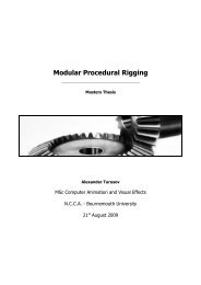
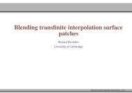
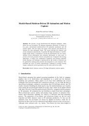
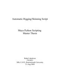
Figure 1: Separate user dened elds combined into a nal velocity eld, createdby Rhythm and Hues using FELT. Image taken from [6]also limited in terms of control. These solvers will provide good results quickly,but are not able to be extended or internally modied by users for more specicrequirements.3.2 Proprietary Systems3.2.1 Rhythm and Hues' Field Expression Language ToolkitAn example of a proprietary system that helps dene 3d scalar and vector eldsis a tool developed by Rhythm and Hues. They create and combine user denedvector elds using FELT, their Field Expression Language Toolkit as can beseen in Figure 1. The resulting velocity eld is used to drive particles for themovie The Incredible Hulk [6].3.2.2 ILM's directable, high resolution reILM has created high detailed re for the movie Harry Potter and The HalfBlood Prince, using particles that were rst advected by a low resolution uidsimulation and then were used to ll up eld information such as temperature,velocity for high resolution 2d elds [10]. Those elds are then processed bya uid solver solving velocity, density and temperature. The particles are projectedon 2d slices perpendicular to the camera, similar to the way sprites facethe camera as can be seen in Figure 2. Because the slices are 2d, the resolu-4

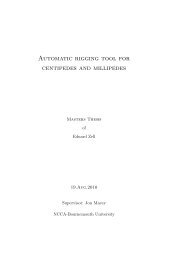
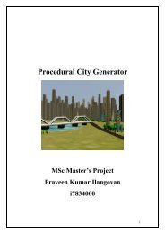
Figure 2: High resolution 2d uid containers controlled by information fromprojected particles created by ILM. Image taken from [10]Figure 3: Advecting the simulation with curl noise where turbulent energy isdetected. Image taken from [14]tion can be raised quite high. The interesting part is that the relatively smallamount of particles are used as a way to dene the high resolution elds. Theparticles represent a custom eld, this hints towards the idea that the customeld does not need to have a very high resolution as some of the simulationsonly used 20.000 to 100.000 particles.3.3 Research3.3.1 Introducing noise in the velocity eldAnother example of the use of a custom eld to give more interesting resultsin uid simulation is the introduction of curl-noise for procedural uid ow [3].They generate turbulent velocity elds based on Perlin noise. This type of noiseis procedural but could just as well be added to uid simulations, which is whatis being done in [14] with the additional condition that the curl noise is notadvecting the velocity everywhere, but only where their physically motivatedenergy model dictates it as can be seen in Figure 3.5

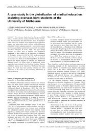
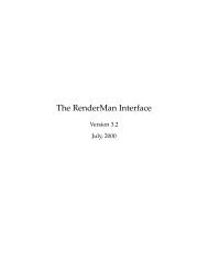
Figure 4: The dierent states of target driven smoke using custom elds. Imagetaken from [7]3.3.2 Target driven smoke animationCustom elds can also be used to create target driven smoke animations, as in[7]. They introduce a driving force term that causes the uid to carry the smoketowards a particular target and they also add a smoke gathering term whichprevents the smoke from diusing too much due to numerical dissipation. Thecore concept behind this technique is using the gradient of a blurred densityeld of a target shape as direction vectors to advect the velocity eld of thesmoke. The resulting vector eld looks like all the vectors are pointing towardsthe target shape. Because the start and end shape might have dierent densitiesor the smoke might lose density along the way, density is added as it interpolatesbetween the two shapes as can be seen in Figure 4.3.4 A broader publicThe above approaches use custom elds and geometry to gain more controlover the simulation, but they are separate or proprietary software solutions.Because they are custom built they have the advantage that they will t withinthe pipeline of a particular company and are able to explore new hardwareplatforms such as the GPU. The drawback is that these tools are not veryportable and useable by a broader public.3.4.1 Node based dynamic simulationsOne company that is trying to change the way uid simulations are set upis Exotic Matter with their software called Naiad [5]. The creators are MarcusNordenstam and Robert Bridson who have both contributed greatly to thedevelopment of uid solvers over the past ten years. Robert Bridson has publishedseveral insightful papers and also the book Fluid Dynamics for ComputerGraphics [2]. At its core Naiad is a dynamics solver and a simulation framework.Naiad allows for the creation of a description of a simulation scene. Thisdescription can then be simulated. The description can be made through a nodebased interface which resembles that of node based compositing software as can6

Figure 5: The node based operator graph in Naiad, by Exotic Matter. Imagetaken from [5]be seen in Figure 5. They are trying to establish a Nip (Naiad Interface Protocol)format which is similar to a RenderMan RIB format, but then for dynamicsimulation. This has not been done before and will hopefully help establish astandard for dynamic simulations. This is also one of the few systems whichuses a node based approach for uid dynamics, the other major node baseddynamics system is part of Houdini.3.4.2 A brief history of Houdini's dynamic contextSince Houdini 8 node based dynamic operators (DOPS) were introduced andsince Houdini 9 uids and gas microsolvers were added. Houdini 10 brought afurther development of a preset pyrosolver which can produce high quality pyrotechnicresults combined with an extensive pyroshader. They also introduced7

Figure 6: The various microsolvers available in Houdini's dynamics context.an upres technique which greatly increases the detail in the nal high resolutionresult. To handle these high resolution simulations they allow distributedsimulation over a network of computers. These developments and techniqueswill be explained in greater detail in the next section as they are important tounderstand the proposed workow and tool.4 Technical BackgroundHoudini's node based architecture is open and not a black box. For example thepreset pyrosolver is a digital asset, which means it can be unlocked, modiedto support extra functionality and saved as a new custom solver. ThereforeHoudini is very well suited to get more control over uid simulations. Howeverin order to determine where to insert extra functionality and make modicationsan explanation of some of the current uid techniques and their implementationin Houdini is required. Some of the equations of uids will be explained forcompleteness and some of the equivalent microsolver networks will be shownalongside.4.1 What are microsolvers?Microsolvers are nodes inside of DOPS that perform specic tasks related tothe uid solving process. Instead of solving various aspects of a uid simulationin one big solver node as is done with the preset smoke- or pyrosolver, amicrosolver performs only a specic mathematical task. By wiring these microsolverstogether more complex operations can be performed, this is how thebigger smoke and pyro solvers were created. Some microsolvers are digital as-8

sets, which means they are built from a network of smaller microsolvers inside.There are currently around 60 microsolvers in Houdini 10 as can be seen inFigure (6). It is beyond the scope of this thesis to cover all of them so instead afew of the more important ones of which the equivalent often shows up in uidequations will be covered. Microsolvers are wired together by using a mergedop, the order of the inputs is very important as it will dene which microsolvercontributes to the nal result rst. The order of operations works from left toright, top to bottom. This is quite dierent from the pure top to bottom nodeow inside of the surface operators context (SOPS).4.2 How do volume elds work in Houdini?4.2.1 Dening scalar and vector eldsVolume elds in Houdini come in two types: scalar elds and vector elds. Theyare dened as primitives in SOPS (surface operators) but can also be createdin DOPS (dynamic operators) and represent an attribute of the volume, themost commonly known is the density scalar eld. Other custom elds can bedened using a volume sop which will dene an empty volume primitive or aniso-oset sop which will dene a volume based on the closed mesh of an inputgeometry. One of the more powerful ways to dene custom volumes is by usingthe volumevop. This runs CVEX (Houdini's vertex expression language) overa set of volume primitives, the operations can be dened through code or bybuilding a CVEX VOP (vertex operators) network. Not only do you have a lotof low level mathematical functionality, using VOPS will compile the resultingnetwork in vex code which will make it a lot faster to run in comparison tonormal expressions which would have to be interpreted. This volumevop is usedas part of the tool that was developed to dene custom elds in SOPS.In DOPS elds can be created using a (SOP) Scalar Field node or a (SOP)Vector Field node. The (SOP) part allows you to reference elds from SOPS,but sometimes temporary elds are needed to store results of calculations andthe eld is created without the need to reference it from SOPS as it will be lledup with data that is calculated from other elds in DOPS. To quickly create anempty eld based upon the properties such as the dimensions and resolution ofanother eld, a Gas Match Field microsolver can be used.A scalar volume eld such as density will contain a single primitive, whereasa vector eld such as velocity will contain 3 primitives, one for each component.By convention the velocity eld is named vel, the components are vel.x, vel.yand vel.z.4.2.2 Naming volume primitivesIt is important to give the correct names to scalar elds before merging theminto a single vector eld. Some elds are recognised by the preset shaders, suchas the color eld (Cd), but are not yet supported by the preset uid solvers.By modifying the preset shaders you can have custom elds inuence the look9

and create extra output variables that can be rendered to separate image planesfor greater control in a compositing application. Another useful eld to haveas part of the simulation is the rest eld, which basically carries a set of uvcoordinates that can be used to map textures to the uid.Fields can be given any name, but only certain specic elds will be pickedup by the Mantra render engine, for example if the vel eld is detected andmotion blur for rendering is turned on, the information of the velocity eld willbe used to apply motion blur on a fast moving uid simulation.4.2.3 Rest eld interpolationIn the preset smoke solver a single rest eld is advected along with the otherelds. This rest eld is then used inside a volume shader to map various kindof noise to the uids and increase the detail of the smoke as is also describedin [17]. When this rest eld is advected far away from the initial position, thetextures will become distorted which can give undesirable results. In the newpyrosolver in Houdini 10 a second rest eld (rest2) is introduced to solve thisissue. The initialization of both elds (rest and rest2) is staggered in time andthe pyro shader continually interpolates between them. For example if the resetvalue on the pyrosolver is set to 50, the rest eld will be re-initialized every50 frames, starting at the rst frame. The rest2 eld will also be re-initializedevery 50 frames, but will start at frame 25 (half of the reset value). The pyroshader has a corresponding Reset Rate parameter that should be set to thesame value. This will cause the shader to interpolate between the two rest eldswithout showing any popping when the rest elds are reinitialized.r e s t : +−−−−−−−−−−−−−+−−−−−−−−−−−−−−−+−−−−−−−−−−−−−−− ( e t c )r e s t 2 : −−−−−−+−−−−−−−−−−−−−−−+−−−−−−−−−−−−−−−+−−−−−−− ( e t c )At each + in that graphic, the eld resets. The pyro shader then constantlycross-fades between the two elds, such that a given eld has full contributiononly at the reset frame [12].4.2.4 Volume eld viewport visualizationWithin DOPS there are dierent way to visualize the information stored ina eld. This visualization can greatly help to visually debug the values of aeld. To be able to enable this visualization for a specic eld, a Scalar/VectorField Visualization node needs to be attached to the data input of a eld. Thisvisualization can consist of:• showing the eld as smoke (useful for density),• as straight lines depicting both length and direction of the values of avector eld (generally useful for a static or dynamic velocity eld),• as streamers, which are curves depicting the ow of a vector eld, (usefulfor viewing the interpolation of the velocity between voxels)10

• as an axis aligned plane that shows a coloured slice in the volume, mappingthe values of the eld to the colours on the plane. (useful for temperature)Within SOPS a volume will generally be visualized as smoke when the values ofthe eld are positive. This means as well that when you are trying to visualizea eld that has negative values, such as velocity or temperature, nothing willbe shown in the viewport in SOPS, even though the data is actually there. Aquick check can be performed by taking the absolute value of the data insidea volumevop just for visualization purposes to make sure the data exists. Atthis point visualizing your custom elds in dops will give you more options asdescribed above. The reason why this section on visualizing volumes in SOPS isincluded is because it is not in DOPS, which means no solving needs to happento visualize the eld which makes it faster to shape volume elds independentof the previous frames. Also it is important to understand negative values arenot displayed in the viewport as this clarication will hopefully avoid confusionlater on when the tool is used and there seems to be no output.4.2.5 Houdini specic trainingSidefx, the creators of Houdini, provide a great set of masterclass tutorials onuids and the pyrotools on their website which will help when learning how touse microsolvers and understand volume elds in Houdini [15].4.3 The equations of uidsA signicant amount of research has already been done in the area of computationaluid dynamics (CFD) for simulating smoke, re or various types ofliquids. A few of the equations will be covered to help explain the componentsthat make up a simple smoke solver in Houdini.4.3.1 The incompressible Navier Stokes equationsThere is a consensus among scientists that the Navier Stokes equations are avery good model for uid ow [17]. That is why they tend to be used as afoundation for a lot of solvers, that will then in some way modify or extendthese equations:∂⃗u∂t + ⃗u · ∇⃗u + 1 ∇ρ = ⃗g + v∇ · ∇⃗u (1)ρWhere:⃗utρgvvelocitytimepressurebody forcesviscosity∇ · −→ u = 0 (2)11

And (1) is called the momentum equation and tells us how the uid acceleratesdue to the forces acting on it and can be derived from Newton's equation−→ F = m−→ a as explained in [4]. And (2) is the incompressibility condition andstates that the divergence of the velocity must always be equal to zero. Thisconstraint ensures that the sum of all velocities entering and leaving at a pointin space is zero. When this is conserved, the total mass is conserved over theentire simulation [18].4.3.2 The steps to solve the Navier Stokes equationsThree main steps will be required to solve the Navier Stokes equations, thesesteps are very well described in [18] but will be included here again for completenessand some of the explanations of the terms summarized.1. Advection2. Diusion and External forces (Body forces)3. pressure/incompressibilityAdvection( −→ u · ∇) −→ uAdvection represents the fact that the motion of the uid causes motionof the entities within it. This can be thought of as the velocity of the uidmoving itself along, and is sometimes referred to as self-advection because ofthat property. The advection part of the equations can also be used to modelmotion of other entities inside the uid [18].Within Houdini the Gas Advect microsolver can be used for advecting one orseveral elds at the same time. For more advanced interactions between elds,other actions can be performed at this step that will update the elds. This canbe seen in the node tree for the elds_updates section inside the preset smokesolver in Figure (7). For instance:• A Gas Blur is used to diuse the temperature eld,• A Gas Calculate is used to cool the temperature eld or to copy informationfrom a source eld into a heat eld.• Fields are not the only thing that can be advected, geometry can as well,such as vorticle geometry which is explained in the external forces step.Diusion and External forces12

Figure 7: The node tree for the update elds section in the preset smoke solverin Houdini as described in (4.3.2)13

Diusionv∇ · ∇⃗uThe diusion allows the velocity to propagate outwards from its currentlocation, with the viscosity parameter controlling how fast this happens. Highviscosity yields thick and slow uids while, while a low viscosity yields livelyuids [18].Within Houdini the viscosity can be implemented using a Gas Diuse microsolver.This outwards going velocity is a modication to the velocity eld.External forces⃗gThis is considered as the sum of all external forces. Some typical forcesare wind, drag or gravity, but also include more advanced forces that requireseparate simulations, such as the forces generated by temperature dierences.These external forces can be extended and provide a lot more control by addinguser dened volumetric elds. This is one of the areas that will be extended withcustom elds dening them in SOPS with the custom tool that is developed.Within Houdini these forces can be represented by a variety of Gas Microsolvers,that create the total resulting force when merged together. Typicalmicrosolvers that are part of the preset smoke solver for the forces componentare the following and can be seen in the node tree of the forces section of thepreset smoke solver in Figure (8):• Gas Vortex Connement: to re-introduce some of the lost velocity due tonumerical dissipation, a high vortex connement force will introduces alot of swirling motion in the simulation,• Gas External Forces: both for external forces relative to density or absolute.When relative it will scale the velocity by another eld, maskedby the density, when absolute it will simply scale the velocity by anothereld without the mask,• Gas Buoyancy: to calculate an approximate buoyancy force dependent ona temperature eld,• Gas Diuse: for the viscosity force, as explained in the diusion stepabove,• Gas Vorticle Forces: for introducing extra swirling motion around eachvorticle, according to the vorticle attributes. By default when addingvorticles, the vorticles are particles that exist throughout the entire volumeand that are advected by the velocity,• Gas Calculate: for setting minimum and maximum speed limits if required.14

Figure 8: The node tree showing the body forces inside the preset smoke solverin Houdini as discussed in (4.3.2)Pressure and Incompressibility (non-divergence)PressurepThe pressure can be considered as the uid from the area with high pressurethat will be pushed by the pressure towards the area with lower pressure. Thisforce is represented by the gradient of the pressure eld, p [18].The incompressibility condition∇ · −→ u = 0Another way to think about pressure is that it is whatever it takes to keepthe velocity divergence-free so the incompressibility condition is satised [4].Within Houdini these terms come in the shape of a Gas Project Non Divergentmicrosolver that removes any divergent portions of a velocity eld. Theseare parts of the velocity eld that represent expansion or contraction. Thisis done by computing a pressure eld that counteracts any compression andapplying that pressure eld instantaneously [16].4.3.3 Vorticity ConnementWhen simulations of stable uids are run, some of the velocity is lost due tonumerical dissipation which is the results of a necessary weighted averaging step15

during the advection term. It has the eect of unintentionally adding viscousbehavior to the uid, which can damp down some of the intricate turbulentbehavior seen in natural smoke and re[13]. In [8] a method is described fordetecting the vorticity and adding the rotational forces back in. Each smallpiece of vorticity can be thought of as a paddle wheel trying to spin the oweld in a particular direction. Articial numerical dissipation damps out theeect of these paddle wheels and the key idea is to simply add it back.The vorticity connement calculation is a good example in Houdini of howsome of the microsolvers and elds can be used together. A Vortex Connementmicrosolver exists, but it is really a digital asset made out of smallermicrosolvers.These are the steps that are executed within the Vortex Connement microsolverand the accompanying node tree can be seen in Figure (9):1. Create the elds for temporary results: curl (vector), curl magnitude(scalar) and vortex direction (vector) using Gas Match Field microsolvers.2. Calculate the curl of the velocity eld with a Gas Analysis microsolverand store the result in the curl eld.3. Calculate the length of the curl eld and store it in the curl magnitudeeld using a Gas Analysis microsolver.4. Calculate the gradient of the curl magnitude eld and store it in the vortexdirection eld using a Gas Analysis microsolver.5. Normalize the vortex direction eld using a Gas Analysis microsolver.6. Calculate the cross product between the vortex direction eld and the curleld with a Gas Cross microsolver and store the result back in the vortexdirection eld.7. Multiply the vortex direction eld by a scalar to increase the amount ofconnement using a Gas Calculate microsolver.8. Multiply the vortex direction eld by a connement eld to increase theamount of connement only at specic location within the eld using aGas Calculate.9. Update the velocity by adding the vortex direction eld to it using a GasCalculate microsolver.10. Clear the temporary elds by copying 0 into them using a Gas Calculatemicrosolver.From the above steps it becomes clear that the Gas Calculate, the Gas Analysisand the Gas Match Field are very useful microsolvers, and will come back allthe time. They are some of the mathematical building blocks to build morecomplex operations. While developing these operations the visualization of theresulting steps can be very helpful as shown in Figure (10).16

Figure 9: The node tree in Houdini for the Vortex Connement microsolvershowing all the steps as described in (4.3.3)17

Figure 10: The geometric representation of the steps inside the Vortex Connementmicrosolver as described in (4.3.3). Red represents the curl eld after step2, green represents the gradient of the curl magnitude eld after step 5, bluerepresents the vortex direction after step 8.18

4.4 Up Res techniqueIn Houdini 10 a new technique was introduced were a low resolution simulationcan be used as the basis for a higher resolution simulation. The key conceptis that you get the general motion from the lower resolution simulation andintroduce high frequency noise into the velocity eld, but only where there isa high curvature. The introduced noise has a low amplitude so it does notinterfere with the general motion coming from the low resolution velocity eld.A cut down version of the pyrosolver is used for the Up Res phase as a lot of theinformation is coming from the low res elds rather than having to be calculatedfrom scratch. Because it is still a high resolution simulation it can take a longtime. The foundations for this Up Res technique were initially built in Houdini9.5 based on [11]. It then became a fully integrated tool supporting Constant,Wavelets and Curl noise. The Gas Up Res solver is also a digital asset, whichmeans it can be modied to support custom user dened elds coming from thelow res simulation or added in to support a certain type of control or new typeof noise. Those elds can then be up-ressed and written to disk at the end ofeach simulation step.4.5 Distributed simulationsRunning high resolution simulations can take a lot of time. Therefore the functionalityhas been built in to be able to split a heavy uid container into slices.These slices represent partitions of the volume. The amount of overlap betweenthe slices that is required for a good distributed simulation depends on the speedof the uid and needs to be set by the user. There are several ways the slicescan be dened, but by default they will partition the space inside the containersimilarly to a binary tree. Each slice can then be calculated on a dierentmachine that is connected to a host machine that is running a tracker. Themachines share the data between them in the overlapping regions through interprocess communication. The speed gains are signicant, but not linear as theextra overlap and communication between machines takes up a bit of additionalprocessing power. The simulation generally runs as fast as the slowest machine.If all the machines have the same specications this is not a problem, but if oneof them is signicantly slower than the others, the faster machines will not beused as eciently.Sidefx has provided Hqueue, a python based renderfarm software to helpwith this distribution. However HQueue was not tested for this project due tolimited administrative permissions. Instead a few shell scripts were written thatremotely start a tracker and the simulations and make use of the exact samedistribution techniques. Again it is convenient that open access is provided tothe distribution techniques without forcing users to use HQueue.19

5 A workow for using and creating custom volumeelds in Houdini.5.1 IntroductionThe aim of this project was to get more and better control over uid simulationsusing custom elds. To be able to have this kind of control the problem isapproached from two sides. The rst side is by dening custom elds inside ofSOPS, the second side is by using microsolvers to integrate those custom eldswith existing solvers and perform certain mathematical calculations to solve therequired needs inside of DOPS.These custom elds are dened in SOPS and brought into DOPS. In orderfor them to work correctly they need to be inserted in a uid solver at theright place, some of this has been covered in section (4). Custom elds canadd any kind of data to the simulation. For example: add color, temperature,velocity, fuel, density, etc. Some of these attributes are already supported by thepreset solvers and can be easily modied. Others will need extra implementationthrough the use of microsolvers. There has already been done a lot of work in theeld of computational uid dynamics and some of the preset solvers in Houdinicover a lot of this functionality. The aim of this project is not to create a fulluid solver with a combustion model from the ground up, but rather to be ableto modify and augment existing solvers.By controlling the uid simulation through custom elds, depending on whatexactly is modied, some of the physical accurateness of the simulation will belost, but that is the whole point as by introducing custom elds (art-)directablesimulations are possible. The goal of this project is not to build a physicalsimulator, but rather to understand a physical simulator and then insert extraelds into it to augment the possibilities of the solver. Ideally the uid ow andturbulent behaviour is maintained within the modications, but if certain eldswill be overwriting other elds because this provides better visual results thenthis is considered an improvement.5.2 The implementation of an attribute transfer tool inSOPS to help dene custom volume elds.There are a few microsolvers inside DOPS that will allow to bring data fromSOPS into DOPS already:• The Sop Scalar/Vector eld microsolver which can bring in a fog volumethat has been dened in SOPS through an iso-oset sop.• The Gas Particle To Field microsolver allows point attributes from particlesto be copied into a eld, after the particle geometry has been denedinside a SOP Geometry dop. This microsolver allows for most of the requiredfunctionality, but it is in dops which requires the simulation to cookup to the current frame as soon as a change is made.20

• The nal option is with a Gas Field Vop which provides all the functionalityfrom vops so you can reference in any object from a dierent context,or from a le on disk.In SOPS however this attribute transfer from points to volumes does not existand is a welcome addition as it does not have the requirement to simulate all theprevious frames to dene the eld. Also the resulting custom volume elds caneasily be used to advect particles inside of a pop network by using an Advect ByVolumes pop without even going near DOPS. The reason that this just works isbecause the tool follows the standards used by Houdini to dene volume eldsas described in (4.2).5.2.1 A pointcloud based approachThe rst approach to transferring point attributes from a number of pointsmakes use of pointcloud functionality inside of a volumevop in sops. The underlyingtechnicalities are hidden away behind an easy to use interface. I deliberatelykept this digital asset compact as it needed to perform only a singlefunction. The rst input requires an empty volume, the second input requires atits lowest level a number of points. The volume eld name can be specied, aswell as the attribute to transfer and the attribute type. The attribute type willalso dene the type of volume that is created (either a scalar or vector eld).The distance threshold denes how big the inuence radius of each point is. Inthe pcloud tab a maximum search radius is provided to prevent voxels lookingup values from points outside this radius. Also the maximum number of pointsto use when performing the ltering operation can be set here. Generally thedefault values work for most scenarios.Internally the asset creates a box that matches the position and divisions ofthe voxel grid. Then an attribute transfer sop is used to transfer the attribute tothe grid of points. The grid is used instead of using the points directly becausethe attribute transfer sop uses a metaball kernel inside to dene the fallo ofthe attributes and give softer results around the edges of a shape. These pointsare then referenced by a volume vop which will read them as if they were apointcloud from disk. For each voxel it will then lter the attribute value andassign it to the output density. The output density is just a name inside thevolume vop, it could just as well be the x component of a velocity eld. The realnaming of the volume occurs before or after the volume vop assigns the valuesto the eld. In case of a vector eld and a vector attribute each individualcomponent is handled at a time and then the resulting scalar elds are mergedtogether to form the resulting vector eld.This gives quite accurate results, but can get slow for high resolution volumes,as the attribute transfer sop can take a while to cook. Bypassing theattribute transfer and using the points directly will denitely speed it up, butdoes not give as nice results, this bypass is triggered by turning on the Use RawPoints checkbox on the digital asset interface in the pcloud tab. Also this approachdoes not allow a way to dene a transfer radius per point, only a globalradius can be used.21

Figure 11: The parameters of the metaball-based volume attribute transfer tool.5.2.2 A metaloop based approachThe original way of dening volumes through metaballs involves copying metaballsonto the points, converting them to a fog volume using an iso-oset withthe Mode set to Meta Balls. The problem is that this only uses the density ofthe metaballs and none of the potential other attributes.The volume attribute transfer tool is based upon this workow but againmakes use of vops functionality to perform the lookup of the attributes manually.Similar controls are provides as with the pointcloud approach, althoughthis tool was further developed and presets were added to make it easy for usersto transfer popular attributes that can be used from a drop down menu. Theinterface of the tool can be seen in Figure (11). This tool also allows the possibilityto dene a per point transfer radius by using the pscale attribute if it ispresent on the template geometry.Inside of the digital asset, expressions are used to help dene the presetsettings. Metaballs are copied onto the template points and are then referencedby a volumevop. Inside of the volumevop a while loop is created that will loopthrough all the metaballs, lookup the value of each one at a given position andadd the result together. This is the default density calculation. When trying toadd a dierent attribute together the results were very blocky, the reason whythis was happening was because the attribute would be dened as a solid box ofa constant value within the bounding box of a metaball. This is a problem verysimilar to 2d sprites that have not had there alpha channel premultiplied. Sothe solution was to multiply the attribute with the density value of the metaball,this problem is represented in Figure (12). The density needs to be multipliedinside the deepest level of the metaloop, just before the attribute is added to theresult of the previous metaball, not as a post multiplication operation becausein overlapping areas the masking will be incorrect, the post multiplication eect22

Figure 12: Premultiplication problems: The image on the left shows the attributein grey and the density of the metaball in white.The image on the rightshows the correct premultiplied values.is shown in Figure (13), the artifacts are not that visible in a still frame but willcause jittering during animation.At this point the values are simply added together, which works well fordensity, but not so well for velocity or color. For example in the case of particlesbeing emitted from a single point in space and then spreading out from thatpoint over time, what would happen is the density would be accumulated andlook good, but because of the dense number of particles at that single point, thevelocity eld would grow extremely large and when this entire resulting volumeis then rendered by mantra with motion blur turned on, huge streaks are createddue to the high velocity accumulation.So more control was needed to dene the kind of mathematical calculationthat takes place. Therefore an averaging operation and a switch is added, so theuser can choose whether to accumulate the values or to average them. This is nottrivial and this choice should be provided to the user. A temperature eld forinstance might require either accumulation or averaging, both could work andwill give dierent results. The presets try to alleviate this issue for some of thepopular attributes based upon what works better for those attributes in mostscenarios so the user does not need to worry too much about this. However ifthe accumulation of velocity attribute were required, the user can set the presetto other and dene v as the attribute, vector as the type and add as theblend operation as the other preset allows any custom attribute to be used.Because the copy sop inside of the asset transfers the template point attributes,the special attribute pscale can be used. When a pscale attribute isdened on the template points, the metaballs will be scaled based on the pscalevalue. This tends to give good results, however when the pscale goes to zero,jittering in the volume might occur if the points are moving. It would be as ifthe small metaball would only occasionally be picked up by a voxel when it is inclose enough proximity. A better way of dealing with this problem is by usingthe weight attribute instead of the pscale. This will not modify the radius, butwill instead result in more of a fading eect. The best results can be achievedwhen both are used together.23

Figure 13: Incorrectly post-multiplying of the attribute (temperature) by thedensity will cause artifacts, note the banding in the brighter areas, that becomemore apparent in an animation.24

Figure 14: The preset smoke solver with the color eld added to it, as describedin (5.3.1)5.3 Examples of custom eldsThe next sections will talk about how some setups can be created and what isrequired to implement the custom elds in dops for each example.5.3.1 Colour eld additionOnce the colour (Cd) attribute is transferred onto a volume in SOPS using thevolume attribute transfer tool, the necessary elds can be added in DOPS, thenode tree can be seen in Figure (14) :1. A Sop Vector Field, Cd, is dened to bring in the newly dened Cd eldfrom SOPS. This eld will contain the color information throughout thesimulation.2. Another Sop Vector Field, Cd_source, is dened using the Cd eld fromSOPS. This eld will be used to add color information to the Cd eld atthe beginning of every frame. If this eld is animated, it is required thatthe Time and SOP Path are always evaluated. The Time parametershould be set to $T.3. Using a Gas Calculate with a the calculation set to Maximum, the destinationeld set to Cd and the source eld set to Cd_source will copyinformation from the source into the destination eld at the start of everyframe using a maximum operation.4. Advect the color eld by the velocity, using a Gas Advect microsolvers25

Figure 15: Two spheres emitting density and color with a vortex force applied.5. Diuse the color eld using a Gas Diuse microsolver, the diusion rateshould match the density diusion rate. For fast mixing of the color, thisvalue can be increased.In Figure (15) two spheres can be seen emitting density and color informationinto a simulation. This simulation has the color elds dened as copies of thedensity values for either the red or the blue component of the Cd vector eldand does not actually require the transfer tool in SOPS. In Figure (16) you cansee a helix curve emitting density, colour and the temperature eld is driven bythe red values of the colour which causes the red smoke to rise quicker. The hueof the colour is mapped to the parametric u value of the curve.5.3.2 Advect by curveIn this example the tangent vectors of a curve are used as an extra force thatis continuously added to the velocity eld. A relatively large amount of force isapplied. Also the density eld is temporarely blurred, the gradient is taken fromthis blurred density, then normalized and applied as an additional force. Thecombined force points towards the density of the curve and along the tangentof the curve. A sphere is placed at the bottom of the helix and is emittingdensity into the simulation. The density and tangent velocity elds can be seenin Figure (17).The node tree can be seen in Figure (18) and consists of the main followingareas:26

Figure 16: A helix curve emitting density, colour and temperature into thesimulation. The red component of the colour is driving the temperature, thatis why the red smoke is rising quicker.Figure 17: The density eld and tangent velocity eld dened by a helix curveand used to advect smoke.27

Figure 18: The node tree for the dierent steps for the advect by curve simulationas described in (5.3.2).1. Dene a few custom sop vector elds to hold to custom dened volumesfrom sops, such as the density source (the little sphere), the custom densityof the curve, the tangent velocity and the gradient velocity (which will becalculated at a later step).2. Calculate noise by dening new custom elds with the Gas Match Fieldmicrosolver, a scalar noise_eld and a vector noise_vel eld and denethe noise in the noise_eld inside of a Gas Field Vop using an Anti-Aliased Flow Noise vop. By using a Gas Analysis microsolver we cancalculate the gradient of the noise_eld and store it in the noise_vel.3. Calculate the gradient of the blurred density of the curve. Create a newtemporary eld to store the blurred_custom_density using a Gas MatchField, matching the custom density eld of the curve. Copy the custom_densityinto the blur_custom_density using a Gas Calculate. Blurthe blur_custom_density eld using a Gas Blur. Calculate the gradientof the blur_custom_density and store the result in the gradient_velocity.Finally normalize the gradient_vel using a Gas Analysis. The resultantforce will appear to be always pointing towards the helix shape.4. Add the forces to density. By using Gas Calculate nodes, the variouscustom velocity elds can be premultiplied by higher values for a morepowerful eect and added to the velocity eld.The simulation can get unstable when too much force is added, so it can beuseful to add a low velocity damp on the pyrosolver, or even turn on speedlimits.A few stages of the simulation can be seen in Figure (19).28

Figure 19: A few stages of the advection by curve. These images were ipbookedfrom the viewport.5.3.3 Custom fuel and heat injectionThe following examples all make use of the combustion model inside the pyrosolver.By providing fuel and adding temperature, smoke and ames can begenerated from the resulting density and heat elds. Some of these simulationswill have vorticle geometry in them to add more turbulent motion.Fuel from curve In this example the helix curve was used to dene an initialfuel eld inside of the pyro object. A fuel eld is a default eld and does notneed a custom eld unless you want to have an animated fuel eld, for thisexample however the fuel eld is static. Only one custom eld is added to addtemperature to the bottom part of the fuel eld. The buoyancy direction on thepyrosolver is set to a negative y direction to avoid the heat from rising throughthe helix and igniting other parts before it is supposed to get there even thoughthat is visually quite interesting as well. The only step during the advectionprocess that is added is to add temperature from the custom source temperatureeld to the temperature eld that will then be used by the combustion modeland start the ignition. The burn rate on the pyrosolver is set to 2, so it burnsquite fast and the temperature output is set to 6, so a lot of heat is generatedwhich will keep the simulation going. The dierent elds at dierent stages canbe seen in Figure (20).Fuel from animated geometry In this example an animated model of atree is used as a source geometry to dene animated volumes of both fuel andtemperature. The animated model was provided by Nick Hampshire, who createdthe animation through a real-time spring solver that he programmed forhis Master thesis [9]. As the geometry represents a moving point cloud at itslowest level it works will with the attribute transfer tool. The fuel eld hasthe appearance of spreading out through the branches which was achieved bycopying an animated attribute from a static mesh of the tree to the animatedmesh of the tree. The attribute simply spreads in a radial fashion, although itwill spread faster at the outer points of the branches and slower at the root of29

Figure 20: The purple eld represents the fuel, the yellow eld is the burn andthe white eld is the density resulting from the combustion in the fuel fromcurve example.the tree where the branches are thicker, the animated geometry with the spreadingattribute is then baked to disk to speed up the rest of the network. Thisattribute is then transferred using the volume transfer tool. The temperatureeld is the same as the fuel eld. The tree geometry came with point velocitieson it but those could alternatively be calculated with a trail sop as the topologydoes not change over time. These velocities are also transferred into a customeld.In DOPS those three custom elds are brought in with Sop Scalar/Vectorelds and their SOP path and Time ($T) parameters are set to Always evaluate.During the simulation step the elds are added to their respective target eldsusing Gas Calculate microsolvers. The fuel eld is not added with a maximumoperation as this added too much fuel into the simulation which resulted in amassive explosive reaction, so instead it is copied every frame and overwritesthe old fuel data from the previous frame. A Gas Dissipate is also added toslowly dissipate the density. The various stages can be seen in Figure (21).Fuel from particles In this example a simple terrain is modeled and particlesfall down from above the terrain and collide with it. A particle that is collidingis added to a collision group. Outside of the particle network in sops, the pointsthat are not in the collision group are deleted. The amount of collisions caneasily be increased or decreased depending on the birthrate parameter of thesource pop inside the pop network. At each frame there are generally betweenone and three particles in the collision group. By using an attribute transfer,the normal from the collision surface is transferred to the particle. Now thevolume attribute transfer tool is used to dene the fuel and temperature eldsbased upon the metaball density. A custom velocity eld will also be generatedwith the tool, using the normal attribute from the particles which has just beentransferred from the surface.30

Figure 21: Top: The stages of the animated fuel eld, Bottom: The stages ofthe rendered burning tree.In DOPS the setup is very similar to the fuel from animated geometrysetup. Because fuel, temperature and velocity are only added where the particlesare currently colliding and a low number of particles is colliding per frame,not too much fuel is added each frame. Therefore in the Gas Calculate themaximum between the custom_fuel_source and the fuel is calculated. Thecustom_fuel_source eld is premultiplied by a factor of 5 to introduce morefuel into the simulation. The transferred custom_velocity_source is heavilypremultiplied by a factor of 150 before being added to the velocity eld. Sincethe velocity direction is coming from the surface, the explosions are not directedstraight at the sky. On the pyrosolver the ineciency in the combustion modelis set to 0.6 which causes some of the fuel to not be fully burnt. The burn rateis set to 0.8 which will cause the fuel to take longer to be consumed. This cangive good results combined with the initial velocity as the burning fuel will beadvected by the velocity and will continue to be burn as it is lifted up into thesky. A small amount of velocity damp is also introduced so the velocity wearso after the initial boost. The dierent elds can be seen in Figure (22).6 ConclusionThe control Houdini oers over manipulating dynamics and performing moreadvanced mathematical calculations is extensive and there are many more microsolversto study. Also uid dynamics for computer graphics is a populartopic of research and new developments are happening all the time. A signicantamount of time for this project went into researching existing ideas in uidsfor computer graphics and in how volume elds and the microsolvers work togetherin Houdini. Gaining a complete understanding of how the preset smoke31

Figure 22: Fuel, temperature and velocity are transferred from colliding particlesand set o small explosions. The fuel is purple, the heat is yellow, and thedensity is white. The initial velocity upon collision is shown as the big red lines.32

and pyrosolver work took time. This research only started to become more applicablehalf way through the project as various experiments were developed. Alot more experiments can be done, especially by modifying the velocity eld, butit seemed more valuable to focus on a wider range of dierent types of customeld implementations to show a broad use of the tool and the possibilities byusing custom elds. The aim was to gain control over uids by using customelds and this has been achieved through the prototype experiments. Theseexperiments are by no means production ready, as higher resolution simulationscould have given much more detailed results. But that would also have taken alot more time.The main strength of this project is that the tool that was built is easy touse with a variety of applications, yet enables users to use all the functionalityof sops, from creating geometry such as curves or particles to dening specicanimated point attributes through expressions or vops to create those artisticvolume elds. And because the tool follows conventions for dening volumeelds, the elds can be used in other context besides dops, like pops or forrendering with Mantra. Within the metaball tool there is still an optimizationthat could be made when dealing with vector elds, because the volume vopis used separately for each component and ideally would only be used once forall the components in one go. This would speed up the tool signicantly asthe metaball loop only needs to be executed once instead of three times. Theproblem lies with the output of the volume vop in SOPS, which seems to allowonly a single scalar eld to be exported and what is needed is a vector eldexport option.The microsolvers within Houdini are powerful mathematical building blocksthat are able to build bigger structures like vortex connement or entire solvers,however since the author was quite new to the eld of uid dynamics a goodunderstanding and knowledge base needed to be built up rst before more interestingexperiments could be set up. By following the mathematical equationsalongside the microsolver networks and being able to visualize the outcome ofa given calculation in the viewport so it would make sense on a geometric level,the author was able to get a good understanding of uid solvers and how tomodify them. The author recommends learning Houdini uids this way as youget information from both sides. Overall this project has been an interestingexperience even though it was biased more towards the research side than theproduction side than was originally planned. By putting the equations next tothe microsolver node networks the author hopes to have been able to create abetter understanding for other Houdini users or perhaps opened up the doorfor researchers who would want to use Houdini for development of uid solvers.By not focusing on the implementation of one big digital asset performing onespecic eect, but instead building a small and comparatively light, very usefulbuilding block to help dene custom elds, a much broader application of thetool is possible. The tool is like a microsolver in SOPS.33

ThanksThanks to Coen Klosters for taking the time to meet several times with methroughout the course of this project to discuss Houdini uids and a great thanksfor giving an extremely interesting masterclass. Thanks to Nick Hampshire forletting me use his L-system animation. Thanks to my classmates for bouncingideas back and forth and for giving feedback on some of the experiments. Thanksto Jon Macey for giving useful advice during the mid-term crits and for pointingme in the right direction towards resources developed by previous MSc students.Thanks to the houdini community at www.odforce.net and at www.sidefx.comfor clarications and for sharing insightful scene les.References[1] Christopher Batty and Ben Houston. Visual simulation of wispy smoke. InSIGGRAPH '05: ACM SIGGRAPH 2005 Sketches, page 114, New York,NY, USA, 2005. ACM.[2] Robert Bridson. Fluid Simulation for Computer Graphics. A K Peters,2008.[3] Robert Bridson, Jim Houriham, and Marcus Nordenstam. Curl-noise forprocedural uid ow. In SIGGRAPH '07: ACM SIGGRAPH 2007 papers,page 46, New York, NY, USA, 2007. ACM.[4] Robert Bridson and Matthias Müller-Fischer. Fluid simulation: Siggraph2007 course notes. In SIGGRAPH '07: ACM SIGGRAPH 2007 courses,pages 181, New York, NY, USA, 2007. ACM.[5] Robert Bridson and Marcus Nordenstam. Naiad [computer program], August2009. http://www.exoticmatter.com/overview/ [Accessed 17 August2009].[6] Gordon Chapman, Jerry Tessendorf, and Michael A. Kowalski. Art directingparticle ows with custom vector elds. In SIGGRAPH '08: ACMSIGGRAPH 2008 talks, pages 11, New York, NY, USA, 2008. ACM.[7] Raanan Fattal and Dani Lischinski. Target-driven smoke animation. InSIGGRAPH '04: ACM SIGGRAPH 2004 Papers, pages 441448, NewYork, NY, USA, 2004. ACM.[8] Ronald Fedkiw, Jos Stam, and Henrik Wann Jensen. Visual simulation ofsmoke. In SIGGRAPH '01: Proceedings of the 28th annual conference onComputer graphics and interactive techniques, pages 1522, New York, NY,USA, 2001. ACM.[9] Nick Hampshire. Dynamic animation and remodeling of l-systems.N.C.C.A., Bournemouth University, August 2009.34

[10] Christopher Horvath and Willi Geiger. Directable, high-resolution simulationof re on the gpu. In SIGGRAPH '09: ACM SIGGRAPH 2009 papers,pages 18, New York, NY, USA, 2009. ACM.[11] Theodore Kim, Nils Thürey, Doug James, and Markus Gross. Waveletturbulence for uid simulation. In SIGGRAPH '08: ACM SIGGRAPH2008 papers, pages 16, New York, NY, USA, 2008. ACM.[12] Mario Marengo. Sidefx forum post on "explosion using pyrofx", Jun 2009.http://www.sidefx.com/ [Accessed 17 August 2009].[13] David Minor. Physical simulation of re and smoke master thesis.N.C.C.A., Bournemouth University, September 2007.[14] Rahul Narain, Jason Sewall, Mark Carlson, and Ming C. Lin. Fast animationof turbulence using energy transport and procedural synthesis. InSIGGRAPH Asia '08: ACM SIGGRAPH Asia 2008 papers, pages 18,New York, NY, USA, 2008. ACM.[15] Sidefx. Video tutorials, 2008 - 2009. http://www.sidefx.com [Accessed 17August 2009].[16] Sidefx. Gas project non divergent dynamics node - help le, 2009. Houdini10 help le.[17] Jos Stam. Stable uids. In SIGGRAPH '99: Proceedings of the 26th annualconference on Computer graphics and interactive techniques, pages 121128, New York, NY, USA, 1999. ACM Press/Addison-Wesley PublishingCo.[18] Mya Yee Win. The implementation of 2d uid solver plug-in for houdini8.2.A thesis submitted for the degree of M.Sc Computer Animation, NCCA,Bournemouth University, September 2007.35