CHAPTER 4 – ESTABLISHING A RELATIONSHIP BETWEEN ...

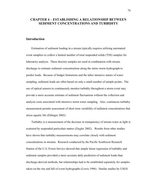
76CHAPTER 4 – ESTABLISHING A RELATIONSHIP BETWEENSEDIMENT CONCENTRATIONS AND TURBIDITYIntroductionEstimation of sediment loading in a stream typically requires utilizing automatedevent samplers to collect a limited number of total suspended solids (TSS) samples forlaboratory analysis. These discrete samples are used in combination with streamdischarge to estimate sediment concentrations along the entire storm hydrograph topredict loads. Because of budget limitations and the labor intensive nature of watersampling, sediment loads are often based on only a small number of sample points. Theuse of optical sensors to continuously monitor turbidity throughout a storm event mayprovide a more accurate estimate of sediment fluctuations without the collection andanalysis costs associated with intensive storm water sampling. Also, continuous turbiditymeasurement permits assessment of short term variability of sediment concentrations thatstress aquatic life (Ehlinger 2002).Turbidity is a measurement of the decrease in transparency of stream water as light isscattered by suspended particulate matter (Ziegler 2002). Results from other studieshave shown that turbidity measurements may correlate closely with sedimentconcentrations in streams. Research conducted by the Pacific Southwest ResearchStation of the U.S. Forest Service showed that simple linear regression of turbidity andsediment samples provided a more accurate daily prediction of sediment loads thandischarge-derived methods, but relationships had to be established separately for samplestaken on the rise and fall of event hydrographs (Lewis 1996). Similar studies by USGS

77on the Kansas River produced sediment-turbidity relationships that explained 99% of themodel variance (Christensen et al. 2002). Statistical analysis of relationships establishedfor the Little Arkansas River showed that collection of 35 to 55 sediment samples wassufficient to formulate a model, and that outliers exceeding two standard deviations fromthe mean required further investigation for potential equipment malfunction (Christensenet al. 2000).Benefits and Limitations of Using Turbidity to Predict Sediment LoadsUsing turbidity to predict sediment loading in streams can provide many benefits forwater research. First, turbidity accurately depicts sediment fluctuations during stormevents, providing the ability to catch concentrations due to short-term events such as bankslumping (Christensen et al. 2000). Turbidity can also be used to estimate loads forcontaminants typically bound to sediment particles, such as nutrients and bacteria(Ankcorn 2003). Battery-operated, internally-logging probes allow monitoring of remotelocations which are neglected by intensive sampling methods (Lewis 1996). The realtimenature of continuous turbidity data also permits quicker calculation of sedimentloads, and may even allow online posting of real-time sediment loads to accompanyavailable discharge data (Ankcorn 2003).However, relying entirely on turbidity predictions of sediment loads may havesubstantial limitations, including issues with equipment and physical streamcharacteristics. Optical turbidity probes can use a variety of different wavelengths,recording units, and sensor types. As stated by Ankcorn (2003), “turbidity is not an

78absolute value, but a relative value representing a qualitative measurement that can yielddifferent readings based on the method used.” Therefore, similar equipment must bedeployed at sampling locations to reliably draw comparisons between sites. Probes mustalso be calibrated frequently to prevent equipment drift, and equipment fouling can resultin the loss of data for particular storm events (Lewis 1996). Turbidity readings may varybetween streams due to water color and suspended particle size and composition(Packman et al. 1999). Organic particles have been shown to absorb light, and thereforeprovide different turbidity values than streams carrying primarily mineral soils (Lewis1996). In conclusion, although general sediment-turbidity relationships have beenreported, load predictions are best estimated by establishing relationships on a sitespecific basis.Research ObjectivesDeveloping a relationship between sediment and turbidity in Baird Creek mayprovide rapid, cost effective information on the effects of land use change in thewatershed on sediment delivery. The objectives of the study presented here were to:1) Determine relationships between sediment and turbidity in Baird Creek.2) Investigate the effects of streamflow on sediment-turbidity relationships.3) Compare sediment-turbidity relationships between upstream and downstreamsites.4) Compare turbidity-derived loads to those based on discrete sediment samples.

79MethodologyAs described in Chapter 3, established USGS methods were used for gagingstreamflow and for collecting, processing, and analyzing water samples at the USGSstation, North Branch, and South Branch sites from April to December 2004. Sampleswere collected under both event and low-flow conditions. Turbidity data were collectedon 10-minute intervals at each site using YSI-6200 multi-parameter sondes, and werereported in nephelometric turbidity units (NTU). Sondes were positioned within thestream channel at locations that were representative of the entire stream cross sectionduring both low and high flow conditions. Automated wipers on the optical turbiditysensors reduced equipment fouling.Sonde data were processed to exclude anomalous observations due to sedimentdeposition and equipment-associated false spikes in turbidity. Where spikes occurred,observations greater than three standard deviations from the running median werereplaced with the 50-minute median value. Individual sediment sample times were thenmatched to the closest corrected turbidity measurement taken by the sonde. Sampleswere coded as being collected during event or low-flow conditions. Samples takenduring a flow event were also coded for position on the rising or falling limb of thestream hydrograph based on an analysis of depth measurements. Linear regressionanalysis was then performed using Microsoft Excel 2003 and SAS 9.1 to generate thepredictive relationships between sediment and turbidity (SAS Institute Inc. 2003).Outliers were removed from the data set if the standardized residual exceeded threestandard deviations from the regression. Once final models were generated for the sites,comparisons were made between sites, between event and low-flow samples, and

80between samples taken on the rising versus the falling hydrograph positions by assigningdifferent numerical multipliers to categorical variables using the dummy variable optionfor the PROC REG procedure in SAS (Cody and Smith 1997). There were not sufficientdata to test for the significance of seasonality due to the lack of late summer and fallevent samples.Results and DiscussionEstablishing Sediment-Turbidity Relationships for the Sampling LocationsThe sonde data set for the USGS Station was inclusive from April to October 2004.Figure 4.1 shows continuous discharge, post-corrected turbidity, and TSS concentrationsfor samples taken at the USGS Station site from May 14 to June 25, 2004. This figureDischarge (cfs)45040035030025020015010050DischargeTurbidityTSS Concentration1,8001,6001,4001,2001,000800600400200TSS (mg/L), Turbidity (NTU)05/14/045/21/045/28/046/4/04DateFigure 4.1. Discharge, sediment sample concentrations, and turbidity data for the USGSStation site, 14 May – 25 June, 2004.6/11/046/18/046/25/040

81illustrates the variability of continuous turbidity observations during storm events, anddemonstrates the close correlation between turbidity and sediment concentrations.However, the graph also shows the potential for loss of data due to equipment fouling orburial, as seen in the extreme fluctuations in turbidity readings on May 29 and 30.Linear regression was used to establish the sediment-turbidity relationship at theUSGS station. Two outlying data points with residuals that exceeded three standarddeviations from the predicted line were removed from the regression. The intercept ofthe final model did not significantly differ from zero (p = 0.56); thus, the line was forcedthrough the origin. The final relationship between sediment and turbidity at the USGSStation was highly significant at the 95% confidence level (n = 53; R 2 = 0.97;p < 0.0001), and accounted for 97% of the variance (Figure 4.2):TSS mg/L = 2.0628(Turbidity NTU) Equation 4.1Due to a computer software error in the sonde equipment, no turbidity data werecollected by the North and South Branch sondes until June 8, 2004. Events occurring180016001400n = 53y = 2.06xR 2 = 0.97TSS (mg/L)1200100080060040020000 100 200 300 400 500 600 700 800 900Turbidity (NTU)Figure 4.2. Relationship between sediment concentrations and turbidity at the USGSStation site, April – October 2004 (n = 53).

82after this date were intensively sampled to generate a sufficient quantity of samples forstatistical analysis. Figure 4.3 displays continuous discharge, turbidity, TSS, and SSCconcentrations for event samples taken at the North Branch site from June 8 to June 20,2004. Data from the South Branch for this time period were compromised by sondeburial and turbidity probe malfunction. Therefore, we were unable to establish arelationship between sediment and turbidity for the South Branch site.As shown in Figure 4.3, both TSS (n = 22) and SSC (n = 19) concentrations closelyparallel turbidity measurements at the North Branch site. Because including a greaternumber of sample points improves a statistical model, a comparison was made betweenthe slopes of regression models generated separately from the two sample analysistechniques to determine if all points could be included in a single regression relatingsediment and turbidity on the North Branch. Using the dummy variable option in SAS, itwas found that the neither the regression slope (p = 0.61) nor intercept (p = 0.17) for TSSDischarge (cfs)18016014012010080604020DischargeTSSSSCTurbidity1600140012001000800600400200Sediment (mg/L), Turbidity (NTU)006/8/20046/9/20046/10/20046/11/20046/12/20046/13/20046/14/2004DateFigure 4.3. Discharge, sediment sample concentrations, and turbidity data for the NorthBranch site, 8 – 20 June, 2004.6/15/20046/16/20046/17/20046/18/20046/19/20046/20/2004

83versus turbidity differed significantly at the 95% confidence level from the equationgenerated for SSC versus turbidity. Therefore, concentrations from both sample analysismethods were combined to generate a single relationship between sediment and turbidityfor the North Branch site.Linear regression was used to establish the final sediment-turbidity relationship atthe North Branch site using all TSS and SSC sample concentrations. Two outlying datapoints with residuals that exceeded three standard deviations from the predicted line wereremoved from the regression. The intercept of the final model did not significantly differfrom zero (p = 0.40); thus, the line was forced through the origin. The final relationshipbetween sediment and turbidity at the North Branch site was highly significant at the 95%confidence level (n = 39; R 2 = 0.98; p < 0.0001), and accounted for 98% of the variance(Figure 4.4):TSS mg/L = 1.0119(Turbidity NTU) Equation 4.2180016001400n = 39y = 1.01xR 2 = 0.98Sediment (mg/L)1200100080060040020000 100 200 300 400 500 600 700 800 900Turbidity (NTU)Figure 4.4. Relationship between sediment concentrations and turbidity at the NorthBranch site, June – October 2004 (n = 39).

84Determining the Effect of Streamflow on Sediment-Turbidity RelationshipsOnce final relationships were determined between sediment concentrations andturbidity for the USGS Station and North Branch sites, comparisons were made betweenevent and low-flow samples and between samples taken on the rising versus falling limbof event hydrographs. Statistical analysis of event versus low-flow samples found nosignificant difference at either the USGS Station (p = 0.45) or North Branch (p = 0.21)sites at the 95% confidence level. Similarly, the analysis of rising versus fallinghydrograph showed no significant difference at the USGS Station (p = 0.14) or NorthBranch (p = 0.74) sites. Therefore, streamflow had no significant impact on therelationship between sediment concentrations and turbidity at either sampling location.Comparing TSS-Turbidity Relationships between SitesThe USGS Station site showed an approximately 2:1 relationship between sedimentconcentrations (mg/L) and observed turbidity (NTU), while the relationship established atthe North Branch site was approximately 1:1. Statistical analysis showed that therelationships significantly differed from each other at the 95% confidence level(p < 0.0001). When compared to sediment-turbidity relationships established for twoother streams within the Lower Fox River watershed, it was interesting to note that therelationships at the two Baird Creek sites showed the greatest difference despite beinglocated within one mile of each other on the same channel (Randerson et al. 2005).

85Comparing Sediment Loads for Turbidity-Derived Predictions to TraditionalMethodsUSGS predicts stream constituent loads by relating stream discharge to individualsample concentrations using Graphical Constituent Loading Analysis System (GCLAS)software (Blanchard and Miller 2004). To evaluate the reliability of turbidity-derivedloads compared to those calculated with the USGS method, loads were calculated usingthe sediment-turbidity relationship at the USGS Station site for the period of June 9-20,2004, which included five storm events. Figure 4.5 shows precipitation, discharge,turbidity, TSS sample concentrations, GCLAS predicted sediment concentrations, andturbidity-predicted sediment concentrations at the site during the study period. Table 4.1displays daily loads as calculated by the turbidity method and USGS.Table 4.1. Mean daily discharge and sediment loads predicted by turbidity and USGSGCLAS software for the USGS Station Site, 9 – 20 June, 2004.DateMean DailyDischarge (cfs)Turbidity-PredictedSuspended Solids Load,metric tonsUSGS GCLASSuspended Solids Load,metric tonsPercentDifference06/09/04 84.1 173.7 102.5 + 69%06/10/04 105.0 37.8 29.9 + 26%06/11/04 154.2 59.9 147.0 - 59%06/12/04 155.7 89.4 111.6 - 20%06/13/04 138.8 61.9 51.0 + 21%06/14/04 108.2 12.2 11.4 + 7%06/15/04 73.8 3.8 4.3 - 11%06/16/04 50.7 3.0 2.4 + 28%06/17/04 99.7 123.9 57.5 + 115%06/18/04 81.0 11.6 7.7 + 50%06/19/04 67.9 4.1 3.9 + 5%06/20/04 47.1 1.7 1.9 - 11%Totals: 583.0 531.0 +10%

86Discharge (cfs)240220200180160140120100806040200ADischargePredicted TSSTurbidityTSS25002000150010005000TSS (mg/L), Turbidity (NTU)Discharge (cfs)240220200180160140120100806040200BDischargeActual TSS ConcentrationEstimated TSS ConcentrationGCLAS Estimated Concentration25002000150010005000TSS (mg/L), Turbidity (NTU)Hourly Precip. (mm)1614121086420C1009080706050403020100Cumulative Precip. (mm)Cumulative Precip. (mm)6/8/04 0:006/9/04 0:006/10/04 0:006/11/04 0:006/12/04 0:006/13/04 0:006/14/04 0:006/15/04 0:006/16/04 0:006/17/04 0:006/18/04 0:006/19/04 0:006/20/04 0:00Date - TimeFigure 4.5. Comparison of turbidity-predicted and GCLAS estimated sedimentconcentrations for the USGS Station Site, 8 – 20 June, 2004: (a) discharge,sediment samples, turbidity-predicted continuous sediment concentrations,and turbidity data, (b) discharge, sediment samples, and GCLAS estimatedcontinuous sediment concentrations, and (c) hourly and cumulativeprecipitation data.

87Daily loads differed substantially between the two methods during the period ofevents. In comparing Figures 4.5A and 4.5B, it was evident that the limited number ofwater samples collected on June 11 and 12 led to difficulties in estimating fluctuations instream sediment concentrations. The USGS load prediction for these two days was basedon interpolating sediment concentrations from the single sample point from June 12 andrelatively similar daily discharges, leading to substantial overestimation of loads on June11. Estimates based on turbidity for the June 11 event were significantly lower and maybe explained by examining discharge. The slow rise of the hydrograph over the previousday and the June 11 event may have resulted from exceeding the storage capacity of theheadwaters wetlands complex, thus resulting in relatively low sediment concentrations inthe stream. Comparisons between Figures 4A and 4B for the events of June 9 and June17 also indicated that the first-flush of these intense storm events may have carried moresediment than estimated by USGS based on the limited number of sample points.Despite daily differences in load prediction between the two methods, turbiditybasedload estimates for the entire time period were within 10% of the loads calculatedby USGS. Therefore, monitoring turbidity in conjunction with limited water samplingappears to be a reasonable surrogate for sediment-discharge predictions in loadestimation on a weekly or monthly basis.ConclusionsThe turbidity of Baird Creek is highly dynamic. Sharp increases in turbidity wereclosely associated with runoff events and changes in stream discharge. Linear regression

88analysis showed a strong relationship between sediment concentrations and turbidityreadings in Baird Creek at both stations, accounting for 97-98% of the model variance.However, no significant difference was found due to event versus low-flow samples ordue to hydrograph position. The effect of seasonality was not analyzed due to lack ofdata from late summer and fall storm events and equipment malfunction.The relationship between sediment concentrations and turbidity significantly differedbetween the upstream and downstream sampling sites. We hypothesize that thedifference between these two models is directly related to watershed land use and theassociated hydrologic response between the primarily agricultural North Branch site andthe urban storm water additions above the USGS station. As discussed in Chapter 3,significant sediment load from urban tributaries and bank erosion enters Baird Creekbelow the North Branch monitoring station. The higher proportion of large-sizedparticles (e.g. sand) from these sources may be influencing the refraction of light throughthe water column and thus the turbidity sensor response, as compared to that of the siltand clay-sized suspended sediment carried from the agricultural watershed.Continuous turbidity monitoring appears to be a reasonable surrogate for sedimentconcentration prediction for Baird Creek, and may provide cost effective, rapidlyavailable information on watershed sediment delivery due to changes in land use. Futureresearch on suspended particle properties and size distributions would assist inunderstanding site-to-site differences in the sediment-turbidity relationships.Relationships could also be strengthened by selecting samples for sediment analysisbased solely on the real-time turbidity data, thus completing the curve with well-spacedsamples throughout the full range of observed turbidity (Lewis 1996). Additional

89opportunities for further study include assessing seasonal variability and refining sondedeployments to lessen false spikes and/or equipment fouling.