SEISMIC ANALYSIS AND SHAKE TABLE MODELING: USING A ...

SEISMIC ANALYSIS AND SHAKE TABLE MODELING:USING A SHAKE TABLE FOR BUILDING ANALYSIS.bySandra BrownA Thesis Presented to theFACULTY OF THE SCHOOL OF ARCHITECTUREUNIVERSITY OF SOUTHERN CALIFORNIAIn Partial Fulfillment of theRequirements of the DegreeMASTERS OF BUILDING SCIENCEMay 2007Copyright 2007Sandra Brown

DedicationThis thesis is dedicated to Erik Novales, for all of hissupport and encouragement, and to my parents, Stacyand Joseph Brown.ii

AcknowledgementsThis thesis would not have been possible without the guidance and dedication of mythesis committee members. Professor Goetz Schierle provided the inspiration andthe commitment to continue on, and Joseph Pingree provided expertise andknowledge in subjects foreign to me. Professor Doug Noble kept me on track, andProfessor Marc Schiler kept me honest. From all of these people, I learned a greatdeal.iii

AbstractThis Thesis is about the process of rehabilitating a shake table for use in seismicanalysis of small-scale models in the School of Architecture. Labview 8.0 StudentEdition was used to write the controlling program for the shake table.In order to test seismic response of a prototype building, a 7-story reinforcedconcrete building was modeled in piano wire and plywood and tested on the shaketable. The shake table recorded data from an accelerometer mounted on the model.The model was built to have the same resonant frequency as the prototype building.The model clearly shows modal forms and shows exaggerated deflection, as well astorsion caused by modeling inconsistencies. Reactions in the model correlate to theprototype. A model on a shake table is useful to the School of Architecture as ateaching tool to visually highlight the effect strong ground motion can have on abuilding.Keywords: Shake Table, Labview 8.0, Seismic Analysis, Teaching Tool, SeismicModeling.iv

Table of ContentsDedication.................................................................................................iiAcknowledgements ................................................................................ iiiAbstract....................................................................................................ivTable of Figures and Tables ................................................................. viiiChapter One: Introduction.......................................................................1Thesis Outline ......................................................................................................... 11.2 Seismology........................................................................................................ 21.3 Lateral Forces................................................................................................... 41.4 Damages from Seismic Forces.......................................................................... 51.5 Model Testing ................................................................................................... 61.6 Shake Tables ..................................................................................................... 71.7 Understanding versus Memorization ................................................................ 81.8 How to use the results of this research.............................................................. 91.9 Definitions of terms and formula .................................................................... 10Chapter 2: Seismic Forces and Shake Table Analysis ..........................142.1 Faults............................................................................................................... 142.2 Seismic Forces ................................................................................................ 172.3 Building reaction to Seismic Forces ............................................................... 202.4 Model Analysis ............................................................................................... 232.5 Shake Tables ................................................................................................... 232.6 G G Schierle Shake Table............................................................................... 242.7 Previous Work at USC.................................................................................... 25Chapter 3: Methodology........................................................................283.1 The G. G. Schierle Shake Table...................................................................... 283.2 Amplifier......................................................................................................... 303.3 Digital/Analog Converter................................................................................ 343.4 Labview 8.0 Student Version.......................................................................... 343.5 Shaker.............................................................................................................. 35v

3.6 Earthquake Data.............................................................................................. 363.7 Building the Model ......................................................................................... 363.8 Contingency Plans........................................................................................... 36Chapter 4: Fixing the Shake Table ........................................................384.1 Original Condition .......................................................................................... 384.2 Procedure for Fixing the Shake Table............................................................. 394.3 Software .......................................................................................................... 504.4 Problems.......................................................................................................... 524.5 Troubleshooting .............................................................................................. 52Chapter 5: Building a Test Model .........................................................545.1 Types of models already in use....................................................................... 545.2 Selecting a Model Type .................................................................................. 555.3 Modeling a Real Building ............................................................................... 565.4 Symbols........................................................................................................... 595.5 Calculations..................................................................................................... 605.6 Building the Model ......................................................................................... 635.7 Fixing the Model to the Shake Table .............................................................. 655.8 Testing............................................................................................................. 66Chapter 6: Running a shake table test ...................................................686.1 Installing the Model ........................................................................................ 686.2 Selecting an earthquake data file..................................................................... 716.3 Verifying Input and Output results ................................................................. 736.4 Running the test .............................................................................................. 746.5 Possible Problems ........................................................................................... 77Chapter 7: Results and Analysis............................................................807.1 Introduction of Testing.................................................................................... 807.2 Verification Tests............................................................................................ 827.3 Model Testing and Results.............................................................................. 87vi

Chapter 8: Conclusions........................................................................1008.1 Correlations to prototype building data......................................................... 1018.2 Concluding Remarks..................................................................................... 102Chapter 9: Future Work.......................................................................1039.1 3-Degree of Motion Shake Table.................................................................. 1039.2 Different Modeling Techniques .................................................................... 1039.3 Soils Testing.................................................................................................. 1049.4 Calibration..................................................................................................... 1059.5 Better Measurement Devices ........................................................................ 1059.6 More Earthquake Files .................................................................................. 1069.7 Earthquake Remediation Strategies .............................................................. 1069.8 Strategies for use as a teaching tool ........................................................ 107Bibliography .........................................................................................109Appendix A : Instructions for Using Labview ....................................111Appendix B: Index of Videos Submitted .............................................114vii

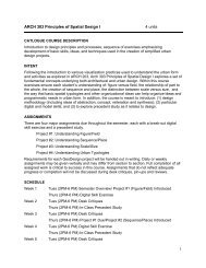
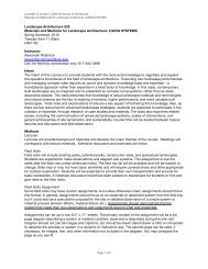
Table of Figures and TablesFigure 1.1: Fatalities of Major Earthquakes 1970-1999 (Schierle 2005 pg 29) ........ 3Figure 1.2: 10 Freeway at Venice Blvd. after Northridge. ......................................... 5Figure 1.3: G G Schierle Shake Table with testing model......................................... 7Figure 1.4: G. G. Schierle Shake Table ................................................................... 11Figure 1.5 National Instruments USB-6008, Digital Analog Converter,.................. 12Figure 1.6 Labview Interface Front Screen............................................................... 13Figure 2.1: Major Tectonic Plate Boundaries .......................................................... 14Figure 2.2: Types of Faulting in the Earth's Crust ................................................... 15Figure 2.3: Earthquake Faults in Southern California ............................................. 16Figure 2.4: Types of Earthquake Waves.................................................................. 19Figure 2.5: An example of earthquake damage in the 1994 Northridge Earthquake............................................................................................................................ 22Figure 3.1 The G. G. Schierle Shake Table. ............................................................ 29Figure 3.2: Picture of fuse used to replace broken fuses........................................... 31Figure 3.3: A Male BNC Connector used in connecting the digital analog converterto the amplifier. ................................................................................................. 32Figure 3.4: The back of the amplifier ....................................................................... 33Figure 3.5: The Shaker Component of the Shake Table. ......................................... 35Figure 4.1: Block Diagram showing how the shake table components connect toeach other. ......................................................................................................... 40Figure 4.2: Shaker Component 3-Pin Connector Diagram ...................................... 42Figure 4.3: Circuit designed by Joseph Pingree for DAC........................................ 43Figure 4.4: Diagram of the Pin Connections in the TL082 Op Amp that was used tomake the DC to DC converter added to the DAC............................................. 43Figure 4.5: Image of the DAC inside a custom metal box....................................... 44Figure 4.6: The author soldering the circuit to convert a positive voltage to a +/-voltage............................................................................................................... 44Figure 4.7: Functional Block Diagram from Analog, Inc........................................ 45Figure 4.8: The Pin Diagram for the Accelerometer, from Analog Devices, Inc.... 46Figure 4.9: Circuit design for the amplifying circuit of the accelerometer.............. 47Figure 4.10: The amplifying circuit tested on a breadboard. ................................... 48Figure 4.11: Oscilloscope, and Joseph Pingree testing the circuit of theaccelerometer and amplifier.............................................................................. 49Figure 4.12: The amplifier and the accelerometer mounted to the shake table andconnected to the DAC with wires and Molex Connectors................................ 50Figure 4.13: Labview Front Page............................................................................. 51Figure 5.1: Locations of the CR-1 recording system in the Van Nuys Building.Image credited to Prof. Trifunac at USC. ......................................................... 58Figure 5.2: Compressive Strength of the Columns in the Prototype Building. ....... 61Figure 5.3: Critical loading for the columns in the prototype building. .................. 62Figure 5.4: Slenderness ratio for columns in the prototype building........................ 62Figure 5.5: Model dimensions, section. ................................................................... 64viii

Figure 5.6: Shake Table Plan for Mounting Models (Units in Inches).................... 65Figure 5.7: Diagram of Bracing in Prototype Building. (Trifunac 2001 pg. 15) .... 67Figure 6.1: Screen shot of Simulated File Controls .................................................. 70Figure 6.2: Lead fishing weights used for model testing......................................... 71Figure 6.3: Data Extracting Program ....................................................................... 73Figure 6.4: Input and Output graphs ......................................................................... 74Figure 6.5: Labview File Input ................................................................................ 74Figure 6.6: Timing Parameters................................................................................. 75Figure 6.7: Illustration of "Run" Button .................................................................. 76Figure 6.8: The Stop Button..................................................................................... 76Table 7.1: Table of Tests run on the Shake Table.................................................... 82Table 7.2: Accelerometer test 6-8. ........................................................................... 83Table 7.3: Test 11, paper displacement tests............................................................ 83Table 7.4: Test of Noise Filters in the Input of the Accelerometer data.................. 84Table 7.5: Input/Output verification test at 1 Hz ..................................................... 85Table 7.6: Tests 18, 19, and 20, Roof ...................................................................... 87Table 7.7: Prototype Building Roof Reaction to Northridge Earthquake 1994....... 88Table 7.8: Tests 18, 19, and 20 5th Floor................................................................. 90Table 7.9: Prototype Building 5th Floor Reaction to Northridge Earthquake 1994.91Table 7.10: Model Test 3rd Floor Reactions ........................................................... 92Table 7.11: Model Test 2nd Floor............................................................................ 93Table 7.12: Model Test of Bracing- roof reaction ................................................... 95Table 7.13: Bracing on the Model- 5th Floor .......................................................... 96Table 7.14: Model Bracing Test- 3rd Floor ............................................................. 97Table 7.15: Bracing Test 2nd Floor ......................................................................... 98Figure 9.4: Types of eccentric braced frames ........................................................ 107Figure A.1: Labview Front Page............................................................................ 112Figure A.2: Labview Block Diagram..................................................................... 113ix

Chapter One: IntroductionThe University of Southern California’s School of Architecture G. G Schierle shaketable can be used in a meaningful way to study a building’s seismic response usingexisting seismic data. The G. G Schierle Shake Table is an important teaching toolthat is useful to show aspiring architects and engineers how a structure will respondin a seismic event. With first an understanding of how the shake table was damaged,as well as an update in the controller interface for the shake table, the Schierle ShakeTable was fixed and is once again operational. Since the shake table is nowoperational and updated, models are used to test the shake table and calibrate thecontrolling program and devices.Thesis OutlineIn Chapter 2, the causes of earthquakes and the history of seismic modeling on ashake table will be discussed, as well as previous research using the Schierle ShakeTable.In Chapter 3, the methodology of modeling a specific building on the shake tablewill be examined, as well as an explanation of how the shake table components worktogether to simulate a seismic event.Chapter 4 comprised documentation of how the shake table was actually fixed, andhow all the components work together.1

In Chapter 5, the modeling technique used as well as the guidelines for selectingmodeling materials were explained.In Chapter 6, the process of running the experiment was described. Possibleproblems were listed and potential solutions were listed.In Chapter 7, the findings of the actual test of the seismic model were documented.The model were tested using the 1994 Northridge Earthquake data and tested thecase study building’s deflection prior to the seismic bracing and following theaddition of the seismic bracing.Chapter 8 evaluated the relevance of the data from the test to determine if futuretests in this manner will yield reliable results.Chapter 9 summarized and concluded the findings.Chapter 10 comprised suggestions for future work.1.2 SeismologySeismology is a relatively recent field of study. Seismology is the study ofearthquakes, which are caused mostly by plate tectonics, the huge pieces of theearth’s crust as they move relative to each other, which causes strain in the2

intersecting fault lines. One of the major plate boundaries occurs in California at theboundaries of the Pacific Plate and the Continental Plate; known as the San AndreasFault. This is a strike slip fault, meaning it moves laterally along the fault. Thestudy of earthquakes is important because earthquakes cause billions of dollars indamage every year around the world, and thousands of deaths and tens of thousandsof injuries. In the United States, around 1,200 deaths have been recorded since1900. Many more fatalities occurred in earthquakes elsewhere, see fig. 1.1. Mostdeaths in earthquakes are caused when a structure collapses (Congress 1995 pg 6).Figure 1.1: Fatalities of Major Earthquakes 1970-1999 (Schierle 2005 pg 29)3

1.3 Lateral ForcesThe strong lateral movement caused by a seismic event can cause structural damageto a building. Buildings are designed for gravity, and thus are usually sufficientlydesigned for vertical movement. Lateral movements, however, can cause largeshear forces to the walls, introduce bending to columns, and torsion if the center ofmass and center of resistance are offset. Most structural failure is due to buildingsnot having enough bracing or shear resistance or moment resistance. Structures ofbrittle material are more vulnerable than structures of ductile material.More recently, research from the 1994 Northridge event has led to a re-evaluation ofthe assumption that lateral forces are the governing forces in terms of buildingdamage in seismic events. Strong vertical forces over the epicenter of the eventcaused damage to freeway pillars on the Santa Monica Freeway, leading to crushingof the pillars. Strong lateral forces in addition to strong vertical forces that introducepounding to columns and can lead to containment issues in concrete beams andcolumns. See Figure 1.2 for a picture of the 10 Freeway at Venice Boulevard, justafter the Northridge event.4

Figure 1.2: 10 Freeway at Venice Blvd. after Northridge.1.4 Damages from Seismic ForcesEarthquake forces act similarly to sound waves, in the way they propagate throughthe soil. They can be produced at different frequencies and at different amplitudes.Large earthquakes tend to produce larger amplitude, lower frequency seismic waves,whereas small earthquakes tend to have smaller amplitudes but higher frequencywaves. This is, however, only a generalization, as each earthquake has a variety ofcomplex waveforms of various amplitudes and frequencies. The damage done tostructures depends mostly on the interaction between soil and structure and howthese waves hit the structure. Seismic waves can move vertically, horizontally, or acombination of both, and can come from any direction. Higher frequency5

earthquakes tend to damage shorter, stiffer structures, and lower frequencyearthquakes tend to damage taller, more ductile structures. Buildings with the sameperiod of a seismic event tend to resonate and be more damaged. Buildings have aresonant period of about 0.1 second per story, so a 10-story building would have aresonant period of 1 second.1.5 Model TestingGiven the failures due to eccentricity, insufficient strength, etc., it is important thatarchitects understand the potential hazards in their design and understand where thebuilding needs to be braced. Testing of models of actual buildings and buildingprototypes is one method that is useful in understanding the forces at work. Modelsbuilt of plywood and steel wire allow students to see the seismic behavior of astructure, and to understand how the period of an earthquake if it is resonant with abuilding period, will cause the most damage or even collapse. Models may be testedon a shake table or in a computer program. However, shake tables are moreeffective as a teaching tool to simulate seismic behavior because they most closelysimulate human error in the construction process and allow for easy understandingof the building reaction to the seismic forces.6

1.6 Shake TablesThe shake table is a device that simulates a seismic event. It can also be used tocreate fictional “worst case” scenarios or resonant frequencies. In computercontrolled shake tables a computer program generates a signal, and a digital signal issent to a digital/analog converter, which sends a voltage to the amplifier. Theamplifier amplifies the voltage and sends it to the shaker platform to which themodel is attached. The Schierle Shake Table is a one-degree of motion shake table,meaning that it will move only in one lateral direction.Figure 1.3: G G Schierle Shake Table with testing model.7

A model on a shake table with the same stiffness or resonant frequency as theprototype building, will act in a way similar to that of the actual building.Mathematical equations and formula alone are not effective to convey seismicbehavior to students. In a hands-on pedagogical method, such as a model on a shaketable, students see the effects of seismic forces on a building and are better preparedto apply the formula learned to an actual situation. Students then have betterunderstanding of structures and a greater respect for seismic forces.1.7 Understanding versus MemorizationIn an abstract teaching system, students are given formulae and facts to memorize,sometimes with a lack of fundamental understanding of the physical laws behind theformula. In a professional school such as architecture, students are required to takethe knowledge from school and apply that to the creation of a building. As anyarchitect knows, no two buildings are exactly alike, and each site and building posenew challenges. Rote memorization does little to prepare a student for applicationof knowledge to a unique and specific challenge. Only a fundamental understandingof the knowledge allows one to apply the correct formula or equation to the rightproblem. Eric Mazur, of Harvard University’s Department of Physics, wrote a paperabout physics students’ lack of understanding of memorized problems. Hediscovered in his physics classes that peer instruction and physical demonstrationsgreatly improved student understanding of physic concepts (Mazur 1995 pg. 5).Mazur compared the students’ final examination scores from a class he taught8

conventionally, and the same final examination given to students taught via peerinstruction and physical demonstrations. The students taught with the hands-onprocess scored much higher than the conventionally taught students (Mazur 1995 pg.7). Students in classes taught with peer instruction and in class demonstrationsscored 30 to 70% higher on average than students taught in a traditional class(Mazur 1999 pg. 3).1.8 How to use the results of this researchStudents in the structural classes in the School of Architecture at the University ofSouthern California will be able to build models of their architectural projects fortesting in a seismic event. A student would then be able to see that form (modelsare not of the real material) has a large effect on how a building will react to seismicforces, and then be able to make informed decisions on how best to proceed withtheir design.Students will also be able to build simple models to test the effects of earthquakebracing on a general building, or test seismic dampeners. Students will gain anintuitive sense of how a building will react, and can use this teaching tool as a wayto create new and innovative ways of dealing with an unpredictable and damagingnatural disaster.9

1.9 Definitions of terms and formulaShake Table: The shake table is the G. G Schierle Shake Table located in theMasters of Building Science Laboratory consists of a Digital/Analog converter, APSDynamics Electro-Seis shaker model 113 and an APS Dynamics amplifier model114 and a platform suspended from a steel frame. It was originally built in 1981 andwas intended to be used as a teaching tool in the School of Architecture. It has asteel frame and a wooden platform for the amplifier and the controlling computer.The shaker is bolted to the base of the frame, and connected to an aluminumplatform with a long bolt. The platform is suspended from the top of the frame withcables and cross-braced to reduce the introduction of torsion into the model. Theplatform has holes drilled 3” on center regularly spaced in a grid, for ease ofsecuring models for tests. The whole frame is 5’ tall, and 3’ wide.10

Figure 1.4: G. G. Schierle Shake Table11

Digital/Analog Converter:The digital/analog converter is a National Instruments USB-6008 DAC that takes adigital signal and converts it to a voltage for use with the amplifier.Figure 1.5 National Instruments USB-6008, Digital Analog Converter,(http://sine.ni.com/nips/cds/view/p/lang/en/nid/14604)12

Labview 8.0, Student Version: Labview is a graphic programming language sold byNational Instruments. It uses the C programming language in a graphic way tocontrol testing instrumentation.Figure 1.6 Labview Interface Front ScreenThe next chapter explores the background of seismic events and modeling.13

Chapter 2: Seismic Forces and Shake Table AnalysisThis chapter will cover the following four things: what earthquake and seismicevents are and how they work, how buildings respond to those forces, what the G. GSchierle Shake Table is, and the previous research at USC using the shake table.2.1 FaultsAn earthquake occurs when built up energy is released in a sudden slippage of afault. Faults, or cracks in the earth’s surface, occur primarily at the edges of tectonicplates, large pieces of the earth’s crust. (Fig. 2.1). There are three types of faults:Normal, Reverse, and Strike Slip Faults (Fig. 2.2).Figure 2.1: Major Tectonic Plate Boundarieshttp://www.cev.washington.edu/lc/CEVIMAGES/global-techtonic-plates.jpg14

Normal faults are faults where the hanging wall, the side of the fault that hangs overthe fault, moves downward in relationship to the footwall. An example of a normalfault is the Mid-Atlantic Ridge, a spreading plate boundary.Figure 2.2: Types of Faulting in the Earth's Crusthttp://earthquake.usgs.gov/images/faq/3faults.gifReverse Thrust Faults are faults where the footwall moves upward in relationship tothe hanging wall. An example of a reverse thrust fault is the Sierra Nevada Faultzone, which has caused the Sierra Nevada mountain range in California.15

Strike Slip faults are the faults most relevant to Southern California. A Strike Slipfault is a fault in which one side of a fault moves horizontally in relationship to theother side of the fault typically parallel to the fault. The San Andreas Fault Systemthat forms part of the boundary between the North American Plate and the PacificPlate is a Strike Slip fault. Strike Slip Faults are either Right Lateral Faults,meaning that one side of the fault moves from left to right in relationship to a vieweron the opposite side of the fault, or Left Lateral Faults, in which the motion of thefault moves from right to left in relationship to a viewer on the opposite side of thefault. See Figure 2.3 for more information on the faults specific to SouthernCalifornia.Figure 2.3: Earthquake Faults in Southern Californiahttp://www.earthquakecountry.info/roots/inline/11839sm.jpg16

The San Andreas Fault, which is responsible for some of the largest earthquakes inCalifornia’s history, is a left lateral strike slip fault. A rupture on the southern partof the San Andreas Fault could unleash an earthquake upwards of Magnitude 8.0.There are no measurements of any earthquakes occurring on the lower part of theSan Andreas Fault. The last known earthquake was the 1857 Fort Tejon Earthquake,with a recorded Modified Mercalli intensity from X to XI, with a peak groundacceleration of more than 0.60g, where g = gravity acceleration.. Almost all unreinforcedmasonry buildings were destroyed and the ground badly cracked. Therewas a 9-meter displacement, and the fault ruptured for 300 miles, from Parkfield toWrightwood, California. Two buildings were destroyed and three were heavilydamaged and considered uninhabitable at the army outpost of Fort Tejon.2.2 Seismic ForcesWhen a fault ruptures, it releases a large amount of stored energy. This energyradiates out from the epicenter, the point on the earth’s surface where the rupturestarts. There are four types of waves. Two of the three are called body waves,which propagate within a body of rock and radiate out from the epicenter of theearthquake. The two body waves are P-waves, and S-waves. The third and fourthtypes of waves are surface waves, the Love wave and the Rayleigh wave.P-waves, or primary waves, are the fastest waves, and are compression waves,meaning they have a push and pull type of motion. P-waves act similarly to sound17

waves, and move through both solid rock and liquid material. S-waves, orsecondary waves, are shear waves that shear the rock sideways at right angles to itsdirection of travel. These waves are slower than P-waves, and cannot travel throughliquid. While P-waves act like sound waves, the S-wave acts more like a sine wave(Fig. 2.4).18

Figure 2.4: Types of Earthquake Waveshttp://www.darylscience.com/graphics/seiswave.gif19

When an earthquake occurs, the high-speed P-waves are felt first, in an effect thatrattles windows and can sometimes sound like a sonic boom. The S-waves arrivewith a vertical displacement and a lateral displacement, and are the waves mostlikely to damage a building. (Bolt 2004 pg. 20) The time lag between wave arrivalsdefines the distance of an earthquake. The distance from three seismic stationsdefines the epicenter location. Surface waves travel near the earth surface.There are two types of surface wave, the Love wave and the Rayleigh wave. Lovewaves have a side-to-side movement along the horizontal plane of the earth’ssurface. It has no vertical displacement, and this horizontal shaking is particularlydamaging to a building’s foundations. The Rayleigh wave acts more like an oceanwave, with an elliptical motion both vertically and horizontally in a vertical plane inthe direction of wave propagation. These surface waves are usually much slowerthan the body waves, and in an earthquake, the first moments of shaking are bodywaves, followed then by Love waves, which are faster than Rayleigh waves.2.3 Building reaction to Seismic ForcesTypically, an earthquake can cause four types of damage to a building. A buildingcan collapse, which can result in the total loss of the building and possibly the livesof the occupants. A building can suffer structural damage, which leaves the buildingstanding, but unsafe, and either results in the eventual demolition of the building orexpensive remediation costs to repair the structural damage. A building may also20

suffer non-structural damage to walls, water pipes, windows, and so forth. Thesecosts can be expensive to repair, but are preferable to losing lives. Non-structuraldamage usually amounts to over 70 percent of total damage (Schierle, 2001, p.1-1).Lastly, a building might suffer damage to the contents inside, which result fromobjects not being properly anchored to walls or otherwise properly secured.(Congress 1995 pg. 8)Engineers and architects hope that a building in a seismically active area wouldsuffer minimal damage, but of the four types, a designer would prefer cosmeticdamage to structural damage or collapse, in an effort to preserve life safety. Ofcourse, architects would prefer no damage, but due to the nature of seismisivity,earthquakes are unpredictable, vary in terms of magnitude, strength, period, andpeak ground acceleration. No two earthquakes are alike, and the effects ofearthquake strength can still surprise engineers and seismologists.21

Figure 2.5: An example of earthquake damage in the 1994 Northridge Earthquake.This is a parking structure in Northridge that collapsed, showing the ductility in the concrete.http://www.calstatela.edu/dept/geology/earthquakes/CSUNParking(2).jpgPrimarily, architects and engineers are concerned with the lateral forces thatearthquakes generate. The rationale is that structural engineers already design forvertical gravity dead loads and live loads. Because designers include a safety factorto compensate for unexpected loads in the vertical direction, it is assumed thatvertical forces are not necessarily the problem in an earthquake. Therefore, lateralforces tend to govern earthquake resistant design in building codes and in practice.As a note of caution to designers, directly over the epicenter in the Northridge event,strong vertical acceleration was recorded, and the resulting combination of strongvertical and lateral forces caused loss of containment in the concrete columnssupporting freeways and buildings.22

2.4 Model AnalysisModel Analysis is the use of physical or computer models to test shaking orvibration of an object. Architects and engineers use equations defined by codes todetermine the resonant period of a structure, which is useful to know because abuilding will suffer the most physical damage during a seismic event that has thesame frequency as the resonant building frequency. If models are used they musthave similitude to the actual structure that is being studied. A model is said to havesimilitude with an actual structure if it has similar geometry, dynamic properties,and period. Geometric similarity means that the model is a scaled down version ofthe actual building, in the same shape. Dynamic similarity means that the ratios ofall forces acting on the building are consistent.2.5 Shake TablesPrior to the invention of the seismograph in 1880, there was no way to accuratelytest a seismic event. With the invention of the Richter Scale in 1935, there was away to measure and compare earthquakes. In the aftermath of the 1906 earthquakein San Francisco, earthquake research in the United States of America was pushed tothe forefront of geologic studies in California. Two universities in the San Franciscoarea, Stanford University and the University of California, Berkeley made majorresearch gains documenting the effects of the earthquake and the aftermath thereof.23

2.6 G G Schierle Shake TableBecause architects are primarily concerned with the lateral forces added to abuilding in a seismic event, the University of Southern California Chase LeavittGraduate Building Science Program has a shake table to visually analyze the effectsof a seismic event to a building model. The Schierle Shake Table is a one-degree ofmotion shake table, built by Professor Schierle and students. The shake tableincludes:• Steel frame• Computer• Suspended aluminum shaker platform• APS systems Electro-seis 113 shaker component• Digital/analog converter• Amplifier component is Model 114The Schierle Shake Table accepts electronic input via a digital analog converter,which is a component in the controlling computer. The amplifier takes +/- 2 voltsfrom a digital/analog converter and modulates the voltage up to 220 volts,maximum, and 4 amperes are amplified to 6 amperes. Using Labview 8.0, Studentversion, from National Instruments, Inc. to input the data and control the outputvoltage, one can send actual earthquake waveform data to the shaker to simulatebuilding response to the seismic event.24

Using a shake table for modeling building response during a seismic event is usefulto both teachers and students trying to grasp how structures respond to strong lateralforces. Students can see the deflection in a model, and see the inflection points incolumns. If one uses fabric in the model to simulate walls, a student can see actualshear forces acting on the fabric. With shake table simulation students see avisualization of the forces to help understand the building response.2.7 Previous Work at USCProfessors G. Goetz Schierle, James Ambrose, and Dimitri Vergun, and studentshave previously used the shake table to test models under seismic forces.The theses regarding the shake table in Professor Schierle’s possession are:H Iriano (1988) Response of High-rise Structures to Lateral Seismic GroundMovements S Chong (1993) Investigation of Seismic Isolators as a mass Damper forMixed Use BuildingsChong’s Thesis was the last to use the shake table.The shake table stopped working sometime thereafter.The testing was thorough, but lacks the specific information on the shake table touse to restore it. More thorough documentation on the testing equipment wouldhave been helpful to the restoration of the shake table. However, the notes on modelbuilding were thorough and helpful.25

No other work mentioning the Shake Table at USC was available.However, shake tables have been used before in academic environments. TheNetwork for Earthquake Engineering Simulation (NEES) at Berkeley, California,first built their large scale shake table in 1972. This table is 20’ x 20’, and has a 3degree range of motion. It may be used to subject structures weighing 100,000 lbsto horizontal accelerations of 1.5g. (http://eerc.berkeley.edu/lab/earthquakesimulator-lab.html).A 3 degree shake table is more accurate than the 1 degree oflateral motion, because earthquakes cause 3-degree motions that a 1 degree shaketable cannot simulate.The University of San Diego has the largest outdoor shake table. This shake table isonly a 1 degree of lateral motion shake table, and is 25’ x 40’ in dimension. SanDiego built a 65’ tall concrete building to test that less reinforcing steel is a moreeffective strategy in concrete buildings, defined as ductile design required forconcrete structures since 1976. The researchers then tested the building using the1994 Northridge earthquake event. Their findings support their hypothesis; thatexcessive building strength can actually promote poor structural performance andnon-structural damage(http://www.jacobsschool.ucsd.edu/news/news_releases/release.sfe?id=508). ANational Geographic Special described one critical flaw in their testing in that theydid not take into account the vertical movements in an earthquake, the containment26

of the concrete in the columns was inadequate, and would have led to the structuralfailure of the columns in the actual event (National Geographic 2006).Small scale testing has occurred at California State University Northridge. Smallscale testing on a shake table is not as accurate as large scale testing because of thedifficulty of scaling down the material properties of actual building materials.However, small scale testing is good regarding seismic design concepts, such asshear cracks, building deflection, torsion, and stiffness of a building. For teaching aconceptual class, such as in an architecture school, such small-scale tests are moreuseful because they can be completed in a short amount of time with a minimum ofmodel building materials.In the next chapter, a brief introduction to how the G. G Schierle Shake Tableoperates and how models can be built to test conceptual ideas will be discussed.27

Chapter 3: MethodologyChapter 2 contained the basics of why earthquakes occur, and why building modelsto test on a shake table are useful to examine how a building will roughly respond toa seismic event.3.1 The G. G. Schierle Shake TableThe G. G. S. Shake table is composed of four major components:• Steel frame• Computer• Suspended aluminum shake platform• Digital analog converter (converts a digital waveform file to a voltage)• Amplifier (amplifies a small voltage of the digital/analog converter outputsto a larger current to control the shaker)28

Figure 3.1 The G. G. Schierle Shake Table.29

3.2 AmplifierThe amplifier takes a voltage of +/- 2 volts maximum input, and amplifies thevoltage up to +/- 220 volts, maximum output needed to activate the shake table. Theamplifier draws 300 Watts of initial Input Power, and amplifies the current from 4amps to 6 amps. The amplifier draws 1320 maximum Watts. The amplifier, inorder to work properly, needed to be thoroughly dusted and cleaned, and the fusesthat regulate the input voltage and current needed to be checked and replaced. Theamplifier uses two glass fuses, 250V 4 amp. The current fuse used is an SOC SS2(Figure 3.2). This fuse is a fusible link made of glass and ceramic to protect againstcurrent surge. The amplifier is connected to the Digital Analog Converter using aBNC connector. The BNC connector is a type of RF connector used for terminatingcoaxial cable (Figure 3.3).30

Figure 3.2: Picture of fuse used to replace broken fuses.31

Figure 3.3: A Male BNC Connector used in connecting the digital analog converter to theamplifier.http://upload.wikimedia.org/wikipedia/commons/thumb/a/a0/BNC_connector.jpg/639px-BNC_connector.jpgThe amplifier has two circuit boards inside, two capacitors, and a large heat sink andfan. Using a voltmeter and a multimeter, the digital analog converter sent a testvoltage to the amplifier using the test functions of the digital analog converter to testthe signal in the amplifier. A multimeter is an electronic measuring instrument thatcombines several functions in one unit. The most basic instruments include anammeter, voltmeter, and ohmmeter. A voltmeter measures only voltage in a circuit.32

The test function option will automatically pop up on the computer screen when oneplugs the USB cable of the digital analog converter into the USB port.Figure 3.4: The back of the amplifierNote the large cooling fan and the circuit that controls the input and output power. In themulticolored ribbon cable, the orange, yellow, and brown wires seem to handle the input voltage..Figure 3.4 shows the large cooling fan and the circuit that controls the input andoutput power. In the multicolored ribbon cable, the orange, yellow, and brown wiresseem to handle the input voltage. Follow the orange, yellow, and brown wires in the33

amplifier circuitry to assure that the voltage is properly flowing from the input andto the output cables. The color-coding seems consistent throughout the amplifier,however, not all wires were tested and these colors may not be the only wires tocarry voltage and current. There will be a maximum of 42 volts at the capacitors ifthe circuitry is working properly. The amplifier needs be grounded to the casing.With the red probe of the multimeter, switched to voltage, verify that there is 42volts at the blue capacitors. The black probe should be attached to the case, which isgrounded.3.3 Digital/Analog ConverterThe digital/analog converter used is a National Instruments USB 6008. This deviceconverts a digital signal, i.e. a waveform, into an analog signal, or a voltage. TheUSB device connects to a computer using a USB cable. The device requires a driverthat is available from National Instruments (See Appendix 1). The driver allows oneto test the device and the device is self-calibrating.3.4 Labview 8.0 Student VersionA computer program called Labview 8.0 Student Version was included with theUSB Digital Analog Converter. Labview 8 includes all of the drivers for the testinginstruments provided by National Instruments, Inc. The program includes variousexamples to use in creating a controlling program for the G.G.S. Shake Table.34

Labview uses the “C” programming language in a graphic way to create acontrolling program for the National Instruments components. Please see appendix2 for a diagram of the program used to control the shake table and otherdocumentation.3.5 ShakerThe shaker component of the G. G. S. Shake Table has been operational from thebeginning. The internal components, one being a rubber band like piece, might needreplacement in the near future, and the components might need to be lubricated. Theshaker component was thoroughly cleaned and dusted. See Figure 3.5.Figure 3.5: The Shaker Component of the Shake Table.35

3.6 Earthquake DataEarthquake data is acquired from the United States Geological Survey, downloadedfrom http://quake.usgs.gov/info/data.html. There are three components to each datafile: peak ground acceleration, peak ground velocity, and displacement.Displacement is the part of the data file used in Labview to run the shake table.3.7 Building the ModelThe model was built based on a prototype building that was instrumented by USGS.The building has digitized records of many seismic events, and is a good building tostudy for testing. Further information about building a model is found in Chapter 5.3.8 Contingency PlansSince at the first try, the accelerometers seemed not to be working properly,measurements of maximum displacement were made by placing a large piece ofpaper behind the shake table. A writing implement such as a pencil or crayon wasfirmly attached to the model at floor levels corresponding to prototype accelerographlocations. The pencil had to be in constant contact with the paper to properly recordthe displacement. The length of the line on the paper is the maximum displacementof the building scaled to the model. However, this measurement technique isquestionable because of the torsion of the model while testing. The pencil could notstay in contact with the paper since the model did not move in a manner parallel to36

the plane of the paper. The model had torsion because of human error in buildingthe model, and very slight differences in how the columns were located on the floorplate. Eccentricities in how the weights were placed on the floor plates might alsohave contributed to the torsion in the model.37

Chapter 4: Fixing the Shake Table4.1 Original ConditionThe last time that the shake table was used was in 1993, when Sammy Chong usedthe shake table to test mass dampeners. Since then, it has fallen into disrepair. Thecontrolling computer, a 1980’s IBM PC, would not turn on. The IBM PC had thesecomponents:• A digital analog converter• A hard-drive with earthquake files on it• A program given to the School of Architecture that would run the shake tableThe first step towards fixing the shake table was to take the old IBM PC apart, andsee if any of these components were salvageable. When the computer was openedup, the digital analog converter was not obvious to spot. This component was a PCIcard that connected to the parallel printer port on another board. It was notsalvageable. The hard-drive was also deemed unsalvageable because of the highpossibility that it had rusted solid.The shake table platform would move manually if the amplifier was on. Thus, theamplifier and shaker component were assumed to be in working condition, and themain problem was the computer that had controlled the shake table.38

4.2 Procedure for Fixing the Shake TableAfter contacting the manufacturer of the shake table and amplifier, APS Dynamics,an operational manual was acquired. This manual did not include a troubleshootingsection, but did include instructions for cleaning the shaker component. The manualdid give some helpful guidelines, such as the amplifier would only accept a +/- 2volt input.Using the above guideline, a USB digital analog converter (DAC) was purchased forthe shake table from National Instruments, part number 779051-01. This device had2 analog outputs, as well as 6 analog inputs and 8 digital inputs/outputs. The digitalcomponent was not important to the function of the shake table at the moment, butfuture improvements may want to incorporate such functions. The analog outputson the device provide a 0- 5 volt output.The next step was to connect the amplifier to the DAC. The amplifier hadpreviously been connected to the controlling computer with a bayonet Neill-Concelman (BNC) connector, and then an adapter turned the BNC connector to a26-pin male connector, which plugged into the serial port in the IBM. A BNCconnector was purchased from Amazon.com and screwed into the DAC.The DAC came with a utility from National Instruments that allowed the device tobe tested, sending out specified voltages from 0-5 volts. After connecting the DAC39

to both the computer and the amplifier, test voltages were sent to the amplifier, tosee if anything happened at the shaker. Nothing did. Taking apart the amplifier, itwas discovered that one of the fuses was burned out.Figure 4.1: Block Diagram showing how the shake table components connect to each other.The fuse, as described in chapter 3, was replaced, and the amplifier and shake tablewere dusted using a can of compressed air. Any method for removing dust would beacceptable, but the can of compressed air was convenient, fast, and did not damagethe equipment. Using a multimeter, all wires and connectors were traced to try andidentify any problematic connections. No obvious flaws were found, except that theknob on the amplifier does not seem to work properly, and once set, should not beturned.40

The amplifier was then connected to the shaker component. The shaker componentmoved when a voltage was run through the amplifier. This proved that the amplifierand shaker were in working order. However, the shaker only had half of its fullrange of motion. In order for the shaker to both push and pull, it requires both apositive and a negative voltage. The DAC could not supply the negative voltage.See Fig. 4.1 for a diagram of the pin assignments in the connector cable to theshaker and how the shaker uses both positive and negative voltage for maximumdisplacement. The amplifier might not actually be sending a negative voltage to theshaker. Often a coil with a center tap is used in what is called a push-pull circuit.Each of the two outputs goes from zero to some voltage, but are out of phase by 180degrees. When both voltages are equal, the currents in the two halves of the coilwindings are equal, but in opposite direction, so there is no magnetic field. Whenone is larger than the other, some of the current does not cancel out so there is a netmagnetic field and the shaker moves. A push-pull circuit can be economical becausea negative voltage is not required in the power supply.41

Figure 4.2: Shaker Component 3-Pin Connector DiagramBecause the amplifier needed both a positive and a negative voltage, a circuit wasrequired that would convert a positive voltage into a +/- voltage. This circuit wasdesigned according to Fig. 4.3 with the help of Joseph Pingree . The circuit uses aTL082 Operational Amp and several resistors soldered to a PC board. The circuit infigure 4.3 is the dc-to-dc converter that is used to generate -5 volts from the +5 voltsthat is provided by the DAC box. Without it, a separate negative power supplywould have been required.. The PC board was placed in a metal box that waspurchased and modified by the author. See Fig. 4.5 for an image of the metal boxwith the DAC and circuitry inside. Fig. 4.6 shows the author soldering the circuittogether. A new BNC connector that mounts directly to the metal box was installed,and the circuit grounds to the box.42

Figure 4.3: Circuit designed by Joseph Pingree for DAC.Figure 4.4: Diagram of the Pin Connections in the TL082 Op Amp that was used to make theDC to DC converter added to the DAC.43

Figure 4.5: Image of the DAC inside a custom metal box.Figure 4.6: The author soldering the circuit to convert a positive voltage to a +/- voltage.44

After testing that the shake table was indeed working with this new circuit, and hadboth a push and pull component, the DAC was tested using an oscilloscope. Thisshowed that the DAC was sending out a sine wave as expected.The next component that needed to be added to the shake table was a way to getdigital input back into the computer, to help calibrate the shake table and to recorddeflection and movement in the model in a digital way. A MEMS accelerometerwas purchased from Analog Devices Inc. This accelerometer is an ADXL78 MEMSaccelerometer, and is a very small chip. The chip needed to be connected to a PCboard and then connected into the DAC. See Figure 4.7 for a functional blockdiagram of the accelerometer.Figure 4.7: Functional Block Diagram from Analog, Inc.45

The accelerometer was soldered to a small piece of insulated board. Then wireswere carefully soldered on to the respective pins. See Figure 4.8 for a pin diagram.These solder connections are very fragile, and the accelerometer was placed into asmall metal box to protect it from unintentional damage.Figure 4.8: The Pin Diagram for the Accelerometer, from Analog Devices, Inc.The accelerometer was tested and the output voltages were very small. In order toreduce added noise to the output signal, an amplifying circuit was required. SeeFigure 4.9 for a diagram of the circuit design. Both op amps are part of anotherTL082. The potentiometer on the middle left must be adjusted to set the output tozero when no acceleration is present.46

Figure 4.9: Circuit design for the amplifying circuit of the accelerometer.47

The circuit was first designed on a breadboard, and tested before being hardwired.See Figure 4.10. Then, the circuit was hooked up to an oscilloscope to verify that itwas indeed working. See Figure 4.11.Figure 4.10: The amplifying circuit tested on a breadboard.48

Figure 4.11: Oscilloscope, and Joseph Pingree testing the circuit of the accelerometer andamplifier.The amplifying circuit required these components:• 1 PC Board• 1 20K Ten Turn Trim Pot• Several Pairs of 6 pin Molex Connectors• 1 TL082 Operational Amp• Several colors of stranded 26 gauge wires49

The circuit was soldered together, and placed in another small metal box. Theaccelerometer and the amplifying circuit were connected together via wires andMolex connectors. See Figure 4.12.Figure 4.12: The amplifier and the accelerometer mounted to the shake table and connected tothe DAC with wires and Molex Connectors.4.3 SoftwareThe software that came with the DAC was a program provided by NationalInstruments called Labview 8.0, student version. This program is a visualprogramming language based on the C programming language and is used in bothcommercial and academic arenas to build and test components. This programprovides examples that work with the components that National Instruments builds50

and supplies. One such example worked to run a sine wave on the shake table. Thisexample was then modified to suit the requirements of the shake table. Thecontrolling software has two components: Front panel and Block Diagram.Figure 4.13: Labview Front PageFront page allows the user to change the constraints of the test. See Figure 4.12.The block diagram is the part of the program that tells the computer, and the DAC,what to do. A signal is specified, and sent to the DAC. The signal is scaled so thatit will run on the shake table. The signal goes to the shake table and shown on theOutput Graph, runs the shake table, and then a signal is sent back to the computervia the accelerometer and then shown on the Input Graph. See Appendix A for aprintout of the block diagram.51

4.4 ProblemsMany problems were encountered while restoring the shake table. While designingeach circuit on a breadboard, the circuits were tested using a voltmeter and a powersupply. Before soldering, the circuits worked. After soldering, often the circuits didnot work. This was due in part to the author’s inexperience with soldering, the factthat the ground in the circuit might not actually be grounded, and that theconnections were not correct. After discovering the initial problem, isolating theproblem was not hard to do with a voltmeter, and some solder connections neededrepair.The other problem was in the software. While testing, a 3 second delay wasobserved. After examining the block diagram in the program, it was discovered thatwhat was happening was that only the first 1000 samples of data was being run onthe shake table, and then restarting. After removing that part of the program, theprogram would run all of the samples of data.4.5 TroubleshootingIf the shake table is not running, check first if the problem is in the computer. Makesure that the earthquake data file is properly scaled, as data won’t run on the shaketable unless it is inside the +/- 2 amplitude requirement.52

Make sure all components are properly hooked up and turned on.If the amplifier is the problem, make sure that the fuses are all intact. The fuses arelocated on the back of the amplifier.Always follow directions in the manual located in the locker attached to the shaketable and clean both the amplifier and the shaker.If none of the above solves the problem, use a voltmeter and try to isolate theproblem. Turn on the Labview program, and send a voltage through the system.Open up the DAC box. Check all the connections, to make sure that the voltage ismoving through the system. If it is not, that might indicate a problem in the circuitryor soldering.If the problem is in the data coming into the computer, the problem might be in theaccelerometer because of the delicate nature of the soldering, or in the amplifyingcircuit. First open up the amplifying circuit box, and turn the screw on the blue trimpot. The blue trim pot is actually used to set the output of the accelerometer to zerowhen there is no acceleration. If that does not work, the problem may be in thesolder connections on the accelerometer, as they are very delicate. If that is the case,carefully solder the connections back together, being careful not to cause a short.This can be difficult because the lid of the package is metal.53

Chapter 5: Building a Test Model5.1 Types of models already in useModeling a building for seismic simulation is a difficult proposition. In order toknow how a building will respond to a seismic event in a definite sense, all of thematerial properties of the building must be used in the model. Hence in the field ofearthquake engineering, computer models and full scale testing models of the samematerial as an actual structure can best describe a building reaction to a seismicevent.Computer programs may not be completely accurate, however. Unexpecteddiscrepancies in the field, like the quality of the construction, would affect thebuilding’s ability to withstand a seismic force. For example, during the NorthridgeEarthquake, several buildings collapsed due to the lack of required nails in plywoodshear walls- nails purposefully left out in order to save money on construction costs.For that reason, large-scale models built on large shake tables try to incorporatemodern building practices and seismic hazards in a controlled environment. Suchmodels may also test flawed construction. Large-scale models can give clues as tohow a building will react at an assumed intensity.54

Small-scale models are useful, for teaching basic principles of earthquakeengineering and structural concepts. Models can be built of wood and piano wire.Piano wire provides flexibility to allow for flexibility in the columns and showdeflection. Models can also be built of individual brick-like elements to suggesthow an un-reinforced masonry building would react to a seismic event.Models can be built out of clear acrylic plastic, as long as the floor plates are stiffand the columns flexible. Models can be made out of paper, to show modal formsbut not seismic behavior. Models can even be built of plaster, but the stiffness ofplaster may not properly simulate seismic behavior.Forms of failure can be documented using a video camera to capture the initialfailure. Accelerometers can measure maximum displacement, as can paper andpencil.5.2 Selecting a Model TypeOn a large shake table, to study material reactions to a seismic event, choose abuilding material that most closely resembles the material properties of the realbuilding. The shake table can be used to test types of joints at a larger scale. Asmall shake table is not large or strong enough, however, to properly test weldstrength. Thus, small bricks can be stacked together and held together with mortarto test the reactions of an un-reinforced masonry wall. Plaster with a small gauge55

wire mesh might replicate a poured in place concrete wall well enough in a smallscale.To test deflection, modal reactions, bracing, or seismic remediation techniques likebase isolation, models made of wood and wire are acceptable, and easily modifiable.Base isolators can be tested using rubber pads. Joints should be modeled as theywould be constructed in the prototype building to be tested. For example, if theprototype building is a moment frame, joints should be fixed in thick floor plates toprevent any rotation in the joint. If the prototype has a pin joint, then the modeljoint should be a pin joint. Bracing can be attached using wood in the shape anddirection of the prototype bracing, or for testing a remedial bracing strategy.5.3 Modeling a Real BuildingThe important factor of the experiments is to try and match the model’s naturalperiod of vibration with the period of vibration in the actual building. If the twomatch, then all building responses will be similar. If the model’s natural period isshorter, add more mass to lengthen the period of the model to match the existingbuilding. If the model’s natural period is longer, reduce the mass to shorten theperiod to match that of the existing building.56

A correctly calibrated model can then be adjusted and modified to test massdampers, bracing, or other such earthquake remediation devices, and such tests arecontingent on whether or not the model can approximate the real building.Specific data with which to test and calibrate the shake table comes from aninstrumented building in Van Nuys, California. The building is a Holiday Inn hotel,a 7-story reinforced concrete structure that has been damaged in several majorearthquakes. Built in 1966, the building had minor structural damage during the1971 San Fernando Earthquake, was repaired, and then suffered major structuraldamage during the 1994 Northridge Earthquake. See Appendix 3 for buildingdocumentation.The building structure is a reinforced concrete, column and slab structure with shearwalls on the east and west facades. Most of the damage from the Northridge andSan Fernando earthquakes was shear damage to the columns on the North and Southfaçade. Appendix 3 includes the properties of the construction for the concrete inthe column and slab. Shortly after the Northridge Earthquake, the building wasrepaired and retrofitted with steel bracing. Appendix 3 shows the bracing. Since themajority of the recorded earthquake data exists prior to the addition of the bracing,the simulation model was initially also without bracing. Additional tests with thebracing in place verify the actual effectiveness of the bracing.57

The data exists for 12 major earthquake events for the building. The Strong MotionInstrumentation Program of the California Division of Mines and Geology operatesthe instrumentation. The records for CDMG, and the other half digitized half of theearthquakes were digitized at USC. Appendix 3 contains tables of the digitized dataavailable for the Holiday Inn hotel.The building has 3 AR-20 accelerographs, which recorded the San FernandoEarthquake, and a 13 channel CR-1 recording system with a SMA-1 acclerograph,which recorded all earthquakes from the mid 1970’s to 1994. Figure 5.1 shows thelocations of each recording channel in the building.Figure 5.1: Locations of the CR-1 recording system in the Van Nuys Building. Image creditedto Prof. Trifunac at USC.58

The shake table was set up to simulate only the lateral ground motion under thebuilding in the East-West direction, which was assumed to be the least complicateddirection to study. The data from Channel 16 was used, as an assumption that thedata was the actual ground motion. Thus, the data received back with theaccelerometer would roughly match the actual data taken from the upper stories.The accelerographs of the upper floors and the roof are for comparison of the modeland shake table to the actual response of the building. The data set used for thecalibration testing was the Northridge Earthquake.5.4 SymbolsThe following symbols and definitions shall be used to determine the constraints ofthe model.A= cross sectional area.D= diameter.E= Modulus of Elasticity.I= Moment of Inertia.L= Unbraced Length of the column or beam.M= Bending Moment.P= Axial Load.R= Radius of Gyration.T= Period.59

π= 3.14.∆= Deflection.Materials for the model:1. Plywood sheets.2. Piano Wires3. Fishing Weights.5.5 CalculationsThe plan is of fixed dimension. The piano wire columns of .062” in diameter have aMoment of Inertia of 7.25*10 –7 . The greater the diameter of the piano wire, thestiffer the modeled column will be. I=πD 4 /64 is the equation for the moment ofinertia for circular steel columns. Euler’s equation, Pcr=π 2 EI/L 2 , is used tocalculate the maximum weight that the wire column can carry.The slenderness ratio is defined as KL/r. KL/r must be less than or equal to 120 forprimary members, and 200 for secondary members. R is the radius of gyration,which is defined as r=(I/A) 1/2 .When the piano wire was .032” in diameter, the following calculations were made:I= πD 4 /64I= (3.14) * (.032”) 4 /64I=51.47x10 -9P=(3.14) 2 * (29,000,000) * (51.47x10 -9 )/560

P=.6 lbsWhen the piano wire was .062” in diameter, the following calculations were made:I= πD 4 /64I= (3.14) * (.062”) 4 /64I=725.33x10 -9P=(3.14) 2 * (29,000,000) * (725.33x10 -9 )/5 2P=8.3lbsThis is an acceptable maximum weight for the model.For the prototype building, the moment of inertia for the columns is I=bd 3 /12.Therefore, I=14*20 3 /12. I=9,333.333 in 3 . The Area of the column is 280 squareinches. The compressive strength of the columns are shown in Fig. 5.2.1st Floor fc'= 5000 psi2nd Floor fc'= 4000 psi3rd Floor fc'= 3000 psi4th Floor fc'= 3000 psi5th Floor fc'= 3000 psi6th Floor fc'= 3000 psi7th Floor fc'= 3000 psiFigure 5.2: Compressive Strength of the Columns in the Prototype Building.The critical loading using Euler’s equation, P=π 2 EI/L 2 for the columns in the actualbuilding are shown in Figure 5.3.61

Floor L I=bd^3/12 E Pcrit1 13.5' 9,330 in^4 4.2 x10^6 2.12x10^9 lbs2 8.67' 9,330 in^4 3.7 x10^6 5.54x10^9 lbs3 and up 8.67' 9,330 in^4 3.3 x10^6 4.04x10^9 lbsFigure 5.3: Critical loading for the columns in the prototype building.For the prototype building, see figure 3.10 for the slenderness ratio. The radius ofgyration r is defined as r=(I/A) 1/2 = (9,333/280) 1/2 = 5.76 in.Floor K L r=(I/A)^1/2 KL/r1 1.2 164" 5.76 342 1.2 104" 5.76 12.483 and above 1.2 104" 5.76 12.48Figure 5.4: Slenderness ratio for columns in the prototype building.These calculations show that the prototype building has a first floor that is twice asstrong as the columns on the floors above. However, because such a discrepancywill introduce different frequencies in the model, a simpler model with all wirecolumns being the same thickness in diameter and the same length was suggested tominimize modal forms and different frequencies in the building.The prototype building has a resonant frequency of .7 seconds, or 1.4 hertz. Themodel was designed to match that frequency.62

5.6 Building the ModelThe model was built to a reasonable scale of 1/8”= 1’-0” (1:96) to fit on the shaketable. The shake table surface is 2.5 feet square. The Van Nuys building isapproximately 150’ x 63’. Therefore, the model length is 150/96 = 1.56’. The planis of fixed dimension. The columns are of stiff piano wire, of.062” diameter. Thegreater the diameter of the piano wire, the stiffer the modeled column will be. Floorplates are of 1/2” thick plywood of quality grade, to minimize knots andirregularities in mass. Fishing weights are taped to the floor plates to increase themass of the building. Floor plate heights are adjusted up and down, to adjust thebuilding frequency response on particular floors, and then fixed with epoxy once thedesired frequency is met. (See fig. 5.5).63

Figure 5.5: Model dimensions, section.One critical element of the model building is the selection of glue. Use a strongepoxy. The joints should be clean- apply nothing to the wires or the wood to easeconstruction of the model. Wait 24 hours or longer for full strength of the epoxy.64

5.7 Fixing the Model to the Shake TableIn the metal plate of the shake table, there are holes drilled 3” on center both in the xand y-axis. Holes are ¼” in diameter. Drill equally spaced holes in the base of yourmodel that match the holes in the shake table and use ¼” diameter carriage bolts tobolt the model down to the table. This prevents extraneous shaking due to improperfixture to the table. See fig. 5.6 for a drawing of the shake table and the holes.Figure 5.6: Shake Table Plan for Mounting Models (Units in Inches)65

5.8 TestingOnce the model is built and has the approximate resonant frequency of the prototypebuilding, place an accelerometer at the location where the actual recordinginstrument is on the prototype building. Run the accelerograph from the roof andgather the data from the accelerometer. Compare the accelerograph from the roof ofthe prototype to the data from the shake table, to determine a way to scaledisplacement.After the model has been calibrated and responds like the prototype, build bracingout of wood and place in the model scaled to the actual prototype. See fig. 5.7. Runthe same record again, and record the displacement. The difference should becompared to the previous displacement, to see if the bracing that was installed afterNorthridge stiffened the building and reduced the amount of deflection on the roof.66

Figure 5.7: Diagram of Bracing in Prototype Building. (Trifunac 2001 pg. 15)67

Chapter 6: Running a shake table testThe following set of instructions is a description of the procedure to be followed fortesting a model.6.1 Installing the ModelDrill ¼” diameter holes in the model base to attach it to the shake table. Use ¼” indiameter carriage bolts, 1.5” long as appropriate for the size of the model.Usewashers for spacers if necessary, and use nuts to secure the model.Place the accelerometer and the amplifying circuit on the model, approximatelywhere the recording devices are in the prototype building. If the prototype buildinghad no recording devices, place the accelerometer on the model, in the center of thetop-most floor plate. After each test, move the accelerometer down one level, andcarefully save the data in a file indicative of the location. Affix the accelerometerwith double-stick tape. Carefully install the accelerometer in the direction markedon the top of the aluminum box. The accelerometer is a single axis MEMSaccelerometer and will only record in the direction marked by the arrows.A less accurate measuring device can also be used in conjunction with theaccelerometer. Place a large sheet of paper on the white plywood board mounted onthe shake table frame, using masking tape or some other drafting tape. Tape pencils68

onto the model, in the center of each floor plate, directly in contact with the paperbehind the model. In theory, when the test is run, the pencils will mark themaximum deflection of the model. In practice, the model has torsion, and thepencils may not stay in direct contact with the paper. This method does, however,give a general record of how the model reacted.A laser instead of pencil would be better to record the model drift.Assuming that the prototype building has a recorded natural period, the modelshould be calibrated to match the prototype period. Run a sine wave in Labview tomatch the period of the prototype building. If the model’s natural period is shorter,add more mass to lengthen the period of the model to match the existing building. Ifthe model’s natural period is longer, reduce the mass of the model. Labview entersfrequencies in Hertz, so the natural period must be converted into Hertz. One Hertzis one cycle per second; therefore the frequency of the building is the inverse of thenatural period. See Fig. 6.1 for a screen shot of the Labview program where thefrequency of the prototype building is entered.69

Figure 6.1: Screen shot of Simulated File ControlsMass is added to the model in the form of fishing weights. These weights can betaped on to the floor plates with double-sided tape, which is easy to apply andremove. The weights are purchased at a fishing store and are made of lead. Lead ishazardous in large quantities and careful handling is required. See Fig 6.2 for animage of the lead fishing weights used. Be certain to place the lead at the centroidof the floor plan, or at least on the central axis in the direction of motion.70

Figure 6.2: Lead fishing weights used for model testing.Once the model is properly calibrated, meaning that the model responds with thestrongest shaking at the desired frequency, the model is then ready to test using anactual earthquake file.6.2 Selecting an earthquake data fileEarthquake data files are recorded in a string algorithm. In computer programming,a string algorithm is a way to organize data – numbers are separated by spaces,typically 5 numbers per line. Many programs, including Labview, can read this71

data. However, this data needs to be reformatted into a single column of data, ratherthan five columns of data.The first step is to choose the earthquake data. Data is available from USGS, buttypically there is a multitude of data for each seismic event. A simpler site tonavigate is COSMOS, the Consortium of Organizations for Strong MotionsObservation Systems. The data is organized by country, state, and recording station.Any recorded building should be available on the site. U.S. Geological Survey,California Geological Survey, U.S. Army Corps of Engineers, and U.S. Bureau ofReclamation, as well as many universities throughout the world run the site.Download the pertinent data file, and then open the file in Notepad or another wordprocessor. Some files include several types of data: the best data to use on theshake table is displacement. Select the displacement data, and copy it into theLabview program called “Extracting Data”. See Fig. 6.3 for a screenshot of theprogram. Follow the instructions to reformat the data into a file format that theshake table program can use.72

Figure 6.3: Data Extracting Program6.3 Verifying Input and Output resultsA simple test to verify input and output results is to place the accelerometer on theshake table, input the desired data file, and run the shake table without a model. Runa sine wave at 1Hertz. The output file, the data file the computer sends to the shaketable, should match the input file on the Labview front page. See fig. 6.4 for ascreenshot of the data display.73

Figure 6.4: Input and Output graphs6.4 Running the testAfter verifying that the earthquake input and output match, load the earthquake filein the box shown in Fig. 6.5.Figure 6.5: Labview File Input74

Load the earthquake file in the box titled “File Name”. The file location is browseable.The minimum and maximum value of the measurement file must be entered inorder to scale the data file properly. The amplitude of the wave must fall between+/- 2, otherwise the shake table will not run.Once the file is loaded, the switch located on the front page must be switched from“simulate wave form” to “input from file” (see Fig. 6.6). Also the timing parametersmust be specified. The timing parameter will matter on the data file chosen, andshould be denoted in the file similarly to this “3000 POINTS OF DISPL DATAEQUALLY SPACED AT .020 SEC (cm units)”. In the example test, the timingparameter was 20 millimeters/second.Figure 6.6: Timing ParametersWhen the data is properly uploaded, the model is secure to the shake table, and theaccelerometer is in the proper location, the shake table is ready to run the earthquakefile. Make sure all components are on; the amplifier is plugged in, turned on, andturned to “current”. The DAC should be connected to the computer being used to75

control the shake table and the accelerometer should be hooked up to the DAC.When all the connections have been checked, press the “run” button, which is awhite arrow located in the upper left of the screen.Figure 6.7: Illustration of "Run" ButtonFigure 6.7 shows the arrow button that will start the shake table running.Labview will open up a prompt to save the data file from the accelerometer. Savethe file in an easily accessible location. The data will collect until the “Stop” buttonis pressed. See Fig. 6.8 for an illustration of the stop button.Figure 6.8: The Stop Button76

The shake table shaking can be documented by using a video camera, and test pencilor laser in addition to the data from the accelerometer.6.5 Possible ProblemsIt is possible that during or after repeated tests, the model may become damaged.This may be due to glue or connection failure, or permanent deformation ofcolumns. One common sense strategy is to only use the model on the shake tablewhen calibrating the model or running a test. Excessive shaking may cause damageto a model. Hot glue or reapplying epoxy glue can help to fix joints that have beendamaged as a stopgap measure, but the best strategy is to build another model whenthe first model is too damaged to use.If the shake table becomes damaged, first check to see that all the connections areundamaged. The fuses on the back of the amplifier might have broken, and if that isthe case, simply replace the fuses. If the damage is not in the connections or in theamplifier, contact APS Dynamics in Carlsbad, California, manufacturer of theshaker unit.77

APS Dynamics5731 Palmer Way, Suite ACarlsbad, California 92120760-438-4848apsdynamics@att.netThe shake table needs to be calibrated so that the data from the shake table can bepublished. However, there may be inaccuracies in the shake table data. One thatwas noticed was that while running a simple sine wave, the shake table’sdisplacement started out small and got larger before settling on about 3.5 centimetersfrom it’s natural resting point at 1 Hertz. The shake table did seem to have the sameamplitude in both the positive and negative directions, so the change in amplitudemight have more to do with inertia than an inaccuracy in the shake table.The shake table should be able to run any desired earthquake file. If the file will notrun, check to make sure that the maximum and minimum values have been properlyinput, because improper scaling can cause problems. If the file still does not run,turn the amplitude knob on the amplifier. This is not recommended for regular use,as the amplitude knob seems to be problematic. If neither of the above solutionswork, then check to make sure that the file is the correct data. If running a simulated78

waveform does not work as well, then the problem may be in the shake table itself,and outside help may be required.79

Chapter 7: Results and Analysis7.1 Introduction of TestingThe following table is a record of all the tests that were run on the shake table andhow the test was recorded.Test # Earthquake/FrequencyHow the Testwas recordedResults/Comments1 5 Hz VideoTest recorded push motion of shaketable. 9/20/062 5 Hz VideoTest recorded push/pull motion of shaketable 10/11/0631.3 Hz to 5 Hz, adjusted to2.8 Hz for resonantfrequency of model.VideoTesting of variable floor plate heightmodel and resonant frequency ofmodel. 10/18/064 10 Hz to 1.4 Hz VideoTest of fixed floor plates with soft storyon first floor. Discovered that soft storyadded extra frequencies into the model,and thus made it unsuitable for testing.10/25/065Resonant Frequency HandTestVideoTest to determine resonant frequency ofnew model with no soft story. 11/15/066 1 Hz Excel/ NotepadAccelerometer Test with Mass onShake Table 11/29/067 1 Hz Excel/ NotepadAccelerometer Test with No Mass onShake Table 11/29/068 1 Hz Excel/ NotepadAccelerometer Test after reattachingthe accelerometer 11/29/0680

9 1.4 Hz VideoTest recorded that new model wouldresonate at the same frequency of theprototype building. 11/29/0610Northridge at Van Nuys,Channel 1VideoTest recorded how the modelresponded to Northridge. 12/2/0611Northridge at Van Nuys,Channel 1PaperTest recorded maximum deflections onRoof, 6th, 3rd, and 2nd floors of model.12/2/0612Northridge at Van Nuys,Channel 1PaperTest recorded maximum deflections onRoof, 6th, 3rd, and 2nd floors of model.12/2/0613Northridge at Van Nuys,Channel 1PaperTest recorded maximum deflections onRoof, 6th, 3rd, and 2nd floors of model.12/2/0614 1 Hz Excel/ Notepad15 1 Hz Excel/Notepad16 1.4 Hz Excel/NotepadTest recorded the data coming in fromthe accelerometer to determine if it wasworking properly. 12/09/06Input/Output test- verified 3 times on1/23/07.Resonant Frequency Calibration1/25/0717Northridge at Van Nuys,Channel 16Excel/NotepadTest recorded maximum deflections onRoof, 6th, 3rd, and 2nd floors of model.1/25/0718Northridge at Van Nuys,Channel 16Excel/NotepadTest recorded maximum deflections onRoof, 6th, 3rd, and 2nd floors of model.1/25/0719Northridge at Van Nuys,Channel 16Excel/NotepadTest recorded maximum deflections onRoof, 6th, 3rd, and 2nd floors of model.1/25/0720Northridge at Van Nuys,Channel 16Excel/NotepadTest with bracing on model, maximumdeflections on Roof, 6th, 3rd, and 2ndfloors of model. 1/25/0721Northridge at Van Nuys,Channel 16Excel/NotepadTest with bracing on model, maximumdeflections on Roof, 6th, 3rd, and 2ndfloors of model. 1/25/0781

22Northridge at Van Nuys,Channel 16Excel/NotepadTest with bracing on model, maximumdeflections on Roof, 6th, 3rd, and 2ndfloors of model. 1/25/07Table 7.1: Table of Tests run on the Shake TableTable 7.1 shows a table of all the tests run on the shake table. Results recorded onVideo will be attached in a supplementary appendix to the thesis. Any resultsrecorded in Excel and/or Notepad will be shown as a graph in this chapter, as seen inTable 7.4.7.2 Verification TestsTable 7.2 shows the results of tests 6 through 8. The concern was that theaccelerometer was not properly recording the data, and thus that the accelerometerwas not working. It was discovered that the accelerometer was set up to record 3000data points per second, and thus, the resulting graph was not longer than .01 secondsworth of data due to human error. The variations in the line of data are a result ofnoise transmitted through the long wires into the DAC.82

Accelerometer Tests 6,7,876543Test after refixing theaccelerometerTest with old model ontableTest with no mass on table2101815222936435057647178859299Data PointsTable 7.2: Accelerometer test 6-8.MaximumDisplacement ofPrototypeMaximumDisplacementof Model #1MaximumDisplacement ofModel #2MaximumDisplacement ofModel #3Floor LocationRoof (channel 3) 25.042 cm 13 cm 10.5 cm 14.5 cm6th Floor (Channel 4) 22.749 cm 11 cm 9 cm 10 cm3rd Floor (Channel 5) 14.101cm 9.5 cm 7.5 cm 9 cm2nd Floor (Channel 8) 14.307 cm 9.5 cm 7.5 cm 9 cmGround Floor 12.305cm 7 cm 7 cm 7 cmTable 7.3: Test 11, paper displacement testsTable 7.3 shows the displacement measurements of the model while running the datafrom Channel 1. This data is suspect because the model was oriented in the wrongdirection for the earthquake data. The data is also suspect because the pencil did notremain in constant contact with the paper throughout the test due to torsion in the83

model. A laser would have been better with a high speed camera to capture theresults.Tables 7.4 shows a test of the noise filters that were introduced to the controllingprogram to make the input data more clear, and with less extraneous data points.Test of Noise Filters2.521.510.501122724533679490561317357858398091103512261134871471315939171651839119617AmplitudeAccelerometerData Points (1000 points = 1 sec)Table 7.4: Test of Noise Filters in the Input of the Accelerometer data.Table 7.5 shows the results of the first Input/Output verification test. A sine wave of1 Hz was run on the shake table, and these graphs show the data that comes from theaccelerometer mounted on the table. The first test, 15.1, shows that the noise filtersneed to be adjusted. The vertical lines every 5000 data points represent a stop pointautomatically placed in Labview when it writes the data file, where it places amarker in the file to denote the timing of the next 5000 samples.84

The same test was run three times for verification of data input. The datacorroborates the 1 Hz frequency that the shake table was operating at, thus the shaketable seems to be roughly calibrated and responding properly to the wave files.Tests 15.2 and 15.3 were run with better noise filters, hence the cleaner lines on thegraphs.Input/Output Verification Test 1576543Test 3Test 2Test 1210110012001300140015001600170018001900110001110011200113001140011500116001170011800119001Table 7.5: Input/Output verification test at 1 HzTable 7.6 shows the results of three model tests of the model reaction to the 1994Northridge event, as recorded by Channel 16 of the recording devices stationed inthe prototype building. The accelerometer recorded 68 seconds of data – only 1085

seconds of greatest reaction is compiled in the figure to condense the data. 10seconds was also the Northridge Earthquake intense shaking limit. Three tests, withall variables remaining the same, were run to verify the output results and rule outthe possibility of aberrations. The second and third tests start off the record beingextremely similar, then after a few seconds, the reactions diverge. This is probablydue to the model, and not due to differences in how the shake table ran the file.Tests 2 and 3 remain similar throughout the rest of the record. Test 1, however, doesnot correspond to the last 2 tests, for reasons unknown.Table 7.6 shows the prototype building’s reaction to Northridge, during the samerecording time as the record used to test the model. The maximum displacement ofthe prototype building does not correspond to the data taken from the model. Theactual record of the building does not resemble the data taken from the model, thusno numerical comparisons between the model and the building are possible.Table 7.6 plotted the output of the accelerometer vs. time. This is not the same as thedisplacement. To calculate the displacement from the acceleration the accelerationneeds to be integrated twice. The acceleration data has a DC offset, thus the meanof the acceleration must be subtracted before doing the integration. This may explainwhy the model data does not look like that from the real building. The comparisonsbetween accelerations on different floors, or between two different models are stillvalid.86

7.3 Model Testing and ResultsTable 7.6: Tests 18, 19, and 20, Roof87

This graph shows model response to the Northridge event on the roof of the model. The graph showsthat the largest displacement occurred on the roof, although the reason for the variations betweentest 1, and tests 2 and 3, are unknown.Prototype Building Roof Data25201510Drift in CM50-5-10-15-20-251101201301401501601701801901100111011201130114011501160117011801190120012101220123012401250126012701280129013001Data Points over timeChannel 9 DataTable 7.7: Prototype Building Roof Reaction to Northridge Earthquake 1994Generalizations correlating the model and the building can be made: the buildinghad the greatest deflection on the roof. The model had the greatest deflection on theroof. The model reacted similarly to the prototype building in all of the tests run:Therefore, anything done to the model in terms of earthquake remediation, like the88

acing that was added to the prototype building after the Northridge Earthquake,should give general indications of how the prototype building would respond.89

Table 7.8: Tests 18, 19, and 20 5th FloorThis graph shows model response to the Northridge event on the5th floor of the model. The graphshows more correlation between the tests in the initial seconds, but then the displacement valuesdiverge. The displacement on the 5 th floor is less than that on the roof.90

Prototype Building 5th Floor20151050-5-10-15-20-251101201301401501601701801901100111011201130114011501160117011801190120012101220123012401250126012701280129013001Drift in CMChannel 10 dataData Points over timeTable 7.9: Prototype Building 5th Floor Reaction to Northridge Earthquake 1994.Table 7.8 shows a greater correspondence in the early part of the data records. Allthree tests match for the first few seconds, and then diverge. The wave amplitudesdiffer, but the waves seem to be peaking at similar times. The timing might be anissue in the record, but the recording of the data is not human controlled, thereforeprobably not an issue. The computer should begin recording the input data as soonas the data is sent out from the computer.Table 7.9 shows the prototype building’s reaction to the earthquake. Similarly, thegraphs of the model and the prototype do not correspond. The model and thebuilding cannot correspond unless the model perfectly mimics the actual building,and since the actual building’s materiality is very different from the model, and thebuilding has varying stiffness from the ground floor to the roof, as well as eccentricloads and live loads.91

Table 7.10: Model Test 3rd Floor ReactionsThis graph shows model response to the Northridge event on the3rd floor of the model. The graphshows more correlation between the tests in the initial seconds and then remains similar throughoutthe rest of the tests. This indicates that the upper floor variations were most likely due to unintendedmodel variations.92

Table 7.11: Model Test 2nd FloorThis graph shows model response to the Northridge event on the 2nd floor of the model. The graphshows more correlation between the tests in the initial seconds and then remains similar throughout93

the rest of the tests. This indicates that the upper floor variations were most likely due to unintendedmodel variations.Table 7.10 shows the model reactions to the Northridge earthquake file on the thirdfloor. All three of the files correspond more closely to each other. Thus the modelis probably reacting more regularly at the bottom of the model than at the top of thebuilding. There might be a more conflicting frequency at the top of the building, orinterference as one waveform hits the top of the model and starts to reverberate backdown.Table 7.11 shows the model reactions to the Northridge earthquake file on thesecond floor. All three tests closely resemble one another in terms of displacement.The model is reacting predictably, and variations in how the model is built and howthe model responds to the earthquake file are causing the discrepancies at the top ofthe model.After these tests were run, four more tests were run that attempted to model thebracing of the prototype building during the earthquake retrofit after the damage thatNorthridge and the aftershocks caused to the building. The bracing was previouslydiscussed in Chapter 5. The model bracing was made out of basswood strips, ¼”wide and approximated the shape of the prototype bracing. The bracing wasfastened with hot glue, and greatly increased the stiffness of the building. While thebracing reduced the movement of the model in response to the Northridge file, thereis some concern that the bracing would lead to increased damage at the bracing94

joints due to the stresses that the stiffness would put on the joints. Table 7.12 showsthe model reaction after bracing was introduced, at the roof.Table 7.12: Model Test of Bracing- roof reactionThis graph shows model response to the Northridge event on the roof of the model, after bracing wasintroduced. The graph shows that building displacement was reduced 120%, compared to thebuilding without bracing.95

Table 7.13: Bracing on the Model- 5th FloorThis graph shows model response to the Northridge event on the 5 th floor of the model, after bracingwas introduced. The graph shows that building displacement was reduced 120%, compared to thebuilding without bracing.96

Table 7.14: Model Bracing Test- 3rd FloorThis graph shows model response to the Northridge event on the3rd floor of the model, after bracingwas introduced. The graph shows that building displacement was reduced 120%, compared to thebuilding without bracing.97

Table 7.15: Bracing Test 2nd FloorThis graph shows model response to the Northridge event on the2nd floor of the model, after bracingwas introduced. The graph shows that building displacement was reduced 120%, compared to thebuilding without bracing.98

The bracing consistently reduced the deflection and dampened the impact of theearthquake wave. Damage to the building might be reduced due to the lessening ofsharp movements in the building. However, due to the increased stiffness, damagemight be concentrated at the joints of the bracing. There was no damage to themodel after the initial tests.After running several tests with the bracing on the model, however, there wasdamage to the joints where the bracing connected to the floor plates, showing thateither the glue used to fasten the bracing to the model was inadequate, or that theforces concentrated at the joints was so great to cause damage. This should beconsidered while examining the actual building’s structure, and has implications forthe actual connections.99

Chapter 8: ConclusionsFrom the test data, it can be seen that the shake table is restored to working order.The shake table can run both sine waves and earthquake waveforms. When runninga sine wave at 1 Hz, the accelerometer on the shake table sends a 1 Hz waveformback into the computer.The test data also shows that the shake table seems to run consistently. This is moreevident in the data files taken from the lower 2 nd and 3 rd floors, where there is lessvariation in the waveforms, and the three tests seem to more closely match. Theshake table also can create repeatable tests.Each level of the model reacted predictably in each test. There was greatestdeflection at the upper levels and smaller deflection at the lowest level. The modelreacted as expected when bracing was installed on the model. The model’s reactionsare similar to the prototype building’s reactions.The bracing reduced the acceleration and displacement on all of the floors of themodel and increased the stiffness of the model by 130%. However, increasedstiffness will increase the stress at the joints of the bracing, and might lead to morefuture damage in the prototype building. The model’s shaking was greatly reducedcompared to the tests without the bracing. The bracing increased stiffness by 120%.100

8.1 Correlations to prototype building dataThe model can be used to make general conclusions about the behavior of a buildingin response to an assumed earthquake. The building had the greatest deflection onthe roof, as did the model. The least amount of deflection in the prototype buildingwas on the second floor, as in the model. After bracing was added, the building wasstiffer. After adding bracing to the model, the model was much stiffer. Whilenumerical data taken from the model applied to the building would be questionable,generalizations about building behavior based on shape and stiffness are valid.The model cannot be used to make direct numerical conclusions because ofvariables beyond the modeling capabilities available in a small-scale model.Building reaction to a seismic event is dependent on many different variables: soiltype, connection to the foundation, material properties, cladding, partitions, etcetera,all of which are difficult to model or scale. Modal analysis can occur on a smallscalemodel, and generalizations on whether or not an earthquake remediationattempt will have the desired dampening effect will be possible on a small-scalemodel.101

8.2 Concluding RemarksThe shake table is restored to working order and can be used by the School ofArchitecture to teach students basic concepts and building response to seismicevents. The shake table runs consistently and can run an earthquake file.A model on the shake table can show modal form and building displacement. Themodel will react similarly to the prototype building if the model’s resonantfrequency matches the prototype building’s frequency. Earthquake remediationtechniques can be applied to the model to draw general conclusions about theprototype building. The Van Nuys building’s earthquake retrofit increases thestiffness of the building, which may lead to more building damage in a futureseismic event.The University of Southern California’s School of Architecture G G Schierle shaketable can be used in a meaningful way to study a building’s seismic response usingexisting seismic data. The G G Schierle Shake Table is an important teaching toolthat is useful to show aspiring architects and engineers how a structure will respondin a seismic event.102

Chapter 9: Future Work9.1 3-Degree of Motion Shake TableThe G. G Schierle Shake Table is a 1-degree of motion shake table, meaning that itonly moves back and forth in one direction. Earthquakes do not move in just onedirection - earthquakes have movement on the x, y, and z-axis. Therefore, in orderto properly study the effects of an earthquake on a building, it is necessary toincorporate the effect of these movements on the structure. Studying the effects ofonly one component of the earthquake is effective for conceptual study but notspecific enough to accurately predict the response a building will have to anassumed earthquake.9.2 Different Modeling TechniquesThere are many different types of models that can be built to test structures on theshake table. This thesis only tested one type, the wood and piano wire modelsdescribed in Chapter 5. An in-depth study of modeling techniques would bebeneficial to determine whether or not wood and piano wire models are accurateenough. Acrylic plastic might be an appropriate modeling material, as might metal.Wood and piano wires do not accurately model the materiality of concrete, andcannot study masonry buildings.103

Basswood might be used to model a typical Type V construction project. The woodpieces can be bought to scale and can be framed out. With wood framing, it mightbe possible to get a more accurate small-scale model in terms of material propertiesand construction techniques.Plaster might be used to test poured in place concrete buildings. Actual concretemight also be used to simulate the material properties of a concrete building. Astudy to determine how best to study the materiality of concrete would be quiteinteresting and useful to engineers and architects.Sugar cubes and peanut butter have been used to study masonry buildings inelementary schools throughout California to build model missions. A similarmodular building material might be able to simulate the dangers of unreinforcedmasonry buildings in a seismic event. Small bricks could be made into walls using amortar of some kind. It would be important to study the relationship between theductility of the “mortar” and the “block” when making conclusions about the modeof failure.9.3 Soils TestingThe soil upon which the building is built is a large part of how the earthquake willaffect the building. Softer soils can lead to greater shaking, whereas harder, rockiersoils might reduce the amount of shaking. Earthquake waves travel fastest through104

dense materials, and in a basin area like Los Angeles, the waves can reverberate inthe soft soils of the basin, reflecting off the rock in the mountain, amplifying theearthquake waves and causing more damage.Thus, a way to simulate the soils type that a building is built upon and test the effectthat that has on the building would be very useful. Testing foundation systemswould also be a part of such research. Such testing could occur in a large boxmounted onto the shake table, in which would be the soil type to be tested, somemoisture to hold the ground together, and the model to be tested, anchored into thesoil in the way it was in the prototype. Tests could also study the effect liquefactionhas on a building, and the types of damage that can occur.9.4 CalibrationThe shake table needs to be properly calibrated before it can be used to recordnumbers for scientific and publishing use. Using the accelerometer, calibrating theshake table should be a simple prospect. Contact the USC Civil EngineeringDepartment for more guidance, and perhaps comparison with the already properlycalibrated shake tables in the Civil Engineering Department.9.5 Better Measurement DevicesThe accelerometer is a single axis accelerometer. There are multiple axisaccelerometers, and there are also 6 analog inputs into the DAC. There could be up105

to 6 accelerometers hooked up to the DAC, taking measurements from 6 differentlevels on a model at one time.Professor Dimitri Vergun recommended a miniature seismograph created using arotating drum and a small rotating motor that could be designed to record on paperthe movements of the model. This could be designed and built and implemented foran alternate way to record model deflection.9.6 More Earthquake FilesFor this thesis, only the Northridge earthquake of 1994 was used for earthquakedata. Earthquake data from all over the world, and from other instrumentedbuildings across the United States and from around the world could be tested on theshake table. The data needs to be found and converted into a form that could beused by the shake table.The prototype building studied in this thesis could be used to study how differentearthquakes would affect the same building. Different prototype buildings couldalso be studied.9.7 Earthquake Remediation Strategies106

Using the same prototype building, different remediation techniques could bestudied to determine whether or not they positively affect the building’s response toa seismic event. Different bracing types could be tested, as well as the effectivenessof base isolation. See fig. 9.1 for some examples of eccentric braced frames thatcould be tested.Figure 9.4: Types of eccentric braced frames(http://www.cen.bris.ac.uk/projects/eqteach97/images/frame8.gif accessed 1/24/07)9.8 Strategies for use as a teaching toolThe shake table is a valuable teaching tool for use in both the building scienceprogram, both graduate and undergraduate, and in the school of architecture.Strategies and curriculum should be developed to use the shake table in theeducation process. Possible strategies include building different types of models andrunning them with different major worldwide earthquakes, such as wood models andbrick models. Another strategy would be to incorporate Architecture studentsdesign models on the shake table to see how the design would withstand earthquakestypical to the site.107

There are many further avenues of explorations for the enterprising student using theshake table as a valuable research or educational tool. The author has onlysuggested a few possibilities that were discussed during the course of the Thesis.The G. G. Schierle Shake Table is a flexible and useful tool that can providemeaningful results in many fields of research.108

BibliographyBolt, B, 2004, Earthquakes, W. H. Freeman and Company, New York.California University Los Angeles, 2006, viewed 1 November 2006,Chong, L, 1993, Investigations of Seismic Isolators as a Mass Damper for Mixed-Use Buildings, University of Southern California, Los Angeles.Congress of the United States, Office of Technology Assessment, 1995, ReducingEarthquake Losses, U.S. Government Printing Office, Washington DC.Crouch, C, Fagan, A, Mazur, E, 2002, Peer Instruction: Results from a Range ofClassrooms, The Physics Teacher, Volume 40, April 2002.Daryl Science 2006, viewed 18 October 2006,Earthquake Country Alliance 2006, viewed 18 October 2006,G. G. Schierle, 2003, Northridge Earthquake Field Investigations: StatisticalAnalysis of Woodframe Damage, The CUREE- Caltech Woodframe Project,Consortium of Universities for Research in Earthquake Engineering,Richmond CA.Mazur, E, 1995, Understanding or Memorization: Are we teaching the right thing?,Department of Physics, Harvard University, Cambridge MA.Missouri Department of Natural Resources 2006, viewed 20 October 2006,Moore, F, 1999, Understanding Structures, The McGraw-Hill Companies, Inc.,Boston.National Geographic, Anatomy of an Earthquake, viewed Sunday, October 15, 2006.National Instruments, 2006, viewed 26 August 2006,National Oceanic and Atmospheric Administration, viewed Oct. 22, 2006,109

Trifunac, M, Hao, T, 2001, 7-storey reinforced concrete building in Van Nuys,California: photographs of the damage from the 1994 Northridgeearthquake, USC Report CE 01-05, University of Southern California, LosAngeles, CA.Todorovska, M, Trifunac, M, 2006, Impulse response analysis of the Van Nuys 7-story hotel during 11 earthquakes and earthquake damage detection,Structural Control and Health Monitoring, University of SouthernCalifornia, Los Angeles, CA.Todorovska, M, Trifunac, M, 2006, Impulse response analysis of the Van Nuys 7-story hotel during 11 earthquakes (1971-1994): one-dimensional wavepropagation and inferences on global and local reduction of stiffness due toearthquake damage, USC Report CE 06-01, University of SouthernCalifornia, Los Angeles, CA.Todorovska, M, Trifunac, M Ivanovic, S, 1999, Instrumented 7-storey reinforcedconcrete building in Van Nuys, California: description of damage from the1994 Northridge earthquake and strong motion data, USC Report CE 99-02,University of Southern California, Los Angeles, CA.United States Geological Survey 2006, viewed 20 October 2006.United States Geological Survey 2006, viewed 20 October 2006,United States Geological Survey 2006, viewed 28 October 2006http://earthquake.usgs.gov/regional/states/events/1857_01_09.phpUniversity of California, Berkeley, 2006, viewed 1 November 2006,University of California San Diego, 2006, viewed 1 November 2006,Washington University, 2006, Viewed on 16 October 2006,Wikipedia 2006, viewed 20 October 2006,110

Appendix A : Instructions for Using LabviewInstructions for using Labview.1. Select the Physical Channel to correspond to where your signal is output on theDAQ device.2. Enter the Minimum and Maximum Voltage Ranges3. Set the loop rate.4. Run theVI.5. Stop the VI when desired.Block Diagram Steps:1. Create an Analog Output Voltage channel.2. The Array Data is a sinewave with 1000 points, generates 5 cycles, and has anamplitude of 2.3. Call the Start VI4. Write one data point from the array (modulo indexed to loop count) until the userhits the stop button or an erroroccurs. The loop rate is settable to 1 millisecond.5. Call the Clear Task VI to clear the Task.6. Use the popup dialog box to display an error if any.111

Figure A.1: Labview Front Page112

Figure A.2: Labview Block Diagram113

Appendix B: Index of Videos SubmittedList of Videos submitted:Shaker Push-PullShaking (Old Model)Shaking (Torsion)Shaking (Soft Story)Shake Table VerificationResonant Frequency Shaking 1Resonant Frequency Shaking 2Model Hand Test114