Mathematical Modeling for Reconfigurable Process Planning.pdf

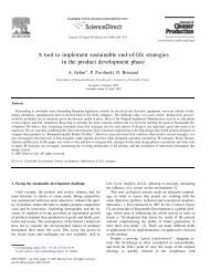
Mathematical Modeling for Reconfigurable Process PlanningA. Azab, H.A. ElMaraghy (1)Intelligent Manufacturing Systems (IMS) Centre, University of Windsor, CanadaAbstractThe paradigm shift in manufacturing systems and their increased flexibility, and changeability requirecorresponding responsiveness in support functions to achieve cost-effective adaptability. ReconfigurableProcess Planning (RPP) is an important enabler of changeability for evolving products and systems.Mathematical programming and formulation is presented, for the first time, to reconfigure process plans toaccount for changes in parts’ features beyond the scope of the original product family. Reconfiguration ofprecedence graphs to optimize the scope and cost of process plans reconfiguration is achieved byinserting/removing features iteratively using a novel 0-1 integer programming model. The proposed RPPmathematical scheme scales better with problem size compared with classical process planning models. Theformulation of the mathematical model at each iterative step of reconfiguration has been automated. Aprocess plan reconfiguration index (RI) that captures the extent of changes in the plan and their implicationshas been introduced. A prismatic benchmark and an industrial case study are used for illustration andverification. The computational behavior and advantages of the proposed model are discussed, analyzed andcompared with classical models.Keywords:Computer automated process planning, Mathematical programming, Reconfigurable process planning1 INTRODUCTIONManufacturers in the Western world are faced with morechallenges due to the fierce competition from emergingnew economic powers and open markets that areincreasingly revolving around customers needsworldwide. They must continuously develop and enhancetheir products designs and quality by applying state of theart products and system design methods and adoptingcutting edge manufacturing philosophies. Rapid evolutionof the current manufacturing systems is witnessedthrough the advent of new technologies such asChangeable and Reconfigurable Manufacturing Systems(RMS) [Koren et al., 1999].Reconfigurability aims at achieving more competitivenessby offering enablers in terms of technology and supportingbusiness paradigms [ElMaraghy, 2005]. Reconfigurationcould be achieved at the system or machine levels and itmay be soft (logical) or hard (physical) in nature. Processplanning is an important soft type enabler for suchchangeable systems. It is a critical function for theoperation planning and system design of anymanufacturing system. Variant process planningtechniques lend themselves to RMS since, like FlexibleManufacturing Systems (FMS), RMS is usually designedfor a certain part family but with wider scope. However,generative process planning systems are better able tohandle un-planned product variations. Therefore, a hybridReconfigurable Process Planning (RPP) system that isvariant in nature yet capable of generating process plansfor parts with machining features beyond those present inthe current part family’s composite part can best meet thecurrent challenges [Azab et al., 2006].In this work, a novel mathematical model for RPP isintroduced, where process plan reconfiguration takesplace by finding an optimal scheme for inserting/removingfeatures within the prescribed constraints.2 PREVIOUS WORKVery few publications have tackled the RPP problem.Zaeh et al. [2006] suggested that Agile Process Planningis useful for the production of individualized products andconstantly reconfiguring companies. ElMaraghy [2006]classified the various process planning concepts andapproaches, based on their level of granularity, degree ofautomation, and scope. The new concept of “EvolvingParts/Products Families” was introduced. The need for“Evolvable and Reconfigurable Process Plans”, which arecapable of responding efficiently to both subtle and majorchanges in “Evolving Parts/Products Families” andchangeable and Reconfigurable Manufacturing Systemswas indicated.The most relevant process planning approaches thatsupport, to varying degrees, changeable and agilemanufacturing paradigms are:2.1 Variant Process Planning SystemsRetrieval process planning is confined to changes withinthe scope of the planned family and its master compositepart. Hetem [2003] stated that the variant concept of RPPis increasingly becoming a reality in power-trainmanufacturing engineering. Feature based processtemplates may be modified to suit new designs within thefamily. Bley and Zenner [2005] proposed an integratedvariant management concept to meet the continuouslychanging needs and used features technology andgeneralized product models.2.2 Generative Process Planning SystemsIn this approach, a new process planning problem is resolvedgeneratively for every new product configuration.In most literature, a mathematical or rather a proceduralmethod is proposed and solved using either near-optimaloptimization methods or heuristics. Xu, et al. [2004]presented a clustering method for-multi part operationsplanning based on analyzing process plans forAnnals of the CIRP Vol. 56/1/2007 -467- doi:10.1016/j.cirp.2007.05.112

3. A machining feature is defined in this work as ageometrical feature that requires processing by one ormore operation.4. Sequencing is carried out on machining featurestaking the following into considerations:a) Within each feature, logical sequence of operationsis used to order the feature’s sub-operations.b) Some features are represented by more than onenode in exceptional cases due to interdependenceon precedence relationships with other features.5. The ratio of the time required to position the workpieceon a different fixture (composed mainly of unloadingthe workpiece, cleaning the setup and loading theworkpiece) to the tool changeover time is assumed tobe 2:1.The notations used are as follows: n denotes the problem size and it is the total numberof decision variables and it could also be interpretedas the total number of machining features includingthe new machining feature to-be-inserted. [C] is precedence penalty cost matrix. [S] is the setup cost matrix. {Os} is the setup cost array for original features- that isnot to include the new feature. {Tr} is the tooling right change cost array. {Tl} is the tooling left change cost array. {Ot} is the tool change cost array for original featuresnotincluding the new feature(s).The decision variables are:x i 0-1 integer variables, where i runs from 1 to n. 1 ifnew feature is inserted at position i; 0 otherwise.The position i takes the value 1 when the newfeature is inserted right before the first feature ofthe original array of operations and takes thevalue n when it is positioned right after the lastfeature of the original array, i.e. feature f n-1 (seeFigure 1).4.2 Objective Function FormulationTwo criteria are considered: 1) time for repositioning theworkpiece on different fixtures, and 2) time for toolschangeover. The objective is to minimize the non-cuttingtime. The time spent for rapid tool traverse from onefeature to the other is ignored due to its relatively minorcontribution. Also the time required for transportation ofthe workpiece between different machine tools as well asthat spent to adjust machining conditions are also ignoredsince these detailed parameters are not determined atthis macro-level. The objective function is:n n1 n n1n n nC i, jxi Si,j xiOsix i Tr iTl i xiOtixii1 j1 i1 j1 i1 i1 i1min . ( ). . ( ). . (1)The first term represents the penalty for violatingprecedence constraints. The second term represents thecost of repositioning the workpiece on the differentfixtures (i.e. setup cost as commonly referred to in theliterature). The first summation of S i,j over j represents thesetup cost associated with a new sequence, i.e. the setupcost between every pair of preceding features in thispermutation.The terms Tr i and Tl i with their summation over i from 1 ton depict the tool changeover cost. They account for thenew precedence cost due to the insertion of the newfeature between two existing features in the originalsequence- one to the right (Tr i ) and one to the left (Tl i ).Finally, the Os i and Ot i terms represent the cost incurreddue to changing the original precedence between the twofeatures that are separated by inserting the new feature,and hence, the old setup and tool costs are subtracted.4.3 Constraints FormulationThe constraints system of the RPP model isadvantageously simple and is represented by:n1i1xi 1 (2)This constraint prevents a feature from being insertedmore than once at any position.4.4 Computational ComplexityThe comparison of the computational time complexity ofthe proposed model with the classical re-planning using aTSP model raises some interesting observations. TheTSP model is a network of nodes representing differentfeatures of a part connected by arcs that represent theroutes between them. The decision variable is the valueassociated with the arc; if the value is 1 then the routerepresented by this arc is in use; it is 0 otherwise. An arcin use means that the two features are sequencedconsecutively. This model is characterized by its relativelylarge solution space (2 n , where n is the total number ofroutes) and number of complicated constraints, especiallythose to eliminate subtours. The picture is completelydifferent for the proposed RPP model. The solution spacefor inserting an m feature into an original chromosome ofsize n is 2 n-m+1 +…+2 n-1 +2 n . This could be easily simplifiedinto 2 n+1 -2 n-m+1 . Note the difference between the n of theTSP and that of the RPP models: n of TSP is the totalnumber of possible routes between the different features;however, n and m of RPP are the number of original andadded features respectively. The size of an RPPoptimization problem instance is clearly far less than itsTSP counterpart. Hence, typical industrial problems canbe easily solved for optimality using the RPP model.4.5 Demonstrative ExampleA handspike/lever [Reddy et al., 1999] is assumed to bethe new part with a new feature. It is composed of 8features (Table 1). For simplicity, the composite part isthe same part less feature B and the tapping operationsassociated with features D, E and F are disregarded.Table 1 shows the features setup and tooling data. Figure2 shows the FPGs for both the composite and the newpart. The process sequence for the composite part isobtained using the exact optimal algorithm developed in[Azab, 2003]. The obtained sequence is {A r , G, C, A f , E,D, F}. Feature A is divided into sub-features A r and A f forthe reasons explained in section 4.1 and clearly justifiedby the FPGs shown in Figure 2.-B--A-GCΦ0.05 M B MADBEF┴ Φ0.05 AFigure 2: Model of the new handspike family member,adapted from Reddy et al. [1999].The problem is formulated and solved using Xpress-MP.Feature B was inserted at position 3 in the process plansequence, i.e. x 3 = 1. The new reconfigured sequence is{A r , G, B, C, A f , E, D, F}. The penalty, setup and toolingcost matrices and vectors are given in Tables 2-13. They-A--469-

are derived from the setup/tooling information in Table 1.An element C i,j represents the penalty between a pair oftwo features; one is always being the inserted feature. Forexample Tables 2 and 3 show that there is a penalty of Mif A r is preceded by B, and 0 otherwise. For the rest of thecoefficient matrices/vectors, an element would representthe tooling or the setup cost between a pair of features.Unlike the C matrix, for the rest of the matrices thesetup/tool cost of a given features pair and its transposehave the same values since the order does not affect thetooling/setup precedence costs vector. For example inTable 12 the setup cost of having A r being preceded by Bor vice versa is the same. Note that the first and lastelements of the old setup and tooling vectors are alwayszero since if the new feature is inserted right before all thefeatures or after them, no old setup cost has to beconsidered. Also the first element of the left tooling costvector and the last element of the right tooling costelement have to be zeros because for example for the lefttooling the new feature is inserted such that the originalfeatures come to the left and hence the first decisionvariable would not be associated with any of its elements.However, note that the values of the left tooling costvector is exactly the same as the right tooling cost vectorbut shifted by one element.Feature Name Setup (Fixture) ToolingAr S1 T1C S1 T2D S2 T3E S2 T3F S2 T3G S1 T4Af S1 T5B S2 T6Table 1: Setup/Tooling data for the handspike * .*Note: B is the new feature for the new part; otherfeatures exist in both the composite and new part.0 T T T T T T 0Table 7: Filled-in old tooling cost vector0 A r B CB DB EB FB GB A F BTable 8: Tooling left changeover cost vector0 T T T T T T TTable 9: Filled-in tooling left changeover cost vectorBA r BC BD BE BF BG BA F 0Table 10: Tooling right changeover cost vectorT T T T T T T 0Table 11: Filled-in tooling right changeover cost vectorBA r A r C CD DE EF FG GA fA r B BC CD DE EF FG GA fA r C CB BD DE EF FG GA fA r C CD DB BE EF FG GA fA r C CD DE EB BF FG GA fA r C CD DE EF FB BG GA fA r C CD DE EF FG GB BA fA r C CD DE EF FG GA f A f BTable 12: Setup cost matrixS 0 S 0 0 S 0S S S 0 0 S 00 S 0 0 0 S 00 S 0 0 0 S 00 S 0 0 0 S 00 S 0 0 0 S 00 S 0 0 S S S0 S 0 0 S 0 STable 13: Filled-in setup cost matrixBA r BC BD BE BF BG BA fA r B BC BD BE BF BG BA fA r B CB BD BE BF BG BA fA r B CB DB BE BF BG BA fA r B CB DB EB BF BG BA fA r B CB DB EB FB BG BA fA r B CB DB EB FB GB BA fA r B CB DB EB FB GB A f BTable 2: Precedence penalty cost matrixDEFA f A rCGA fDEBFA rC GA fA fM 0 0 0 0 0 00 0 0 0 0 0 00 0 0 0 0 0 00 0 M 0 0 0 00 0 M M 0 0 00 0 M M M 0 00 0 M M M 0 00 0 M M M 0 MTable 3: Filled-in precedence penalty cost matrix0 A r C CD DE EF FG GA F 0Table 4: Old setup cost vector0 0 S 0 0 S 0 0Table 5: Filled-in old setup cost vector0 A r C CD DE EF FG GA F 0Table 6: Old tooling cost vectorFigure 3: Features Precedence Graphs (FPGs) for thecomposite part and new handspike.The formulation coefficient matrices/vectors are shownwith the feature pairs to illustrate the method and thenwith their corresponding values as shown in tables 2-13.S stands for Setup cost; T for Tool change cost and M isa very high positive value representing a penalty. Cells inboth the C penalty cost matrix and the S setup cost matrixare highlighted to demonstrate the repeatability of thedifferent elements. One is not required to fill in all theelements for both matrices. In fact for matrix C, only thefirst row and the diagonal are filled in and the rest issimply a repetition. The diagonal is highlighted; all theelements below the diagonal are identical and equal to itsrespective diagonal elements. All the elements above adiagonal element are the same as the cells in the matrixfirst row. As for the S matrix, there is a diagonal band witha width of two identical elements. The elements below theband are identical to their respective diagonal elements.The elements above the band are the same as those ofthe first row. Populating these matrices, althoughstraightforward, can be error prone and tedious for-470-

elatively large size problems. Therefore, the process ofgenerating the different penalty, setup and toolingcoefficient matrices has been automated using algorithmsimplemented in Matlab and fed to Xpress-MP using aninput data file.4.6 Reconfiguration Index (RI)A master process plan is reconfigured to arrive at a newplan for a new part using the proposed methodology andmathematical model. A metric is proposed to measure thepercentage of change, i.e. reconfiguration of the originalmaster process plan due to the additional insertedfeature(s). The Reconfiguration Index (RI) measures theamount of added work, time and hence cost that isneeded to reconfigure the original process plan. RIconsists of two components: changes in setups (RI s ) andchanges in tooling (RI t ). Weights are used to normalizethe index and to reflect the relative importance of itsrespective terms. Number of added setupsTotal number of setups of master plan RI .100 (3)Number of added tool changes (1 )Total number of tool changes of master planThe higher the value of RI, the more extensive is theprocess plan reconfiguration and its associated cost.5 CASE STUDY5.1 Front Engine Cover Problem DescriptionA family of engine front covers [Azab et al., 2006] is usedfor illustration. The family’s composite part is shown inFigure 4. 3D views are used as the master representationfor compactness. Sample geometric and dimensioningtolerance specifications and annotations, relevant to theapplied precedence constraints, are shown on the 3Dviews. Details of some features, their correspondingoperations, tools, and Tool Access Directions (TAD) areshown in Table 14. A three-axis horizontal ReconfigurableMachine Tool (RMT) is used for machining it, hence,three setups are required to produce the part in order toaccess the features on the front and back faces (-Z, +Z)and the side face (+X). The part is located on specificcast datum points to machine the features on the backface (+Z).Figure 4: The Front engine cover composite Part.A new member of the front cover extended/evolved familyis shown in Figure 6. The FPGs for both parts are shownin Figure 5. The new cover contains 8 features incommon with the existing composite part, but also has 7new features. The original three-axis horizontalconfiguration of the RMT would not be sufficient forproducing the new part; due to the oblique orientation offeature f17. Therefore, an extra dedicated setup or anaddition of a fourth axis to re-orient the part is required.f1FeatureIDOperationsToolIDToolsTADf1 Drilling T1 Step Drill Zf2 Drilling T4 Core Drill -Zf3 Milling T5 End Mill Zf6 Drilling T4 Core Drill Zf8 Tapping T10 M 20, Tap Xf12 Drilling T1 Step Drill ZTable 14: Sample of cover features informationf5f6f10f1f14f9f4f11f3rf16f7f2f3ff1f3rf8f17f7rf4f23f2f18f6f3fNewfeaturesf7ff5 f20 f19f21Figure 5: Feature precedence graph (FPG) of the originalcomposite and the new cylinder front cover.f22Figure 6: New member of the cylinder front covers family.5.2 RPP Formulation / Front Engine CoverFor the sake brevity, not all the formulations are shownfor the seven different iterations that were carried out. Alldetails for the first formulation are given below.1000 0 0 0 0 0 0 0 00 0 0 0 0 0 0 0 00 0 0 0 0 0 0 0 00 0 0 0 0 0 0 0 00 0 0 0 0 0 0 0 00 0 0 0 0 0 0 0 00 0 0 0 0 0 0 0 00 0 0 0 0 0 0 0 00 0 0 0 0 0 0 0 00 0 0 0 0 0 0 0 0Table 15: Penalty cost matrix, 1st iteration.2 0 2 2 2 2 0 0 22 2 2 2 2 2 0 0 20 2 2 2 2 2 0 0 20 2 2 2 2 2 0 0 20 2 2 2 0 2 0 0 20 2 2 2 0 2 0 0 20 2 2 2 2 2 2 0 20 2 2 2 2 0 2 2 20 2 2 2 2 0 0 2 20 2 2 2 2 0 0 2 2Table 16: Setup cost matrix, 1st iteration.-471-

0 0 2 2 2 2 0 0 2 0Table 17: Old setup cost vector, 1st iteration.0 1 1 1 1 1 1 1 1 0Table 18: Old tooling change cost vector, 1st iteration.0 1 1 1 1 0 1 1 1 1Table 19: Right tooling change cost vector, 1st iteration.1 1 1 1 0 1 1 1 1 0Table 20: Left tooling change cost vector, 1st iteration.6 RESULTS AND DISCUSSIONThe master macro-process plan for the composite enginecover was solved using Genetic Algorithms (GAs). Theobtained features sequence is {f13, f12, f1, f5, f6, f15, f3r,f10, f8, f4, f14, f2, f16, f11, f9, f7, f3f}. The commonfeatures {f1, f5, f6, f3r, f8, f4, f2, f7, f3f} are extracted fromthis solution by subtracting those that are not found in thenew part. Now that the initial features sequence isobtained, the RPP procedure is applied to find theoptimum insertion position for features f17- f23respectively. Formulation for the first iteration issummarized in Tables 15-20. Solutions for the seveniterations are given below.#1 {f1, f5, f6, f3r, f17, f8, f4, f2, f7r, f7f, f3f}#2 {f1, f5, f6, f3r, f17, f8, f4, f2, f7r, f18, f7f, f3f}#3 {f1, f5, f19, f6, f3r, f17, f8, f4, f2, f7r, f18, f7f, f3f}#4 {f1, f5, f20, f19, f6, f3r, f17, f8, f4, f2, f7r, f18, f7f, f3f}#5 {f1, f5, f20, f19, f6, f3r, f17, f8, f4, f2, f7r, f18, f7f, f21, f3f}#6 {f1, f5, f20, f19, f6, f3r, f17, f8, f4, f2, f7r, f18, f7f, f21, f22, f3f}#7 {f1, f5, f20, f19, f6, f23, f3r, f17, f8, f4, f2, f7r, f18, f7f, f21,f22, f3f}The RI for the new plan is 89.8 % indicating that themaster plan was significantly reconfigured. The processsequence for the same new part was obtained using GAswith a 17% improvement in the value of the objectivefunction. This is expected since the re-planning approachsolves the whole global sequencing problem, while theproposed RPP algorithm limits reconfiguration to a subsetof the total solution space. This is an advantage in agilemanufacturing environments where products evolve andare customized frequently. The RPP methodology offers aquick, feasible and optimal solution albeit not the exactglobal optimum.7 CONCLUSIONSA novel semi-generative mathematical model forreconfiguring macro-level process plans has beenpresented. It supports evolvable part families, which arebecoming a reality, due to the current challenges ofunpredictable customer-centered markets and emergenceof new reconfigurable and changeable manufacturingequipment and agile business paradigms. The presentedRPP model is compared with the classical TSP replanningapproach. Although both the RPP and TSP replanningmodels are NP-complete, the RPP modelprovides much smaller solution space and lesscomplicated number of constraints; hence, it iscomputationally more tractable. The problem formulationwas automated. A process plan reconfiguration index (RI)has been proposed. It can be used for choosing amongalternate sequences with substantially similar total cost byopting for the one that causes the least changes on theshop floor, which saves other indirect costs such as thoserelated to errors and quality issues due to changes. Oneof the main contributions is the development of a newmathematical model for solving the classical problem ofprocess planning and sequencing throughreconfiguration. The developed methods are applicable inother fields of science and engineering where classicaloptimal sequencing problems exist.8 REFERENCES[1] Azab, A., Perusi, G., ElMaraghy, H. and Urbanic J.,2006, Semi-Generative Macro-Process Planning forReconfigurable Manufacturing, Proc. CIRP Int. DigitalEnterprise Tech. (DET) conf., Setubal, Portugal.[2] Azab, A., 2003, Optimal Sequencing of MachiningOperations, M.Sc. thesis, Cairo University.[3] Bhaskara Reddy S. V., Shunmugam, M.S. andNarendran, T.T., 1999, Operation Sequencing inCAPP Using Genetic Algorithms, IJPR, 37: 1063-1074.[4] BLEY H. and ZENNER, C., 2005, Feature-basedPlanning of Reconfigurable Manufacturing Systemsby a Variant Management Approach, CIRP 3rd Int.lConf. on RMS, Ann Arbor, MI.[5] ElMaraghy, H.A., 2005, Flexible and ReconfigurableManufacturing Systems Paradigms, Special Issue ofthe Int.l J. of Flexible Manuf. Sys. (IJFMS),(http://dx.doi.org/10.1007/s10696-006-9028-7), 17/4 :261-276.[6] ElMaraghy, H.A., 2006, Reconfigurable ProcessPlans for Responsive Manufacturing Systems,” Proc.CIRP Int.l Digital Enterprise Tech. (DET) Conf.,Setubal, Portugal, (keynote paper).[7] Halevi, G. and Weill, R. D., 1995, Principles ofProcess Planning: Chapman & Hall.[8] HETEM, V., 2003, Variant Process Planning, a Basisfor Reconfigurable Manufacturing Systems, CIRP2nd Int.l Conf. on RMS, Ann Arbor, MI.[9] Koren, Y., Heisel, U., Jovane, F., Moriwaki, T.,Pritschow, G., Van Brussel, H., Ulsoy, A.G., 1999,Reconfigurable Manufacturing Systems, Annals ofthe CIRP, 48/2: 527-540, (keynote paper).[10] Koulamas, C., 1993, Operation Sequencing andMachining Economics, IJPR, 31 : 957- 975.[11] Lin, C.-J. and Wang, H.-P., 1993, Optimal OperationPlanning and Sequencing: Minimization of ToolChangeovers, IJPR, 31 : 311-324.[12] Lin, C., Lin, S.-Y., and Diganta, D., 1998, AnIntegrated Approach to Determining the Sequence ofMachining Operations for Prismatic Parts withInteracting Features, J. Materials Proc. Tech., 73 :234-250.[13] Shabaka, A.I., ElMaraghy, H.A., 2006, Generation ofMachine Configurations Based on Product Features,Int. J. Comp. Integrated Manuf., DOI:10.1080/09511920600740627, Paper Number:TCIM-2005_IJCIM-0020.[14] Zaeh, M. F., Rudolf, H. and Moeller, N., 2005, AgileProcess Planning Considering a Continuous FactoryReconfiguration, Proc. CIRP 3rd Int.l Conf. on RMS,Ann Arbor, MI.[15] XU, H., TANG, R.-Z. and CHENG, Y.-D., 2004,Study Of Process Planning Techniques ForReconfigurable Machine Tool Design, J. of ZhejiangUniversity, 38 :1496-1501.-472-