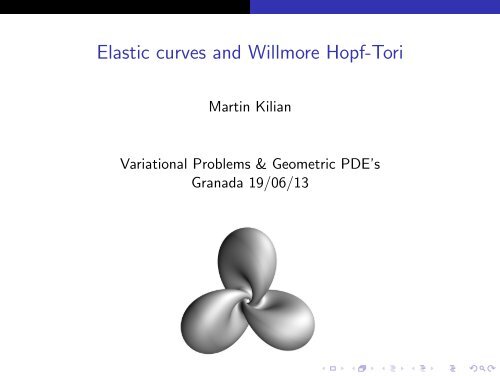
Elastic curves and Willmore Hopf-Tori
Elastic curves and Willmore Hopf-Tori
Elastic curves and Willmore Hopf-Tori

You also want an ePaper? Increase the reach of your titles
YUMPU automatically turns print PDFs into web optimized ePapers that Google loves.
A brief history◮ 1691 J. Bernoulli: first characterization of planar elastica◮ 1742 D. Bernoulli: proposed variational techniques◮ 1744 Euler: characterization using variational methods◮ 1984 Langer-Singer: classified elastica on 2-sphere◮ 1985 Pinkall: connection between elastica <strong>and</strong> <strong>Willmore</strong> tori◮ 1991 Goldstein-Petrich: relationship to mKdV◮ 2003/04 Arroyo-Garay-Mencia: closed elastica <strong>and</strong>generalizations◮ 2008 Bohle-Peters-Pinkall: constrained elastica, <strong>and</strong>constrained <strong>Willmore</strong> <strong>Hopf</strong>-tori◮ 2012 L.Heller, J.Zentgraf: PhD theses on constrained<strong>Willmore</strong> <strong>Hopf</strong>-tori etc.
Outline of talk:◮ Joint work with F. Pedit <strong>and</strong> N. Schmitt◮ Finite type <strong>curves</strong> on S 2◮ Polynomial Killing fields <strong>and</strong> spectral <strong>curves</strong>◮ Whitham deformation◮ Constrained elastic <strong>curves</strong>◮ Moduli space of constrained <strong>Willmore</strong> <strong>Hopf</strong>-tori
◮ If h : S 3 → S 2 is the <strong>Hopf</strong>-fibration, then h −1 (γ) for a closedcurve γ : R → S 2 is called a <strong>Hopf</strong>-torus. The curve is calledits profile curve◮ A <strong>Hopf</strong>-torus is a constrained <strong>Willmore</strong> <strong>Hopf</strong>-torus iff itsprofile curve is a closed constrained elastic curve (area <strong>and</strong>length constraint). Its geodesic curvature satisfiesκ ′2 + 1 4 κ4 + a κ 2 + b κ + c = 0 .◮ When b = 0 we speak of elastic <strong>curves</strong> (area constraint).◮ The torus is a <strong>Willmore</strong> <strong>Hopf</strong>-torus iff the profile curve is aclosed free elastic curve (no constraint). Its geodesiccurvature satisfiesκ ′2 + 1 4 κ4 + 1 2 κ2 + c = 0 .
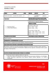
Constrained <strong>Willmore</strong> <strong>Hopf</strong>-toriFigure: A sequence of 3-lobed constrained <strong>Willmore</strong> <strong>Hopf</strong>-tori, starting atthe Clifford torus, <strong>and</strong> ending at a <strong>Willmore</strong> <strong>Hopf</strong>-torus
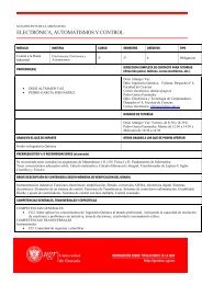
Figure: A deformation through constrained elastic <strong>curves</strong>, starting near a1-wrapped equator <strong>and</strong> ending near a 5-wrapped equator
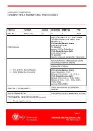
TheoremThe <strong>Willmore</strong> energy along each deformation family containing a<strong>Willmore</strong> <strong>Hopf</strong>-torus attains its maximum at this torus. The2-lobed <strong>Willmore</strong> <strong>Hopf</strong>-torus has the least energy among the<strong>Willmore</strong> <strong>Hopf</strong>-tori.Figure:The 2-lobed <strong>Willmore</strong> torus, <strong>and</strong> its free elastic profile curve.
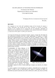
Finite type <strong>curves</strong> in S 2Curves in S 2Let γ : R → S 2 be a smooth immersed arc-length parametrizedcurve with geodesic curvature κ. The frame G : R → SO 3 of γwith columnsG = (γ, γ ′ , γ × γ ′ )satisfies⎛0 −1⎞0G ′ = G ⎝1 0 −κ⎠ .0 κ 0Here prime denotes differentiation with respect to arc-length.
Finite type <strong>curves</strong> in S 2mKdV hierarchyThe mKdV hierarchy is an infinite hierarchy of evolution equationswith first three equations˙κ = −κ ′˙κ = −k ′′′ − 3 2 κ2 κ ′˙κ = −k ′′′′′ − 15 8 κ4 κ ′ − 5 2 κ2 κ ′′′ − 10κκ ′ κ ′′.A curve is called of finite type if κ is stationary under all but fintelymany of the flows in this hierarchy.
Finite type <strong>curves</strong> in S 2ReconstructionVia the double cover SU 2 → SO 3 the extended frame equation canbe written as( )F λ ′ = F iλ κλwhere λ ∈ R .−κ −iλThe associate family of <strong>curves</strong> R → SU 2 ∩ R 3 ∼ = S 2 given byγ λ = F λ F −1−λhas geodesic curvature λ −1 κ, <strong>and</strong> constant speed |λ|.Call the evaluation points the sym points (w.l.o.g. take λ = 1).
Polynomial Killing fields <strong>and</strong> spectral curvePolynomial Killing fieldsPolynomial Killing fieldsA polynomial Killing field of a curve on S 2 is a polynomialX =d∑X k λ k where X d =k=0( )i 00 −iwith X k : R → su 2 smooth that satisfies a Lax equationX ′ = 1 2 [X, V (X)] with V (X) := X d−1 + X d λ ,<strong>and</strong> is twisted (or anti-twisted), so thatX(−λ) = ± ( ) (0 1−1 0 X(λ) 0 1)−1 0 .
Polynomial Killing fields <strong>and</strong> spectral curvePolynomial Killing fieldsFinite type <strong>curves</strong>A finite type curve R → S 2 is one whose extended frame satisfiesF ′ λ = 1 2 F λ V (X) , F λ (0) = 1for some polynomial Killing field X.Let X(0) = X 0 . ThenF −1λ X 0F λ = X ,so det X = det X 0 is independent of arc-length. By thetwistedness condition det X is an even polynomial.
Polynomial Killing fields <strong>and</strong> spectral curveSpectral curveSpectral curve◮ Suppose X is a polynomial Killing field of degree d, <strong>and</strong>X 0 = X(0).◮ Since X 0 ∈ su 2 conclude that det X is a real, even polynomialof degree 2d.◮ Assume all the roots of det X are simple.◮ The spectral curve Σ of X is the hyperelliptic curve over Cwith branchpoints only at the roots of det X. It is a compactRiemann surface of genus g = d − 1.◮ The genus g of Σ is called spectral genus.
Polynomial Killing fields <strong>and</strong> spectral curveSpectral curveClosing conditionsLet X be a periodic polynomial Killing field with period ρ, <strong>and</strong>extended frame F λ . Then the corresponding curve is closed if <strong>and</strong>only if the monodromy M λ = F λ (ρ) satisfiesM 1 = M −1 = 1 or M 1 = M −1 = −1 .From F −1λX 0F λ = X <strong>and</strong> X 0 = X(ρ) it follows that[X 0 , M λ ] = 0 .An eigenvalue µ of M λ is a meromorphic function on Σ whose onlypoles are simple poles over the two points ∞ ± .
Whitham deformationPolynomials A, B <strong>and</strong> CWhitham deformationHence d log µ is an abelian differential of the 2 nd kind on Σ, so ofthe formd log µ = √ B dλAwhere A = det X <strong>and</strong> λ ↦→ B(λ) is a real polynomial of degreed = g + 1.Suppose A <strong>and</strong> B depend on an additional parameter t ∈ R. Canwriteddt log µ = √ C Awhere λ ↦→ C(λ) is a polynomial of degree at most g.
Whitham deformationPolynomials A, B <strong>and</strong> CThe deformation in the parameter t is subject to the integrabilityconditiond 2dλ dt log µ =d2dt dλ log µ ,or equivalently in terms of the polynomials A, B <strong>and</strong> C that2 A Ḃ − ˙ A B = 2 AC ′ − A ′ C . (3.1)The variables in the flow are the 2g + 2 coefficients of A, <strong>and</strong> theg + 1 coefficients of B. The g + 1 coefficients of C can be chosenfreely.
Whitham deformationPolynomials A, B <strong>and</strong> CTo preserve closing conditions µ(λ) = µ(−λ) = ±1 at λ = 1during the deformation, also require(ddt log µ∣ ∣λ=±1= ( ddλ log µ) ˙λ)∣+ d dt log µ ∣∣λ=±1= 0 ,or equivalently˙λ ∣ = − C λ=±1 B ∣ . (3.2)λ=±1Thus we may fix the sym points at λ = ±1 during the flow bypicking C to have fixed zeroes there. Equations (3.1) <strong>and</strong> (3.2)define a meromorphic vector field on the parameter space ofcoefficients of A <strong>and</strong> B.
Whitham deformationIncreasing the spectral genusIncreasing the spectral genusLemmaLet X be a polynomial Killing field. Then (λ 2 − a 2 ) X for a ∈ R isa polynomial Killing field, <strong>and</strong> both induce the same curve.Opening double points:◮ Suppose a ∈ R is a double point on Σ.◮ Then µ(a) = ±1 <strong>and</strong> writed log µ =(λ2 − a 2 ) B(λ 2 − a 2 ) √ A dλ .◮ Now can pick initial condition for the flow at t = 0 such thatwhen t > 0 the roots ±a move vertically off the real axis.
Whitham deformationExampleCirclesThe simplest polynomial Killing field is( )iλ κX =−κ −iλwith κ ∈ R constant. The corresponding <strong>curves</strong> are circles with(geodesic) curvature κ, <strong>and</strong> the branchpoints of the spectral curveare located at ±iκ. Since log µ = πi√λ 2 + κ 2 , doublepoints area ∈ R with a 2 + κ 2 ∈ Z 2 .Figure:The spectral curve of a bifurcating circle.
Whitham deformationExampleThe branchpoints of the spectral curve of an elastic curve are theroots of the real even quartic polynomialm 4 + m 2 λ 2 + λ 4 .With discriminant ∆ = 1 4 m 2 − m 4 , away from degeneratesituations, there are two caseswave-like if ∆ < 0: distinct branchpoints ±p 1 , ±p 2 with p 2 = ¯p 1orbit-like if ∆ > 0: distinct branchpoints on iR × .In the case ∆ = 0 the spectral curve is singular.Figure: Spectral <strong>curves</strong> of wave-like <strong>and</strong> orbit-like elastic <strong>curves</strong>.
Whitham deformation Flow of elastic <strong>curves</strong> in S 2Flowing off a great circle by opening up a pair of branchpointsincreases the spectral genus from g = 0 to g = 1. The flowthrough closed elastic <strong>curves</strong> of spectral genus g = 1 are given byṗ 1 = (1 − p 2 1)(p 2 + p 1 β) ,ṗ 2 = (1 − p 2 2)(p 1 + p 2 β) .Qualitative analysis of these equations yield a picture of the modulispace of closed elastic <strong>curves</strong> on S 2 .
Whitham deformation Flow of elastic <strong>curves</strong> in S 2Properties of elastic <strong>curves</strong>◮ Wave-like elastica bifurcate off great circles.◮ Free elastic <strong>curves</strong> (no area or length constraint) are wave-like.◮ Orbit-like elastica bifurcate off non-great, at least twicewrapped circles. They are never embedded, <strong>and</strong> always end ina singular limit.◮ Some wave-like families deform between ω 1 –wrapped <strong>and</strong>ω 2 –wrapped equators. Denote the the lobe number by l.Then for l/ω 1 ∈ (1/2, 1) ∩ Q haveω 1 + ω 2 = 2l .◮ Free elastica are only contained in families withl/ω 1 ∈ (1/2, 1/ √ 2).
Whitham deformation The moduli space of closed wavelike elastic <strong>curves</strong> in S 2 .Figure: Closed wave-like elastica lie on a discrete dense set of <strong>curves</strong>. Theposition of the branchpoint in the first quadrant is shown. All1-parameter family of closed wave-like elastica start at a multiwrappedequator (along the real axis). The semicircle-like <strong>curves</strong> represent familieswhich end at multiwrapped equators, those to the left of the thick lineend in a singular limit. The thick curve marks the boundary betweenthese two types. The dashed curve represents the free elastica.
Whitham deformation The moduli space of closed wavelike elastic <strong>curves</strong> in S 2 .Figure:Orbit-like example with orbit-like elastic profile curve.
Whitham deformation The moduli space of closed wavelike elastic <strong>curves</strong> in S 2 .Constrained elastica on S 2 arise from anti-twisted polynomialKilling fields of degree 3:( )iA BX =−B ∗ −iAwhereA = 1 2 (m 2 − κ 2 )λ + λ 3B = −(κ ′′ + 1 2 κ3 − 1 2 m 2κ) + iκ ′ λ + κλ 2 .The branchpoints of the spectral curve are the zeros ofwhere the curvature κ satisfiesdet X = m 6 + m 4 λ 2 + m 2 λ 4 + λ 6κ ′ 2 +14 κ4 − 1 2 m 2κ 2 + 2 √ m 6 κ + 1 4 m2 2 − m 4 = 0 .
Whitham deformation The moduli space of closed wavelike elastic <strong>curves</strong> in S 2 .Assuming that none of the zeros of det X are real, three classes of<strong>curves</strong> in S 2 with curvature κ can be distinguished:◮ constrained elastic: area <strong>and</strong> length constraint. no conditions;◮ elastic: area constraint, but no length constraint, m 6 = 0;◮ free elastic: no area or length constraint, m 6 = 0 <strong>and</strong>m 2 = −1.Figure: Spectral <strong>curves</strong> of wave-like <strong>and</strong> orbit-like constrained elastica.
Moduli space of constrained elasticaConstrained elastica all arise from a simple ’translational’ Whithamflow of elastica.TheoremThe moduli space of closed constrained elastica is the cartesianproduct of the 1-dimensional moduli space of closed elastica withthe half-open interval [0, 1).CorollaryThe moduli space of closed constrained elastica has two connectedcomponents, one for each homotopy type.
Moduli space of constrained elasticaLemmaThe conformal type of a constrained <strong>Willmore</strong> <strong>Hopf</strong>-torus isτ = A 4π + iL { ω4π = 2 + iL4πfor wave-like ,ω−lfor orbit-like2+ iL4πProof.Computing A using Gauss-Bonnet givesA = 2πω − l∫ ρwhere ρ is the period of κ. A computation gives∫ ρ{ 0 for wave-like ,κ =2π for orbit-like00κ
Moduli space of constrained elasticaTheoremAmongst the constrained <strong>Willmore</strong> <strong>Hopf</strong>-tori with conformal typenear the Clifford torus, the 2-lobed constrained <strong>Willmore</strong> <strong>Hopf</strong>-torihave the least <strong>Willmore</strong> energy amongst the constrained <strong>Willmore</strong><strong>Hopf</strong>-tori.
Moduli space of constrained elasticaFigure: Spectral genus g = 2 constrained wave-like elastic profile curve,<strong>and</strong> corresponding constrained <strong>Willmore</strong>-<strong>Hopf</strong>-torus.
Moduli space of constrained elasticaFigure: Nonembedded example. Spectral genus g = 2 constrainedwave-like elastic profile curve, <strong>and</strong> corresponding constrained<strong>Willmore</strong>-<strong>Hopf</strong>-torus.
Moduli space of constrained elasticaFigure: <strong>Willmore</strong> <strong>Hopf</strong>-torus with a singular spectral curve. The profilecurve is a dressed circle.