Evolution of the Whitham zone in the Korteweg-de Vries theory

EVOLUTION OF A WHITHAM ZONE INKORTEWEG–DE VRIES THEORYV. V. AVILOV AND ACADEMICIAN S. P. NOVIKOVWe consider the analogy of shock waves in KdV theory. It is well known (see[1], pp. 261–263) that the analogy of a shock front, for instance, in a collisionlessplasma described by the KdV equation, has an oscillation zone. This zone is in theframework of the averaging method described by a set of Whitham equations [2] forthree slowly varying quantities which in a given cycle of problems were first usedby Gurevich and Pitaevskii [3]. These authors studied exact self-similar solutionsof the Whitham equations on the basis of which they reached conclusions aboutthe asymptotic behavior of the oscillation zone as t → +∞.The aim of the present paper is a correct mathematical statement of the problemof the evolution of the oscillation (Whitham) zone for arbitrary boundary conditionsin the framework of the theory of sets of first order equations. This allows us, inparticular, to state and solve numerically the problem about the realizability of theself-similar regimes found in [3] as asymptotic regimes for a wide class of initialconditions as t → −∞.The KdV equation has the form u t + uu x + u xxx = 0. Averaging it against thebackground of a set of periodic cnoidal waves[ ( a) ]1/2(1) u(x, t) = 2as −2 dn 2 (x − V t), s6s 2 + γwith slowly varying parameters a, s, and γ leads to Whitham equations of the form(2) r αt = v α (a, s, γ)r αx , α = 1, 2, 3,where(3) a = r 2 − r 1 , s 2 = r 2 − r 1r 3 − r 1, γ = r 2 + r 1 − r 3 ;the equations for v α are given in [1], p. 264. Here v 3 v 2 v 1 , r 3 r 2 r 1 . Ifr 2 = r 3 , the solution (1) describes a soliton; if r 2 = r 1 , (1) is a constant.According to the physical representations worked out in [3], the oscillation zonein the problems studied extend over the entire allowable range of variation of theparameters r α ; i.e., at any time t it is determined in the region (4), which is notknown beforehand,(4) x − (t) x x + (t)where(5)r 1 → r 2 ,r 2 → r 3 ,x → x − (t),x → x + (t).Date: Submitted April 9, 1986.Dokl. Akad. Nauk SSSR 294, 325–329 (May 1987). Translated by D. ter Haar.1

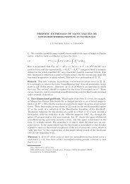
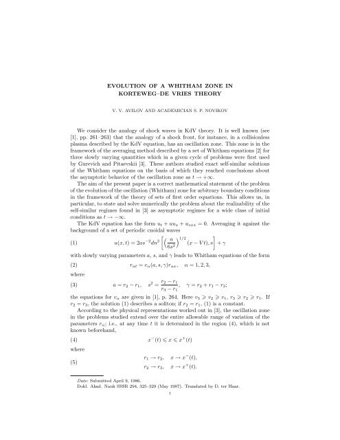
2 V. V. AVILOV AND ACADEMICIAN S. P. NOVIKOVFigure 1. Evolution of the single-valued function l(z, t) =t −1/2 r(z, t) (z = xt −3/2 ) of problem 2. The initial condition (t = 1)in the oscillation zone corresponds to a perturbation of the selfsimilarsolution; at t = 2 this distortion is appreciably diminished.The self-similar solution is indicated by dots.Outside the range (4) there are no oscillations and the functions r α (x, t) are notdefined; at the boundary of (4) the solution of Eq. (2) must be joined continuouslyto the solution of the Hopf equation u t + uu x = 0, obtained from the KdV bydropping the dispersion term, where u(x, t) is determined outside the zone (4):(6)u(x − (t), t) = r 3 (x − (t), t),u(x + (t), t) = r 1 (x + (t), t).It follows from (5) and (6) that the solution on the whole x axis is described bythe continuous function r(x, t) which is three-valued in the oscillation region (4),r = (r 1 , r 2 , r 3 ), and single-valued outside that region, r = u(x, t) (see Fig. 1).Problem. Give the mathematically correct statement of the Cauchy problem formultiple-valued functions r(x, t) which allows us to study the temporal evolutionof the oscillation zone (4).For a more complete and rigorous study the basis of such a statement must followof course from the exact KdV theory. We have, however, deliberately restricted thediscussion to the theory of first-order systems which may have a broader meaningthan the KdV theory.

EVOLUTION OF A WHITHAM ZONE IN KORTEWEG–DE VRIES THEORY 3Hydrodynamic systems without dissipation have the form(7) u α t = v α β (u)u β x,where u α (x, t) is a vector function, α = 1, 2, . . . , k. The form of (7) is conservedunder nonlinear substitution of u(w). If the matrix vβ α (u) is diagonal, the fieldsu α are called Riemann invariants. For instance, for Whitham’s system (2), k = 3,the quantities u α = r α are the Riemann invariants of (2). Recently, a theory ofHamiltonian systems of the form (7) and of the Poisson brackets connected withthem has been developed [4]. One of the authors of that paper hypothesized thata system of the form (7) is integrate if, first, it is Hamiltonian and, secondly, ithas Riemann invariants. In some sense, this hypothesis was proved in [5]. Theprocedure of [5] allows us to find some exact (“on average finite-zoned”) solutionswhich have as yet not been studied. The theorem following from [5] about thecomplete integrability of Whitham’s system (2) is of a formal, local nature. Itsapplicability to a particular global class of functions r α (x, t) has not been studied.Even more questionable is the applicability of this statement to the physicallyinteresting class described above, where the Whitham equation acts only in thefinite range (4) and is joined on the boundary to the solution of the trivial Hopfequation; the range (4) changes here with time in a way not known as yet.The system (2) possesses self-similar solutions of the form (8) with arbitraryexponent γ:(8) r α (x, t) = t γ l α (xt −1−γ ) = t γ l α (z).An important role below is played by the solution for γ = 1/2 found in [3] (see [1],pp. 280–284). Let z = xt −3/2 . Outside the zone (4) we have u(x, t) = t 1/2 θ(z),where z = θ − θ 3 . At the edges of (4), where x = x ± (t), all l ± α can be expressed interms of z ± from the conditions of continuity and constancy of the zone (4) in theself-similar variable z (see [1], p. 281).Such a solution exists and is unique, if l 3 > 0, l 1 < 0, and all l α are continuousalong with their first derivatives in the region z − < z < z + . At the point z 0 , wherel 2 (z 0 ) = 0, the second derivatives apparently are no longer continuous. Calculationsshow that(9) z − ≈ −1.141, z + ≈ 0.117, z 0 ≈ −1.11.We now turn to our problem. The class of multiple-valued continuous functionsr(x, t) must satisfy conditions (4)–(6). Moreover, these functions must be smoothclass C 1 functions outside the points x ± (t). They should be assumed to be smootheroutside zone (4). In the vicinity of the points on the curves x ± (t), the hypothesisof single-valuedness and of smoothness of the inverse function must be satisfied.This means that for any fixed t 1 the behavior of the quantity r α as x → x ± (t)is determined from Eqs. (10)–(13) at the given time t:(10)(11)Here we have(12)(13)x ′′ = (a + + b + (r − r + ))f(1 − s 2 ) + O(r − r + ) 3 ,x ′′ = x − x + 0, f(y) = y 2 [log(16/|y|) + 1/2];x ′ = a − (r − r − ) 2 + b − (r − r − ) 3 + o(r − r − ) 3 , x ′ = x − x − 0.dx + /dt = v + 2 = v+ 3 , dr+ /dt = −|r + 3 − r+ 1 |2 /(12a + ),dx − /dt = v − 1 = v− 2 , dr− /dt = −1/(2a − ).

4 V. V. AVILOV AND ACADEMICIAN S. P. NOVIKOVIf these conditions are satisfied, we call a multiple-valued function admissible at thegiven time t.Assertion. The Whitham equation, together with the Hopf equation, determinesuniquely the temporal evolution of the admissible multiple-valued functions r(x, t).Although there is no mathematically rigorous proof of this assertion, the presentauthors have constructed a numerical realization of this evolution applicable to twofunctional classes (boundary conditions) corresponding to two physical problems(see [1]).Problem 1. Decay of an initial discontinuity for the KdV. Here we haver(x, t) → 1,r(x, t) → 0,x → −∞,x → +∞.Problem 2. Dispersive analog of a shock front. Here the boundary conditions arer(x, t) − u 0 (x, y) → 0, |x| → ∞, x = u 0 t − u 3 0.In each problem we assume that the rate at which the limit is reached as |x| → ∞is sufficiently fast (exponential).Using (2), we carry out the numerical calculation by the characteristics methodoutside small regions near the points x ± (t). In the vicinity of these points thequantity r(x, t) was interpolated by Eqs. (10)–(13), where a ± (t) and b ± (t) weredetermined by joining up with the numerical solution. This enabled us to constructin each step in time the extension of the oscillation zone (4), since the derivativesẋ ± (t) and ṙ ± (t) are known. Along the line x − (t) the characteristics for r 1 and r 2are tangent and along x + (t) the characteristics for r 2 and r 3 are tangent. Theseare the singular lines: the characteristic r 1 reaches the line x − (t), touches it, andthen leaves it as the characteristic r 2 . In exactly the same way, the characteristicr 3 arrives along x + (t), touches the line x + (t), and then leaves as r 2 in the regionof the (x, t)-plane inside the curves [x + (t), x − (t)]. At each step in time around theboundaries there is a transition of one characteristic into another. In the numericalcalculation the characteristics themselves are not calculated in small regions aroundthe curves x ± (t).As boundary conditions at t = 1 for problem 2 we introduced various admissibleperturbations of the self-similar Gurevich–Pitaevskii regime (see above).The conclusions are the following: any admissible initial condition r(x, t), whichis sufficiently C 1 -close to the self-similar solution of problem 2 (see above), evolvesan infinite time without the appearance of any singularities (see Fig. 1) and ast → ∞ the functions l α (z, t) tend to the self-similar solution (8), where r α (x, t) =t 1/2 l α (z, t). There exists a finite threshold – the degree of remoteness of the initialperturbation from the self-similar solution – after which the evolution may be(and sometimes is) such that there appears the usual hydrodynamic steepening andafterwards the inversion of the front for r α . We do not know the numerical characteristicsof this threshold. In order that the evolution of r(x, t) be extended over aninfinite time as t → +∞, it is necessary (although not sufficient) that each singlevaluedcontinuous branch of the function r(x, t) be a monotonic function of x attime t. This statement is correct in all problems considered by us, as the numericalexperiment shows. Under the same necessary condition in problem 1, a wide classof admissible (although not all) initial conditions in the evolution process tend to

EVOLUTION OF A WHITHAM ZONE IN KORTEWEG–DE VRIES THEORY 5Figure 2. Evolution of the single-valued function r(z, t) (z =xt −1 ) of problem 1. The initial condition (t = 1) inside the oscillationzone corresponds to the self-similar solution of problem 2and outside this zone tends to a constant.a regime which is self-similar with exponent γ = 0, where z = xt −1 , r 1 → const,r 3 → const, and v 2 → z. This limiting regime is described in [1], pp. 268–270. Byitself it is not contained among the admissible functions, but is found to be a limit(see Fig. 2).From a methodological point of view, it is useful also to consider the case (problem3) when x + = +∞, x − = −∞, and r α (x, t) → r α ± as x → ±∞, wherer1 − = r− 2 < r− 3 , r+ 2 = r+ 3 > r+ 1 (infinite oscillation zone).Numerical calculations show that in order that the evolution does not for allt → +∞ lead to the usual hydrodynamic inversion of the front (i.e., in order that|r αx | be finite for all α), it is necessary and sufficient that at the initial time t = 1the condition for a monotonic increase of r α (x, t) is satisfied:(14) r αx 0, −∞ < x < +∞.If r 1 + < r− 3 there is a finite range of the self-similar z = xt−1 , where the solutiontends, as t → ∞, to the self-similar solution of problem 1: r 3 = r3 − , r 1 = r 1 + , v 2 = z(see Fig. 3). Hence it follows that the condition that there be no singularities inthe evolution process can in principle be formulated only in terms of the Riemanninvariants r α . It cannot be expressed in terms of the physical characteristics ofthe initial condition – such as the average velocity ū, the quantities u min and u max(see [1], p. 264), the average momentum density ¯p = u 2 , and the average energy ¯ε,

6 V. V. AVILOV AND ACADEMICIAN S. P. NOVIKOVFigure 3. Evolution of the infinite oscillation zone of problem 3.The functions r α (z, t) (z = xt −1 ), α = 1, 2, 3, at the initial timet = 1 are shown by dots, the full drawn lines correspond to t = 11.whose graphs may appear to be physically meaningful both when (14) is satisfiedand when it is violated.References[1] S. P. Novikov (ed.), Theory of Solitons, Consultants Bureau, New York.[2] G. B. Whitham, Proc. R. Soc. A283, 238 (1965).[3] A. V. Gurevich and L. P. Pitaevskii, Zh. Eksp. Teor. Fiz. 65, 590 (1973) [Sov. Phys. JETP38, 291 (1974)].[4] B. A. Dubrovin and S. P. Novikov. Dokl. Akad. Nauk SSSR 270, 781 (1984).[5] S. P. Tsarev, Dokl. Akad. Nauk SSSR 282, 280 (1985).L.D. Landau Institute of Theoretical Physics, Academy of Sciences of the USSR,Moscow