LEP 4.4.06 -01 RLC Circuit - Phywe Systeme GmbH

RLC Circuit 

LEP 

4.4.06 

-01 

Related topics 

Kirchhoff’s laws , series and parallel tuned circuit, resistance, capacitance, inductance, phase displacement, 

𝑄-factor, band-width, loss resistance, damping 

Principle 

The current and voltage of parallel and series-tuned circuits are investigated as a function of frequency. 

𝑄-factor and band-width of the resonance curves are determined. 

Material 

1 Coil, 300 turns 06513-01 

1 PEK capacitor (case 2) 1.0 µF/250V 39113-01 

1 PEK capacitor (case 1) 0.1 µF/250V 39105-18 

1 PEK carbon resistor 1 W 5% 47 Ω 

39104-62 


39104-63 


39104-15 


39104-19 

1 Connection box 

06030-23 

1 Connection plug 

39170-00 

1 Multimeter 07128-00 

1 Digital function generator 13654-99 

3 Connecting cord, l = 250 mm, red 07360-01 

3 Connecting cord, l = 250 mm, blue 07360-04 

1 Connecting cord, l = 500 mm, red 07361-01 

1 Connecting cord, l = 500 mm, blue 07631-04 

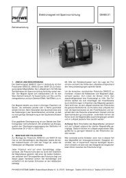
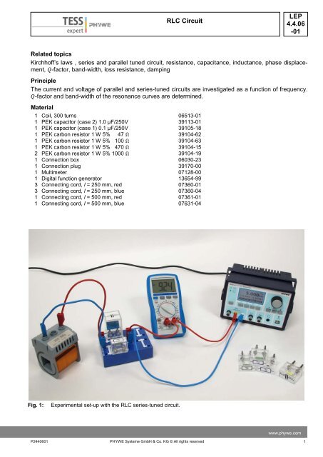
Fig. 1: Experimental set-up with the RLC series-tuned circuit. 

www.phywe.com 

P2440601 PHYWE Systeme GmbH & Co. KG © All rights reserved 1

TEP 




Tasks 

Analyze the frequency performance of an 

1. series-tuned circuit for 

a. voltage resonance with 𝑅 𝑑 = 0 Ω. 

b. current resonance with 𝑅 𝑑 = 0 Ω, 47 Ω, 100 Ω. 

2. parallel-tuned circuit for 

a. current resonance with 𝑅 𝑑 = ∞. 

b. voltage resonance with 𝑅 𝑑 = 470 Ω, 1000 Ω, ∞. 

Set-up 

The experimental set-up is shown in Fig. 1. 

For the digital function generator select following settings: 

• DC-offset: ± 0 V 

• Amplitude: 3 to 4 V 

• Frequency: 0 - 30 kHz 

• Mode: sinusoidal 

None of the settings should be changed during the 

experiment. 

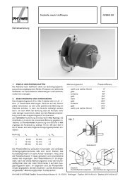
The circuit diagram for the series-tuned circuit is 

shown in Fig. 2, where 𝑅 𝑑 denotes the damping resistance. 

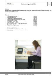
The equivalent diagram for the parallel-tuned 

circuit is shown in Fig. 3. A 1 kΩ resistor 𝑅 𝑘 is used 

for coupling the tuned circuit to the digital function 

generator. 

Fig. 2: Equivalent diagram for the series-tuned circuit. 

Procedure 

The multimeter must be set to AC mode. For measuring 

the voltage select the range up to 2 V. The 

range for the current should be 20 mA. In some 

cases it may be necessary to change the range to 

200 mA. 

In order to evaluate the quality of the resonance 

curves, the frequency generator’s internal resistance 

𝑅 𝑖 and the circuits’ loss resistances 𝑅 𝑣 have to 

be determined. To calculate the internal resistance 

of the function generator measure current and terminal 

voltage in the series-tuned circuit at the frequency 

of 0 Hz. For computing the loss resistances 

in both circuits measuring current and voltage at the 

resonance point is needed. In the case of the parallel-tuned 

circuit, the capacitors loss resistance can be ignored, as it amounts to several hundred MΩ . 

Fig. 3: Equivalent diagram for the parallel-tuned circuit. 

Task 1: 

a) To record the voltage resonance curve for the series-tuned circuit, the voltage across the tuned 

circuit is measured consecutively for both capacitances while passing through the frequency 

range. 

b) In the case of the current resonance the multimeter is connected as ammeter in the circuit and 

2 PHYWE Systeme GmbH & Co. KG © All rights reserved P2440601





the frequency range is again traversed for three damping resistances 𝑅 𝑑 = 0 Ω, 47 Ω, 100 Ω and 

one capacitance. 

Task 2: 

a) For recording the current resonance curve in the parallel-tuned circuit, the total current is measured 

for both capacitances with the multimeter while traversing the frequency range. 

b) In the case of the voltage resonance curve, the voltage across the tuned circuit is measured for 

one capacitance with the multimeter and the frequency range is again traversed for the parallel 

resistances 𝑅 𝑑 = 470 Ω, 1000 Ω, ∞. 

Note: A change of the measuring range results in an altered internal resistance of the multimeter. This 

will lead to different values. Try to prevent such changes during measurements by choosing the measuring 

range according to the values at the resonance frequency. 

Theory 

Considering the tuned RLC-circuit one has to differ between series-tuned and parallel-tuned circuits. For 

the series-tuned circuit Kirchhoff’s second law states, that all potentials in one loop add to zero, see equation 

(1). 

𝑈 𝐿 + 𝑈 𝐶 + 𝑈 𝑅 − 𝑈 𝐺 = 0 (1) 

There 𝑈 𝐺 is the function generator’s potential, which has the opposite direction in respect to all other potentials. 

The potentials can be described as follows: 

𝑈 𝐶 = 𝑄 

𝐶 

𝑈 𝐿 = 𝐿 ∙ 𝑑 

𝑑𝑡 𝐼 

𝑈 𝑅 = 𝑅 ∙ 𝐼 

𝑈 𝐺 = 𝑈 0 ∙ 𝑒 𝑖𝜔𝑡 

As the time derivative of the charge 𝑄 gives the current 𝐼, insertion into (1) and differentiation gives relation 

(2). 

𝐿 ∙ 𝑑2 𝑑 𝐼 

𝑑𝑡 2 𝐼 + 𝑅 ∙ 𝐼 + 

𝑑𝑡 𝐶 = 𝑖𝜔𝑈 0 ∙ 𝑒 𝑖𝜔𝑡 (2) 

This equation can be transformed into the inhomogeneous differential equation for the forced oscillation 

as shown in relation (3). There 𝜔 0 = 1 

𝐿𝐶 

𝑅 

is the eigenfrequency and 𝛿 = the damping coefficient. 

2𝐿 

2 𝜔 

𝐼̈ + 2𝛿𝐼̇ + 𝜔 0𝐼 = 

𝐿 ∙ 𝑈 0 ∙ 𝑒 𝑖(𝜔𝑡+𝜋 

2 ) The real part of the solution for (3) gives the current 

(3) 

𝐼 = 𝐼 0 ∙ cos(ωt − φ) (4) 

with 

𝐼 0 = 

𝑈 0 

�𝑅 2 +�𝜔𝐿− 1 

. (5) 

�2 

𝜔𝐶 

The phase displacement 𝜑 is given by 

tan 𝜑 = − 1 

1 

∙ �𝜔𝐿 − � 

𝑅 𝜔𝐶 

and the resonance point is found at 

(6) 

𝜔 = 𝜔 0 = 1 

. 

√𝐿𝐶 

(7) 

www.phywe.com 


TEP 




In contrast to the mechanical oscillation, here the resonance frequency is independent of the dampening. 

As can be easily shown from relations (6) and (7), at the resonance point the phase displacement becomes 

zero in all components of the circuits. 

For the parallel-tuned circuit Kirchhoff’s first law is applied. 

𝐼 𝑅 + 𝐼 𝐿 + 𝐼 𝐶 − 𝐼 𝐺 = 0 

At the resonance point the current becomes minimal as most of the current circulates as reactive current 

in the circuit without flowing through the conductors. 

In order to evaluate the quality of the resonance curve the bandwidth 𝐵 of the resonance is calculated 

with 

𝐵 = 2|𝜔 𝑏 − 𝜔 0| (8) 

𝐼(𝜔 𝑏) 

𝐼(𝜔 0) 

1 

= . (9) 

√2 

With 𝜔 0 = 2𝜋 ∙ 𝜈 0 follows for the quality factor 𝑄 = 𝜐 0 

𝐵 . 

The quality factor can also be calculated directly from resistance, capacitance and inductance of the circuit. 

We obtain for the series-tuned circuit 

𝑄 𝑠 = 1 

∙ �𝐿 

𝑅 𝐶 

and for the parallel-tuned circuit 

𝑄 𝑝 = 𝑅 ∙ � 𝐶 

. (11) 

𝐿 

In both cases 𝑅 means the total resistance of the circuit. For the series connection and the parallel con- 

𝑠 𝑝 

nection we obtain 𝑅 𝑡𝑜𝑡 = 𝑅𝑖 + 𝑅 𝑣 + 𝑅 𝑑 and 𝑅 𝑡𝑜𝑡 = 𝑅𝑖 + 𝑅 𝑘 + 1 

respectively. The loss resistance in the 

1 

+ 

𝑅 𝑑 1 

𝑅𝑣 

parallel circuit lies in series with the coil but is not, however, identical with the coil’s d.c. resistance. In our 

case, the coil’s d.c. resistance of 0.8 Ω can be disregarded. 

Results and Evaluation 

In the following the evaluation of the obtained values is described exemplary. Your results may vary from 

those presented here. 

Task 1: Analyze the frequency performance of a series-tuned circuit. 

For the internal resistance of the digital function generator 𝑅 𝑖 = 4.1 Ω was found. The loss resistance 

was determined at 𝜐 0 = 11 kHz with 𝑅 𝑙 = 16.4 Ω for the circuit with 𝐶 = 0.1 µF . 

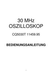
Fig. 4 shows the resonance curves of the current for different resistances. The strong influence of the resistance 

on the quality of the resonance is obvious. The 𝑄-factors calculated from the bandwidth are given 

in Tab.1. 

Tab. 1: Current resonance curves: bandwidths and quality 

factors for the series-tuned circuit. 

resistance bandwidth quality factor 

0 Ω 2 kHz 5.5 

47 Ω 8 kHz 1.4 

100 Ω 11 kHz 1.0 

4 PHYWE Systeme GmbH & Co. KG © All rights reserved P2440601 

(10)





As had been shown in the theory-section, the eigenfrequency of a tuned circuit depends on the inductance 

as well as the capacity in the circuit. Fig. 5 displays that dependence for the voltage resonance in 

the series-tuned circuit. 

Fig. 5: Terminal voltage as a function of frequency in the series tuned circuit. 

Task 2: Analyze the frequency performance of a parallel-tuned circuit. 

A loss resistance of 1460 Ω was found for the parallel-tuned circuit. The 𝑄-factors determined from Fig. 6 

are listed in Tab. 2. 

Tab.: 2 Voltage resonance curves: bandwidths and quality 

factors for the parallel-tuned circuit. 

resistance bandwidth quality factor 

470 Ω 8 kHz 1.4 

1000 Ω 6 kHz 1.8 

∞ 4 kHz 2.8 

Fig. 7 shows the current resonance in the parallel-tuned circuit for the second capacitor. 

For the resonance frequencies the found values of 11 kHz and 3.25 kHz with 𝐶 = 0.1 µF and 𝐶 = 1.0 µF 

respectively agree within 5 %. 

www.phywe.com 


TEP 




Fig. 6: Voltage as a function of frequency in the parallel-tuned circuit. 

Fig.: 7 Current as a function of frequency in the parallel-tuned circuit. 

6 PHYWE Systeme GmbH & Co. KG © All rights reserved P2440601

LEP 4.4.06 -01 RLC Circuit - Phywe Systeme GmbH

You also want an ePaper? Increase the reach of your titles

Delete template?

Save as template?