When Feedback Doubles the Prelog in AWGN Networks - Sites ...

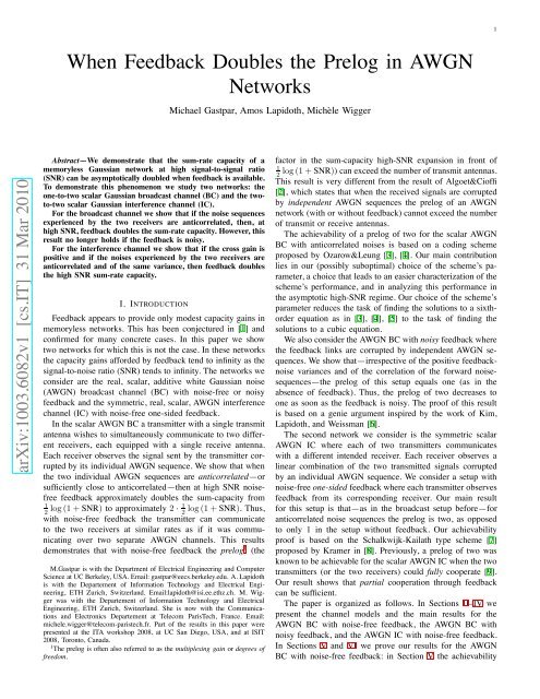
2M 1 ,M 2✲Fig. 1.D ✛❄Trans. X t✻D ✛✲✲Y✐❄ Z 1,t 1,t✲Y✐❄ Z 2,t 2,t✲Receiv.1Receiv.2The two-user AWGN BC with noise-free feedback.ˆM 1 ✲ˆM 2 ✲of prelog 2 for anticorrelated noises and a more generalachievability result for approximately anticorrelated noises;and in Section VI the rest of our results. In Section VII weprove our results for the AWGN BC with noisy feedback.In Sections VIII and IX we finally prove our results for theAWGN IC with noise-free one-sided feedback: in Section VIIIthe achievability of prelog 2 for anticorrelated noises; and inSection IX the rest of our results.II. BROADCAST CHANNEL WITH NOISE-FREE FEEDBACKA. The ModelThe real, scalar, AWGN BC with noise-free feedback isdepicted in Figure 1. Denoting the time-t transmitted symbolby x t ∈ R, thesymbolY 1,t that Receiver 1 receives at time-tisY 1,t = x t + Z 1,t , (1)and the symbol Y 2,t that Receiver 2 receives at time-t isY 2,t = x t + Z 2,t , (2)where the sequence of pairs {(Z 1,t ,Z 2,t )} is drawn independentlyand identically distributed (IID) according to a bivariatezero-mean Gaussian distribution of covariance matrix( )σ2K = 1 ρ z σ 1 σ 2ρ z σ 1 σ 2 σ22 . (3)We assume that σ1 2 and σ2 2 are positive and refer to them asthe noise variances and to ρ z ∈ [−1, 1] as the noise correlationcoefficient.The transmitter wishes to send Message M 1 to Receiver 1and an independent message M 2 to Receiver 2. The messagesM 1 and M 2 are assumed to be uniformly distributed overthe sets M 1 {1,...,⌊2 nR1 ⌋} and M 2 {1,...,⌊2 nR2 ⌋},where n denotes the blocklength and R 1 and R 2 the respectiverates of transmission.It is assumed that the transmitter has access to noise-freefeedback from both receivers, i.e., that after sending x t−1 itlearns both outputs Y 1,t−1 and Y 2,t−1 .Thetransmittercanthus compute its time-t channel input as a function of bothmessages and all previous channel outputs:X t = f (n) (BC,t M1 ,M 2 ,Y1 t−1 ,Y2t−1 ), t ∈{1,...,n}, (4)where the encoding function f (n)BC,tis of the formf (n)BC,t : M 1 ×M 2 × R t−1 × R t−1 → R (5)and where Y1 t−1 (Y 1,1 ,...,Y 1,t−1 ) and Y2 t−1 (Y 2,1 ,...,Y 2,t−1 ).The channel inputs are subject to an expected average blockpowerconstraint Pencoding functions[ n1n E ∑t=1({ > 0. Thus, in (4) we only allow fornfBC,t} (n) that satisfyt=1f (n)t(M 1 ,M 2 ,Y t−11 ,Y2 t−1 )) 2]≤ P. (6)After the n-th channel use each receiver decodes its intendedmessage based on its observed channel output sequence.Receiver 1 produces the guessand Receiver 2 the guessˆM 1 = φ (n)ˆM 2 = φ (n)1 (Y 1 n2 (Y 2 n), (7)), (8)where the decoding functions φ (n)1 and φ (n)2 are of the formφ (n)1 : R n →{1,...,⌊2 nR1 ⌋}, (9)φ (n)2 : R n →{1,...,⌊2 nR2 ⌋}. (10)A rate pair (R 1 ,R 2 ) is said to be achievable if forevery block-length { n there exists a set of n encodingnfunctions fBC,t} (n) as in (5) satisfying the power constraint(6) and two decoding functions φ (n)1 and φ (n)2 ast=1in [(9) and (10) such that the probability of decoding errorPr (M 1 ,M 2 ) ≠(ˆM 1 , ˆM]2 ) tends to 0 as the blocklength ntends to infinity, i.e.,[lim Pr (M 1 ,M 2 ) ≠(ˆM 1 , ˆM]2 ) =0.n→∞The closure of the set of all achievable rate pairs (R 1 ,R 2 ) iscalled the capacity region of this setup. The supremum of thesum R 1 + R 2 over all achievable rate pairs (R 1 ,R 2 ) is calledits sum-capacity, andwedenoteitbyC BC,Σ (P, σ 2 1 ,σ2 2 ,ρ z). Inthis paper we are particularly interested in the prelog, whichcharacterizes the logarithmic growth of the sum-capacity athigh powers, and is defined as:B. ResultsC BC,Σ (P, σlim1,σ 2 2,ρ 2 z )P →∞12 log(1 + P ) . (11)It is well known [10] that for the AWGN BC without feedbackthe prelog equals 1, irrespective of the noise-correlationρ z .ThefollowingTheorem1showsthatwithfeedbacktheprelog can be 2.Theorem 1:• If ρ z = −1, then• If ρ z ∈ (−1, 1), thenC BC,Σ (P, σ1 2 lim,σ2 2 ,ρ z)P →∞12 log(1 + P ) =2. (12)C BC,Σ (P, σ1 2 lim,σ2 2 ,ρ z)P →∞12 log(1 + P ) =1. (13)

4Fig. 4.M 1✲M 2✲D❄✛X 1,tTrans.1 ✲❅❘·a ✐ ✒·a ✐ ❅ ❅❘Trans.2 ✒ ✲✻X 2,tD ✛✐❄ Z 1,tY 1,t✲✐❄ Z 2,t✲Y 2,tReceiv.1Receiv.2The two-user AWGN IC with one-sided noise-free feedback.ˆM 1 ✲ˆM 2 ✲( )σdiagonal 2 2covariance matrix W 1 00 σW 2 .Weshallassume2throughout that the feedback noise variances are positiveσ W 1 ,σ W 2 > 0. (22)In this setup the transmitter computes its channel inputs asX t = f (n) (BCNoisy,t M1 ,M 2 ,V1 t−1 ,V2t−1 ), t ∈{1,...,n},(23)where the encoding function f (n)BCNoisy,tis of the formf (n)BCNoisy,t : M 1 ×M 2 × R t−1 × R t−1 → R, (24)and where V t−11 (V 1,1 ,...,V 1,t−1 ) and V t−12 (V 2,1 ,...,V 2,t−1 ).The channel input sequence is again subject to an expectedaverage block-power constraint P>0 as in (6).The decoding rules, achievable rates, capacity region, sumcapacityand prelog are defined as in the previous section. Thesum-capacity for this setup with noisy feedback is denoted byC BCNoisy,Σ (P, σ 2 1 ,σ2 2 ,ρ z,σ 2 W 1 ,σ2 W 2 ).B. ResultNoisy feedback does not increase the prelog.Theorem 4: Irrespective of the correlation ρ z ∈ [−1, 1], theprelog is one:C BCNoisy,Σ (P, σlim1,σ 2 2,ρ 2 z ,σW 2 1 ,σ2 W 2 )P →∞12 log (1 + P ) =1.Proof: See Section VII.IV. INTERFERENCE CHANNEL WITH NOISE-FREEFEEDBACKThe real scalar AWGN IC with noise-free feedback is depictedin Figure 4. Unlike the broadcast channel, this channelhas two transmitters, each of which wishes to send a messageto its corresponding receiver.A. The ModelTransmitter 1 wishes to send Message M 1 to Receiver 1, andTransmitter 2 wishes to send Message M 2 to Receiver 2. Themessages M 1 and M 2 are as defined previously. We assumea symmetric channel: ifattimet Transmitter 1 sends the real2 For simplicity, we do not treat setups with correlated feedback noises orsetups with feedback noises that are correlated with the forward noises.symbol x 1,t and Transmitter 2 sends the real symbol x 2,t ,thenReceiver 1 observesand Receiver 2 observesHere the “cross gain” aY 1,t = x 1,t + ax 2,t + Z 1,t , (25)Y 2,t = ax 1,t + x 2,t + Z 2,t . (26)a>0, (27)is a positive, real constant and the noise sequences{(Z 1,t ,Z 2,t )} are IID according to a zero-mean bivariateGaussian ( distribution ) of symmetric covariance matrix K =1σ 2 ρz.ρ z 1Each transmitter has access to noise-free feedback fromits corresponding receiver. Thus, each of the two transmitterscomputes its time-t channel input asX ν,t = f (n)IC,ν,t(Mν ,Y t−1ν), ν ∈{1, 2},for some encoding functions f (n)IC,ν,tof the formf (n)IC,ν,t : M ν × R t−1 → R, ν ∈{1, 2}.The two channel input sequences are subject to the sameaverage block-power constraint P>0:[ n1n E ∑ (f (n) (IC,ν,t Mν ,Yνt−1 ) ) ]2≤ P, ν ∈{1, 2}. (28)t=1Decoding rules, achievable rate pairs, capacity region, sumcapacity,and prelog are defined as for the AWGN BC. Wedenote the sum-capacity of the symmetric AWGN IC byC IC,Σ (P, σ 2 ,ρ z ,a).In this paper, we do not consider negative cross gains, becausethe (feedback) capacity region of the symmetric AWGNIC with cross gain a, powerconstraintsP ,noisevarianceσ 2 ,and noise correlation ρ z coincides with the (feedback) capacityregion of the symmetric AWGN IC with cross gain (−a),power constraints P ,noisevarianceσ 2 ,andnoisecorrelation(−ρ z ).Indeed,inasymmetricAWGNICwithparametersa, P, σ 2 ,ρ z Transmitter 2 and Receiver 2 (or Transmitter 1and Receiver 1) can simulate an AWGN IC with parameters(−a),P,σ 2 , (−ρ z ). This is accomplished if Transmitter 2multiplies its inputs {X 2,t } by −1 before feeding them to thechannel (which obviously does not affect the transmit power)and if Transmitter 2 and Receiver 2 multiply the outputs {Y 2,t }by −1 before processing them.B. ResultWithout feedback, the prelog of the AWGN IC equals 1;with noise-free feedback it can be 2, depending on the noisecorrelation ρ z ∈ [−1, 1].Theorem 5: The prelog of the AWGN IC with noise-freefeedback satisfies the following three statements.• If ρ z = −1, thentheprelogisgivenbyC IC,Σ (P, σ 2 ,ρ z ,a)limP →∞12 log(1 + P ) =2. (29)

5• If ρ z ∈ (−1, 1), thentheprelogisgivenbyC IC,Σ (P, σ 2 ,ρ z ,a)limP →∞12 log(1 + P ) =1. (30)• If ρ z =1,thentheprelogsatisfiesC IC,Σ (P, σ 2 ,ρ z ,a)1 ≤ limP →∞12 log(1 + P ) ≤ 2. (31)Moreover, when the cross gain a is equal to 1, theprelogis more precisely given byProof: See Section IX.C IC,Σ (P, σ 2 ,ρ z ,a)limP →∞12 log(1 + P ) =1. (32)V. ACHIEVABILITY OF PRELOG LARGER THAN 1 FOR THEAWGN BC WITH NOISE-FREE FEEDBACKIn this section we consider the AWGN BC with noisefreefeedback, and prove the achievability of prelog 2 whenρ z = −1 and the more general achievability result (19).These asymptotic results are achieved by the Ozarow-Leungscheme [3], [4] when the scheme’s parameter is chosen appropriately.For completeness, we briefly describe the Ozarow-Leung scheme with such an appropriate choice of parameter(Section V-A) and analyze its performance (Section V-B). Wefinally analyze the high-SNR asymptotics of the sum-ratesachieved by this scheme (Sections V-C and V-D).A. SchemeThe scheme by Ozarow and Leung [3], [4] (see also [5] and[8]) is based on the iterative strategy proposed by Schalkwijkand Kailath [7].Prior to transmission, the transmitter maps the Message M ν ,for ν ∈{1, 2}, intoaMessagepointΘ ν :Θ ν 1/2 − M ν − 1⌊2 nRν ⌋ . (33)It then describes Message point Θ ν in n channel uses toReceiver ν.The transmission starts with an initialization phase consistingof the first two channel uses. Channel use ν ∈{1, 2} isdedicated to Receiver ν only, and the transmitter sends√ (√)P PX ν =P + σN2 Var(Θ ν ) Θ ν + N ,where Var(Θ ν ) denotes the variance of the random variableΘ ν and where N is a zero-mean Gaussian random variableof variance σN 2 independent of the messages M 1 and M 2and of the noise sequence {(Z 1,t ,Z 2,t )}. 3 At the end of thisinitialization phase, each receiver estimates its desired message3 The described scheme can easily be turned into a deterministic scheme ofthe same asymptotic probability of error using a trick introduced in [11] andapplied in the scheme in Section VIII-A.point. Specifically, Receiver ν, forν ∈{1, 2}, producestheestimate ˆΘ ν,2 based on channel output Y ν,ν :√ √Var(Θν ) P + σ2ˆΘ ν,2 NY ν,νP√P√Var(Θν ) P + σ2=Θ ν +N(N + Z ν,ν ),P Pand thus has an estimation error:√ √ɛ ν,2 ˆΘ Var(Θν ) P + σ2ν,2 − Θ ν =N(N + Z ν,ν ).P PThe subsequent n − 2 channel uses are used to refine thereceivers’ estimates. To this end, the transmitter sends in eachsubsequent channel use t ∈{3,...,n} alinearcombinationof Receiver 1’s estimation error ɛ 1,t−1 about Message pointΘ 1 and of Receiver 2’s estimation error ɛ 2,t−2 about Messagepoint Θ 2 .Noticethatthetransmitterknowstheseestimationerrors because it is cognizant of both message points Θ 1 andΘ 2 ,andthroughthefeedback,alsoofthereceivers’estimates.Specifically, at time t ∈{3,...,n} the transmitter sendswhereandX t =ρ t−1 √P1+γ 2 +2γ|ρ t−1 |(ɛ1,t−1· √ + γsign(ρ t−1 ) ɛ )2,t−1√ ,α1,t−1 α2,t−1α ν,t−1 Var(ɛ ν,t−1 ) ,Cov[ɛ 1,t−1 ,ɛ 2,t−1 ]√Var(ɛ1,t−1 ) √ Var(2,t− 2) ,and where sign(·) denotes the signum function, i.e., sign(x) =1 if x ≥ 0 and sign(x) =−1 otherwise. The parameter γ is(possibly suboptimally) chosen asγ σ 1σ 2. (34)After each channel use t ∈{3,...,n} the two receivers updatetheir message-point estimates according to the rule:ˆΘ ν,t = ˆΘ ν,t−1 − Cov[ɛ ν,t−1,Y ν,t ]Y ν,t , ν ∈{1, 2}. (35)Var(Y ν,t )Each receiver decodes its intended message as follows. Afterthe reception of the n-th channel output, each Receiver νproduces as its guess the message ˆM ν whose message pointis closest to its last estimate ˆΘ ν,n ,i.e.,∣ˆM ν = argmin m∈{1,...,⌊e nRν ⌋} ∣Θ ν (m) − ˆΘ∣ ∣∣ν,n ,where ties can be resolved arbitrarily.

6B. Analysis of PerformanceWe only present a rough analysis of the scheme. For detailssee [3], [4].The probability of error of the described scheme tends to 0as the blocklength n tends to infinity, if:n∑1R ν < limn→∞ nhere α ν,1 Var(Θ ν ),α ν,2 Var(Θ ν)Pt=2( )12 log αν,t−1, ν ∈{1, 2}; (36)α ν,tP + σN2 (σN 2 + σ 2Pν), ν ∈{1, 2},and the variances {α 1,t } n t=3 and {α 2,t } n t=3 are defined throughthe recursions:σ 1σα 1,t = α 2P (1 − ρ 2 t−1 )+σ2 1 ( σ1σ 2+ σ21,t−1and( σ1σ 2σ 1+2|ρ t−1 |)+ σ2σ 1+2|ρ t−1 |)(P + σ1 2) , (37)σ 2σα 2,t = α 1P (1 − ρ 2 t−1 )+σ2 2 ( σ1σ 2+ σ22,t−1( σ1σ 2σ 1+2|ρ t−1 |)+ σ2σ 1+2|ρ t−1 |)(P + σ2 2) . (38)The sequence of correlation coefficients {ρ t } n t=2 is defined asρ 2 Cov[ɛ 1,2 ,ɛ 2,2 ]√Var(ɛ1,2 ) Var(ɛ 2,2 ) =σ 2 N√ √σ2N+ σ12 σ2N+ σ22(39)and for t ∈{3,...,n} through Recursion (40) on top of thenext page. We shall choose the variance σN2 such that thesequence {ρ t } n t=2 is constant in magnitude but alternates insign, i.e., such that for some ρ ∗ ∈ (0, 1):ρ t =(−1) t ρ ∗ , t ∈{2,...,n}. (41)This way, the ratios α1,t−1α 1,tand α2,t−1α 2,tare constant for t ∈{3,...,n}, andtriviallythelimitontheright-handsideof(36) equalsn∑( )12 log αν,t−1αt=2ν,t⎛= 1 2 log ⎝2P + σν21limn→∞ nσ 2 νσ 2 1 +σ2 2 +2σ1σ2ρ∗ P (1 − (ρ ∗ ) 2 )+σ 2 ν⎞⎠ . (42)By Equation (39), we can set the correlation coefficient ρ 2to every desired value in [0, 1) if we choose the varianceσN2 appropriately. Therefore, Condition (41) can be satisfiedfor all ρ ∗ ∈ [0, 1) with the following “fixed point” property:substituting ρ ∗ for ρ t−1 in Recursion (40) yields ρ t = −ρ ∗ ,and similarly, substituting −ρ ∗ for ρ t−1 in Recursion (40)yields ρ t = ρ ∗ .In[3],[4]itwasshownthatRecursion(40)hasat least one such “fixed point”. Also, using simple algebraicmanipulations, the “fixed points” ρ ∗ of Recursion (40) arefound to be the solutions in (0, 1) to the following cubicequation in ρ:wherec 2 − 2σ 1σ 2Pρ 3 + c 2 ρ 2 + c 1 ρ + c 0 =0, (43)− P + σ2 1 + σ2 2 + ρ zσ 1 σ 2√ √P + σ21 P + σ222σ 2 1 σ2 2−P √ √ , (44)P + σ12 P + σ22(σ1 2 + σ− ρ2)2z √ √P + σ21 P + σ22c 1 −1 − σ2 1 + σ 2 2P− σ 1σ 2 (σ1 2 + σ2 2 )P √ √ , (45)P + σ12 P + σ22c 0 P + σ2 1 + σ2 2 − ρ z σ 1 σ√ √ 2. (46)P + σ21 P + σ22Combining these observations with (36) and (42), we obtainthe following lemma.Lemma 1: Choosing the parameter γ as in (34), theOzarow-Leung scheme achieves all nonnegative rate pairs(R 1 ,R 2 ) satisfying⎛⎞R 1 < 1 2 log ⎝P + σ12 ⎠2, (47)σ12 P (1 − (ρσ ∗ ) 2 )+σ 21 2+σ2 2 +2σ1σ2ρ∗ 1⎛⎞R 2 < 1 2 log ⎝P + σ22 ⎠2, (48)σ22 P (1 − (ρσ ∗ ) 2 )+σ 21 2+σ2 2 +2σ1σ2ρ∗ 2where ρ ∗ is a 4 solution in the open interval (0, 1) to the cubicequation (43).Remark 1: To characterize the scheme’s performance for ageneral parameter γ requires finding the solutions to a sixthorderequation [3], [4]. Our (possibly suboptimal) choice ofγ in (34) makes it possible to find the scheme’s performancewhile solving only a cubic equation; see (43).C. High-SNR asymptotics for constant ρ z = −1In this section we prove that the above described schemeachieves prelog 2 when ρ z = −1.Proposition 6: When ρ z = −1 the Ozarow-Leung schemewith parameter γ = σ1σ 2achieves prelog 2.Proof: Let ρ z be −1. ByLemma1,foreverypowerPand every ɛ>0 the Ozarow-Leung scheme with parameterγ = σ1σ 2achieves a sum-rateR Σ (P )⎛= 1 2 log ⎝+ 1 2 log ⎛⎝P + σ12σ1 2(1+ρ∗ (P ))σ1 2+σ2 2 +2σ1σ2ρ∗ (P ) P (1 − ρ∗ (P )) + σ12⎞⎠P + σ22σ2 2(1+ρ∗ (P ))σ1 2+σ2 2 +2σ1σ2ρ∗ (P ) P (1 − ρ∗ (P )) + σ22⎞⎠ − ɛ,where the parameter ρ ∗ (P ) is defined as a solution in (0, 1)to the cubic equation (43).Since for each power P > 0 the parameter ρ ∗ (P ) lies inthe open interval (0, 1), wehaveσ1 2(1 + ρ∗ (P ))σ1 2 + σ2 2 +2σ 1σ 2 ρ ∗ (P ) ≤ 2σ2 1σ1 2 + , σ2 2(49)σ2 2(1 + ρ∗ (P ))σ1 2 + σ2 2 +2σ 1σ 2 ρ ∗ (P ) ≤ 2σ2 2σ1 2 + , σ2 2(50)4 If there is more than one solution in [0, 1] to (43) we can freely chooseone. Numerical results suggest that there is only one solution.

7√ √P + σ2ρ t = sign(ρ t−1 ) ·1 P + σ22P (1 −|ρ t−1 | 2 )+(σ1 2 + σ2 2 +2σ 1σ 2 |ρ t−1 |)( (σ1· |ρ t−1 | + σ ) ( )( )2σ1σ2 P (P + σ2+2|ρ t−1 | − + |ρ t−1 | + |ρ t−1 |1 + σ 2 )2 − ρ z σ 1 σ 2 )σ 2 σ 1 σ 2 σ 1 (P + σ1 2)(P + σ2 2 )(40)and we can thus lower bound the achievable sum-rate R Σ (P )by⎛⎞R Σ (P ) ≥ 1 2 log ⎝P + σ12 ⎠2σ12 P (1 − ρσ ∗ (P )) + σ 21 2+σ2 12⎛⎞+ 1 2 log ⎝P + σ22 ⎠ − ɛ. (51)2σ22 P (1 − ρσ ∗ (P )) + σ 21 2+σ2 22The desired lower bound on the preloglimP →∞R Σ (P )1≥ 2,2log (1 + P )is then obtained from (51) by showing that as P →∞the sequenceof solutions {ρ ∗ (P )} {P>0} tends to -1 approximatelyas −1+P −1 .ThisfollowsfromLemma2thatwestatenext.Lemma 2: Let ρ z be −1. ForeachpowerP>0 let ρ ∗ (P )be the solution in the interval (0, 1) to (43). Then, for everyɛ>0lim P 1−ɛ (1 − ρ ∗ (P )) = 0. (52)P →∞Proof: The result could be proved by first computing foreach P>0 the solution ρ ∗ (P ) to the cubic equation (43) (e.g.,using Cardano’s formula), and then analyzing the asymptoticsof the solutions as P → ∞. However, this line of attackis rather cumbersome. Instead, we show that if a sequence{ρ ∗ (P )} {P>0} in (0, 1) violates (52) for some ɛ>0, thenthere exists some power P>0 such that ρ ∗ (P ) cannot be asolution to (43). For details, see Appendix A.D. High-SNR asymptotics for ρ z (P ) varying with PWe prove the more general asymptotic high-SNR achievabilityresult in (19).Proposition 7: Fix a sequence {ρ z (P )} {P>0} and definethe limit β as in (17):β = limP →∞− log(1 + ρ z (P )).log(P )The Ozarow-Leung scheme with parameter γ = σ1σ 2achievessum-rates {R Σ (P )} {P>0} satisfyingR Σ (P )limP →∞1≥ min{1+β,2}. (53)2log(1 + P )Proof: By Lemma 1 and Inequalities (49) and (50) inthe previous subsection, for each power P > 0 and ɛ>0,the Ozarow-Leung scheme with parameter γ = σ1σ 2achieves asum-rate R Σ (P ) that is lower bounded by⎛⎞R Σ (P ) ≥ 1 2 log ⎝P + σ12 ⎠2 2σ12 P (1 − ρσ ∗ (P )) + σ 21 2+σ2 12⎛⎞+ 1 2 log ⎝P + σ22 ⎠2− ɛ, (54)2σ22 P (1 − ρσ ∗ (P )) + σ 21 2+σ2 22where ρ ∗ (P ) is defined as a solution in (0, 1) to the cubicequation (43). The desired asymptotic lower bound (53) thenfollows from (54) and the following Lemma 3.Lemma 3: for each power P > 0, letanoisecorrelationρ z (P ) ∈ [−1, 1] be given, and let ρ ∗ (P ) be a solution in(0, 1) to the cubic equation in (43). Then,lim P 1−ɛ (1 − ρ ∗ (P )) = 0,P →∞Proof: See Appendix B.{ 1 − β∀ɛ >max2}, 0 .VI. PROOFS OF THEOREMS 1 AND 2 AND NOTE 1 FOR THEAWGN BC WITH NOISE-FREE FEEDBACKAs mentioned in Note 2, Relations (12)–(14) in Theorem 1can be directly obtained from Theorem 2. Nevertheless, forconvenience to the reader we provide a separate proof for eachof the relations in Theorem 1.A. Proof of Theorem 1Equation (14) follows from the following more generalrelation: irrespective of the noise correlation ρ z ∈ [−1, 1] andthe noise variances σ 2 1,σ 2 2 > 0 the prelog satisfiesC BC,Σ (P, σ1 ≤ lim1,σ 2 2,ρ 2 z )P →∞12 log(1 + P ) ≤ 2. (55)The lower bound in (55) holds because without feedback theprelog of the AWGN BC equals 1 irrespective of ρ z ∈ [−1, 1](see the capacity result of the AWGN BC without feedback in[10]). The upper bound in (55) holds because whenever a ratepair (R 1 ,R 2 ) is achievable over the AWGN BC with noisefreefeedback, then the rates R 1 and R 2 cannot exceed thesingle-user capacities (with feedback) of the AWGN channelsfrom the transmitter to the corresponding receiver, i.e.,R ν ≤ 1 2 log (1+ P σ 2 ν), ν ∈{1, 2}. (56)Equation (12) follows from Relation (55) and Proposition 6.We next establish Equation (15). Notice that when ρ z =1and σ 2 1 = σ 2 2,thetwonoisesequences{Z 1,t } and {Z 2,t }coincide, and thus the two receivers observe exactly the sameoutput sequences, i.e., Y 1,t = Y 2,t at all time instances t ∈{1,...,n}. Consequently,ifReceiver2candecodeM 2 ,thenso can Receiver 1 and hence (R 1 ,R 2 ) can be achievable onlyif R 1 + R 2 does not exceed the capacity of the channel toReceiver 1. This implies that the sum-capacity of the AWGNBC with noise-free feedback coincides with the single-user

8feedback capacity of the AWGN channel from the transmitterto one of the two receivers:C BC,Σ (P, σ 2 ,σ 2 ,ρ z =1)= 1 (2 log 1+ P )σ 2 . (57)This establishes the desired result in (15).We finally prove Equation (13). By Relation (55) it sufficesto show that when ρ z lies in the open interval (−1, 1), thenthe prelog is upper bounded by 1. Invoking the cutset bound[12, Theorem 15.10.1] with a cut between the transmitter andboth receivers we can upper bound the sum-capacity asC BC,Σ (P, σ 2 1,σ 2 2,ρ z ) ≤ max I(X; Y 1 Y 2 ), (58)where the maximization is over all input distributions on Xsatisfying E [ X 2] ≤ P .Bytheentropymaximizingpropertyof the Gaussian distribution under a covariance matrix constraint[12], the upper bound in (58) is equivalent to⎛⎞PC BC,Σ (P, σ1 2 ,σ2 2 ,ρ z) ≤ 1 ⎝1+2σ 2 1 σ2 2σ 2 1 +σ2 2⎠ , (59)(1 − ρ 2 z)which establishes that for every ρ z ∈ (−1, 1) the prelog isupper bounded by 1.B. Proof of Theorem 2The asymptotic upper bound (18) follows again from thecutset bound and the entropy maximizing property of Gaussiandistributions under a covariance constraint. In fact, applyingthe cutset bound with a cut between the transmitter and bothreceivers (in analogy to (59)) for given power P > 0, noisevariances σ 2 1 ,σ2 2 > 0, andnoisecorrelationρ z(P ) ∈ (−1, 1)we can upper bound the sum-capacity asC BC,Σ (P, σ1 2 ,σ2 2 ,ρ z(P ))⎛≤ 1 2 log ⎝1+≤ 1 2 log ⎛⎝1+σ 2 1 σ2 2σ 2 1 +σ2 22 σ2 1 σ2 2σ 2 1 +σ2 2⎞P⎠(1 −|ρ z (P )| 2 )⎞P⎠ , (60)(1 −|ρ z (P )|)where in the second inequality we used that ρ z (P ) ∈ (−1, 1).Moreover—as argued in (56)—the sum-capacity cannot exceedthe sum of the two single-user capacities of the channelsfrom the transmitter to the two receivers, i.e.,C BC,Σ (P, σ1,σ 2 2,ρ 2 z )≤ 1 (2 log 1+ P )σ12 + 1 (2 log 1+ P )σ22 . (61)The asymptotic upper bound (18) follows then by combining(60) and (61) with the definition of α in (16).The asymptotic lower bound (19) follows from Proposition7 in Section V-D.C. Proof of Note 1We have to show that the achievability results in Theorem 1remain valid also in the weaker setup with only one-sidedfeedback. The achievability results in (13) and (14) remainvalid because a prelog of 1 is trivially achievable for all valuesof ρ z ∈ [−1, 1] even without feedback [10]. The achievabilityresult in (12) remains valid because for ρ z = −1 the capacityregions of the setups with one-sided and two-sided feedbackcoincide. In fact, after each channel use t the transmitter canlocally compute the missing output Y 2,t (or Y 1,t )fromtheobserved feedback output Y 1,t (or Y 2,t )andtheinputX t :Y 2,t = − σ 2σ 1(Y 1,t − X t )+X t ,t ∈{1,...,n}.VII. PROOF OF THEOREM 4 FOR THE AWGN BC WITHNOISY FEEDBACKSince for all correlation coefficients ρ z ∈ [−1, 1] prelog 1is achievable even without feedback [10], the interesting partof Theorem 4 is the converse result. We prove this converseresult using a genie-argument similar to [6].Our proof is based on the following three steps. In thefirst step we introduce a genie-aided AWGN BC withoutfeedback and show that its sum-capacity upper bounds thesum-capacity of the original AWGN BC with noisy feedback.In the second step we introduce a less noisy AWGN BC withneither genie-information nor feedback and show that its sumcapacitycoincides with the sum-capacity of the genie-aidedAWGN BC. In the third step, we finally show that the prelogof the less noisy AWGN BC equals 1, irrespective of the noisevariances σ1,σ 2 2,σ 2 W 2 1 ,σ2 W 2 > 0 and the correlation coefficientρ z ∈ [−1, 1]. Thesethreestepsestablishthedesiredconverseresult.We elaborate on these three steps starting with the firstone. The genie-aided AWGN BC is defined as the originalAWGN BC without feedback, butwithageniethatpriortotransmission reveals the sequences {(Z 1,t + W 1,t )} n t=1 and{(Z 2,t +W 2,t )} n t=1 to the transmitter and both receivers. Noticethat with this genie information, after each channel use t, thetransmitter can locally compute the missing feedback outputsV 1,t and V 2,t :V 1,t = X t +(Z 1,t + W 1,t ), (62)V 2,t = X t +(Z 2,t + W 2,t ). (63)We can thus conclude that the sum-capacity of the genie-aidedAWGN BC is at least as large as the sum-capacity of theoriginal AWGN BC with feedback.We next elaborate on the second step. The less noisy AWGNBC is described by the channel law:where the noise sequences are defined asỸ 1,t = x t + ˜Z 1,t , (64)Ỹ 2,t = x t + ˜Z 2,t , (65)˜Z 1,t Z 1,t − E[Z 1,t |(Z 1,t + W 1,t ), (Z 2,t + W 2,t )] , (66)˜Z 2,t Z 2,t − E[Z 2,t |(Z 1,t + W 1,t ), (Z 2,t + W 2,t )] , (67)

9and are of variances( )Var ˜Z1,t = σ12 σW 2 1 σ2 2(1 − ρ 2 z)+σW 2 1 σ2 W 2(σ1 2 + σ2 W 1 )(σ2 2 + σ2 W 2 ) − , (68)σ2 1 σ2 2 ρ2 z( )Var ˜Z2,t = σ22 σW 2 2 σ2 1(1 − ρ 2 z)+σW 2 2 σ2 W 1(σ1 2 + σ2 W 1 )(σ2 2 + σ2 W 2 ) − . (69)σ2 1 σ2 2 ρ2 zBy the following two observations, the sum-capacity of thisless noisy AWGN BC coincides with the sum-capacity of thegenie-aided AWGN BC. Firstly, the sum-capacity of the lessnoisy AWGN BC remains unchanged if prior to transmissionagenierevealsthesequences{Z 1,t +W 1,t } and {Z 2,t +W 2,t }to the transmitter and both receivers. This follows because byDefinitions (66) and (67) the genie-information {Z 1,t + W 1,t }and {Z 2,t + W 2,t } is independent of the reduced noise sequences{ ˜Z 1,t , ˜Z 2,t },andthusplaysonlytheroleofcommonrandomness which does not increase capacity. Secondly, thesum-capacity of the genie-aided AWGN BC coincides withthe sum-capacity of the less noisy AWGN BC, when in thislatter case the transmitter and both receivers additionallyknowthe genie-information {(Z 1,t + W 1,t )} and {(Z 2,t + W 2,t )}.This holds because knowing the genie-information {(Z 1,t +W 1,t )} n t=1 and {(Z 2,t + W 2,t )} n t=1 the outputs Ỹ1,t and Ỹ2,tcan be transformed into the outputs Y 1,t and Y 2,t ,andviceversa.We finally elaborate on the third step. The less noisy AWGNBC is a classical AWGN BC with neither feedback nor genieinformation,and its sum-capacity is given by [10]:C BCLessNoisy,Σ (P, σ1 2 ,σ2 2 ,ρ z,σW 2 1 ,σ2 W 2⎛) ⎞= 1 2 log P⎝1+ { ( ) ( )} ⎠ , (70)min Var ˜Z1,t , Var ˜Z2,t( ) ( )where the variances Var ˜Z1,t , Var ˜Z2,t are defined in(68) and (69). By (68)–(70) the prelog of the less noisyAWGN BC equals 1, irrespective of the noise variancesσ1 2,σ2 2 ,σ2 W 1 ,σ2 W 2 > 0 and the noise correlation ρ z ∈ [−1, 1].This concludes the third step, and thus our proof.VIII. ACHIEVABILITY OF PRELOG 2 FOR THE AWGN ICWITH NOISE-FREE FEEDBACKWe prove that the prelog of the AWGN IC with one-sidednoise-free feedback equals 2 when ρ z = −1. As in theprevious section, this prelog is achieved with a Schalkwijk-Kailath-type scheme. More specifically, it is achieved by astraightforward extension of Kramer’s memoryless-LMMSEscheme for interference channels [8, Section VI-B] to channelswith correlated noises.A. Scheme for ρ z = −1Prior to transmission, each transmitter maps its message intoamessagepointasin(33).Thetransmittersthendescribethesemessage points to their intended receivers using n channeluses.The first three channel uses are part of an initializationprocedure. In the first channel use both transmitters remainsilent. Via the feedback both transmitters then observe theGaussian random variable N Z 1,1 = −Z 2,1 ,whichwillserve them as common randomness in future transmissions.In the second channel use Transmitter 2 remains again silentand Transmitter 1 sends:√ (√)P PX 1,2 =P + σN2 Var(Θ 1 ) Θ 1 + N σ N,σwhere σ N will be defined later on. In the third channel useTransmitter 1 remains silent and Transmitter 2 sends:√ (√)P PX 2,3 =P + σN2 Var(Θ 2 ) Θ 2 + N σ N.σAt the end of this initialization √ phase Receiver 1 producesthe estimate ˆΘ√P +σN1,3 2 Var(Θ 1)P PY 1,2 and Receiver 2√the estimate ˆΘ√P +σN2,3 2 Var(Θ 2)P PY 2,3 .Theirestimationerrors are thus given by:√ √ɛ 1,3 ˆΘ Var(Θ1 ) P + σ21,3 − Θ 1 =N(N + Z 1,2 ),P Pandɛ 2,3 ˆΘ 2,3 − Θ 2 =√Var(Θ2 )P√P + σ2NP(N + Z 2,2 ).In the subsequent (n−3) channel uses, the two transmitterstransmit symbols in order to help the receivers refine theseestimates. In channel use t ∈{4,...,n}, Transmitter1sendsascaledversionofReceiver1’sestimationerrorɛ 1,t−1 aboutmessage point Θ 1 and Transmitter 2 sends Receiver 2’s estimationerror ɛ 2,t−2 about message point Θ 2 .Noticethateachtransmitter knows the estimation error of its correspondingreceiver because it is cognizant of its own message pointand through the noise-free one-sided feedback also of theestimate at its corresponding receiver. Specifically, at timet ∈{4,...,n} Transmitter 1 sendsX 1,t =√Pɛ 1,t−1 ,α 1,t−1and Transmitter 2 sendsX 2,t =√sign(ρ t−1 )Pɛ 2,t−1 .α 2,t−1After each channel use t ∈{4,...,n} the two receivers updatetheir message-point estimates according to the updating rule(35) in Section V-A.After the reception of the n-th channel output, Receiver νproduces as its guess the message ˆM ν whose message pointis closest to its estimate ˆΘ ν,n ,i.e.,∣ˆM ν = argmin m∈{1,...,⌊e nRν ⌋} ∣Θ ν (m) − ˆΘ∣ ∣∣ν,n ,where ties can be resolved arbitrarily.

10B. AnalysisWe present only a rough analysis of the scheme. For moredetails, see [8].The probability of error of the described scheme tends to 0as the blocklength n tends to infinity, if for ν ∈{1, 2}:1R ν ≤ limn→∞ nwhere α ν,2 = Var(Θ ν );α ν,3 = Var(Θ) νPand for t ∈{4,...,n}:n∑t=3P + σ 2 NP( )12 log αν,t−1, (71)α ν,t(σ 2 N + σ 2 ), ν ∈{1, 2}; (72)Pa 2 (1 −|ρ t−1 | 2 )+σ 2α ν,t = α ν,t−1P (1 + a 2 , ν ∈{1, 2}.+2a|ρ t−1 |)+σ2 (73)The correlation coefficients {ρ t } n t=3 are defined asρ 3 =σ 2 Nσ2 N+ σ2, (74)and for t ∈{4,...,n} through Recursion (75) on top of thenext page. We shall choose the variance σN2 such that thesequence {ρ t } n t=2 is constant in magnitude but alternates insign, i.e., such that for some ρ ∗ IC ∈ (0, 1):ρ t =(−1) t ρ ∗ IC , t ∈{3,...,n}. (76)This way, the ratios α1,t−1α 1,tand α2,t−1α 2,tare constant for t ∈{4,...,n}, andtriviallythelimitontheright-handsideof(71) equals1limn→∞ nn∑t=3( )12 log αν,t−1α ν,t= 1 ( P (1 + a 22 log +2aρ ∗ )IC )+σ2Pa 2 (1 − (ρ ∗ IC )2 )+σ 2 . (77)By Equation (74), we can set ρ 3 to every value in [0, 1) ifwe appropriately choose the variance σN 2 .Therefore,Condition(76) can be satisfied for all ρ ∗ ∈ [0, 1) that correspondto “fixed points” of Recursion (75), i.e., for all ρ ∗ such thatsubstituting ρ t−1 = ρ ∗ into Recursion (75) yields ρ t = −ρ ∗ ,and substituting ρ t−1 = −ρ ∗ into Recursion (75) yieldsρ t = ρ ∗ . Using simple algebraic manipulations it can beseen that the set of such “fixed points” is given by the setof solutions in [0, 1) to the quartic equationwhereρ 4 + d 3 ρ 3 + d 2 ρ 2 + d 1 ρ + d 0 =0, (78)d 3 =σ22aP , (79)d 2 = −2 − σ2 (4 + aρ z )2a 2 , (80)Pd 1 = − σ2 (1 + 2a 2 +2aρ z )2a 3 P−σ4a 3 P 2 , (81)d 0 =1+ σ2 (2a − ρ z )2a 3 . (82)PNotice that Equation (78) has at least one solution in [0, 1),and thus, Recursion (75) has at least one “fixed point” ρ ∗ IC in[0, 1). ThisfollowsbytheIntermediate-ValueTheoremandbecause for ρ =0and ρ z = −1 the left hand-side of (78)evaluates to 1+ σ2 (2a+1)2a 3 P> 0 and for ρ =1and ρ z = −1 itevaluates to − σ4a 3 P< 0. Combiningtheseobservationswith2(71) and (77) leads to the following lemma.Lemma 4: Let power P>0, noisevarianceσ 2 > 0, noisecorrelation ρ z ∈ [−1, 1], andcrossgaina ≠0be given. Thescheme described in Section VIII-A achieves all rate pairs(R 1 ,R 2 ) satisfyingR ν < 1 ( P (1 + a 22 log +2aρ ∗ )IC )+σ2Pa 2 (1 − (ρ ∗ IC )2 )+σ 2 , ν ∈{1, 2},(83)where ρ ∗ IC is defined as a solution5 in (0, 1) to the quarticequation (78).C. High-SNR AsymptoticsProposition 8: When ρ z = −1 and a > 0 the abovedescribed scheme achieves prelog 2.Proof: By Lemma 4, for each power P>0 and ɛ>0the scheme in the previous section VIII-A achieves a sum-rate( P (1 + a 2 ρ ∗ )ICR Σ (P ) = log)+σ2Pa 2 (1 − (ρ ∗ IC )2 )+σ 2 − ɛ( P (1 + a 2 )+σ 2 )≥ log2Pa 2 (1 − ρ ∗ − ɛ, (84)IC )+σ2where ρ ∗ IC is defined as a solution in (0, 1) to the quarticequation (78), and where the inequality follows because ρ ∗ IClies in the interval (0, 1).The desired asymptotic lower bound (29) follows from (84)and from the following Lemma 5.Lemma 5: Let the noise variance σ 2 > 0, noisecorrelationρ z = −1, andcrossgaina>0 be given. For each powerP>0 let ρ ∗ IC (P ) to be a solution in the interval (0, 1) to thequartic equation (78) in ρ. Then,lim P 1−ɛ (1 − ρ ∗ IC (P )) = 0, ∀ɛ >0.P →∞Proof: See Appendix C.IX. PROOF OF THEOREM 5 FOR THE AWGN IC WITHNOISE-FREE FEEDBACKWe first prove Relation (31), which follows from the followingmore general relation. Irrespective of the symmetricnoise-variance σ 2 > 0, thenoisecorrelationρ z ∈ [−1, 1], andthe cross gain a>0, theprelogsatisfiesC IC,Σ (P, σ, ρ z ,a)1 ≤ limP →∞12 log(1 + P ) ≤ 2. (85)The lower bound can be achieved, e.g., by silencing Transmitter1 and letting Transmitter 2 communicate its Message M 2 toReceiver 2 over the resulting interference-free AWGN channelY 2,t = X 2,t + Z 2,t at a rate R 2 = 1 2 log ( )1+ P σ .Theupper25 If there is more than one such solution, then one can freely choose oneof them.

11ρ t = sign(ρ t−1 ) P (1 + a2 +2a|ρ t−1 |)+σ 2Pa 2 (1 −|ρ 2 t−1(|)+σ2· |ρ t−1 − 2 P (a + |ρ t−1|)(1 + a|ρ t−1 |)P (1 + a 2 +2a|ρ t−1 |)+σ 2 + P (1 + a|ρ t−1 |) 2)(P (1 + a 2 +2a|ρ t−1 |)+σ 2 ) 2 (P (2a + |ρ t−1|(1 + a 2 )) + σ 2 ρ z ) .(75)bound can be derived using the cutset bound and the entropymaximizing property of the Gaussian distribution under acovariance matrix constraint. In fact, applying the cutset boundwith a cut between both transmitters and Receiver 2 on oneside and Receiver 1 on the other side yieldsR 1 ≤ max I(X 1 X 2 ; Y 1 )= 1 (2 log 1+ (1 + )a)2 Pσ 2 ,where the maximization is over all joint laws on the pair(X 1 ,X 2 ) satisfying the power constraints E [ X 2 1]≤ P andE [ X 2 2]≤ P .Similarly,applyingthecutsetboundwithacutbetween both transmitters and Receiver 1 on one side andReceiver 2 on the other side yieldsR 2 ≤ max I(X 1 X 2 ; Y 2 )= 1 (2 log 1+ (1 + )a)2 Pσ 2 .These two upper bounds establish the converse result in (31).Equation (29) is established by the general Relation (85)and Proposition 8 in Section VIII-C.We next establish Equation (32). Towards this end, wenotice that for a =1and ρ z =1the two output sequences{Y 1,t } and {Y 2,t } coincide. Therefore, whenever Receiver 1can decode its message M 1 so can Receiver 2, and similarlywhenever Receiver 2 can decode M 2 so can Receiver 1. Thus,for a =1and ρ z =1the feedback capacity of our AWGNIC coincides with the feedback capacity of the AWGN MACsfrom both transmitters to one of the two receivers. Since theseAWGN MACs have prelog 1 (with or without feedback) [13],[14], [15] Relation (32) follows.We finally show that irrespective of the cross gain a>0,for ρ z ∈ (−1, 1) the prelog is upper bounded by 1, i.e.,C IC,Σ (P, σ, ρ z ,a)limP →∞12 log(1 + P ) ≤ 1, ρ z ∈ (−1, 1). (86)Combined with (85) this establishes (30).We prove (86) based on a genie-argument and a generalizedSato-MAC bound [16], similar to the upper bounds in [17],[18]. Our proof consists of the following three steps. In thefirst step, we consider a scenario where prior to transmission agenie reveals the symbols U n = Z1 n − 1 a Zn 2 to Receiver 1. Thisobviously can only increase the sum-capacity of our channel.In the second step, we apply Sato’s MAC-bound argument[16] to the genie-aided AWGN IC obtained in the first step: 6 we6 Unlike in Sato’s setup, here both transmitters have feedback. As we shallsee, Sato’s MAC-bound argument applies unchanged also to feedback-setups,as the argument affects only the receivers.show that the capacity of this IC is included in the capacity ofthe MAC that results from the IC when Receiver 1 is requiredto decode both messages and Receiver 2 no message at all. Theinclusion can be proved based on the following observation.Whenever Receiver 1 has successfully decoded Message M 1 ,then it can reconstruct the inputs X1n and also the outputsobserved at Receiver 2:Y n2 = 1 a (Y n1 − X n 1 )+U n . (87)Consequently, under this assumption it can decode MessageM 2 in the same way as Receiver 2. This implies that forfixed encoding strategies applied at the two transmitters, theminimum probability of error in the MAC setup cannot exceedthe minimum probability of error in the IC setup and provesthe desired inclusion.In the third step we show that the MAC to Receiver 1 hasprelog no larger than 1. Combined with the previous two stepsthis yields the desired upper bound (86). Before elaboratingon this third step, we recall some properties of the consideredMAC: Its channel law is described byY 1,t = X 1,t + aX 2,t + Z 1,t ,t ∈{1,...,n};its two transmitters observe the generalized feedback signals{Y 1,t } and {Y 2,t }; and before the transmission starts itsreceiver learns the genie-information U n .We now prove that the prelog of this MAC is upper boundedby 1. To this end we fix an arbitrary sequence of blocklengthn,rates-(R 1 ,R 2 ) coding schemes for the considered MACsuch that the probability of error ɛ(n) tends to zero as n tendsto infinity. Then, for every blocklength n we have:R 1 + R 2≤1 n I(M 1,M 2 ; Y1 n ,U n )+ ɛ(n)n= 1 n I(M 1,M 2 ; Y1 n |U n )+ ɛ(n)n= 1 n∑ (h(Y 1,t |Y1 t−1 ,U n )nt=1)−h(Y 1,t |Y1 t−1 ,M 1 ,M 2 ,U n )≤1 n∑ (h(Y 1,t |U t )nt=1)−h(Y 1,t |Y1 t−1 ,M 1 ,M 2 ,Y2 t−1 ,U n )= 1 n∑ ()h(Y 1,t |U t ) − h(Y 1,t |X 1,t ,X 2,t ,U t )nt=1+ ɛ(n)n+ ɛ(n)n

12= 1 nn∑I(Y 1,t ; X 1,t ,X 2,t |U t )t=1≤ 1 2 log (1+ (1 + a)2 P)σ 2 1−ρ 2 z1+a 2 −2aρ z+ ɛ(n)n ,where the first inequality follows by Fano’s inequality; the firstequality follows by the independence of the genie-informationU n and the messages M 1 and M 2 ;thesecondinequalityfollowsbecause conditioning cannot increase differential entropyand because the vector Y2 t−1 can be computed as a functionof M 1 ,Y1 t−1 ,andU t−1 ,see(87);thethirdequalityfollowsbecause the input X 1,t is a function of the Message M 1 andthe feedback outputs Y1 t−1 ,andsimilarlyX 2,t is a functionof M 2 and Y2 t−1 ,andbecauseoftheMarkovrelation(M 1 ,M 2 ,Y t−11 ,Y t−12 ,U t−1 ,U n t+1 ) − (X 1,t,X 2,t ,U t ) − Y 1,t ;and the last inequality follows because the Gaussian distributionmaximizes differential entropy under a covarianceconstraint. Since by assumption the probabilities of error ɛ(n)tend to 0 as n →∞the sum-rate of the considered schememust satisfy()R 1 + R 2 ≤ 1 2 log 1+ (1 + a)2 P,σ 2 (1−ρ 2 z )1+a 2 −2aρ zand thus the sum-capacity of the MAC to Receiver 1()C MAC,Σ (P, σ 2 ,ρ z ,a) ≤ 1 2 log 1+ (1 + a)2 P.σ 2 (1−ρ 2 z )1+a 2 −2aρ zIt immediately follows that for a>0 and ρ z ∈ (−1, 1) theprelog is upper bounded by 1, which concludes the third stepand the proof of (86).ACKNOWLEDGMENTThe authors thank Prof. Frans M. J. Willems, TU Eindhoven,for pointing them to [5], which inspired the investigationleading to this work. This work was supported in part byNSF grants CNS-0627024 and CCF-0830428.A. Proof of Lemma 2APPENDIXSince for every P > 0 the parameter ρ ∗ (P ) lies in theinterval (0, 1):lim P 1−ɛ (1 − ρ ∗ (P )) ≥ 0, ∀ɛ >0.P →∞Thus, we have to prove thatlim P 1−ɛ (1 − ρ ∗ (P )) ≤ 0, ∀ɛ >0. (88)P →∞To this end, we introduce for every P>0 the parameterwhich by (43) and (44)–(46) satisfiesg ∗ (P ) 1 − ρ ∗ (P ), (89)0=− (g ∗ (P )) 3 + γ 2 (P )(g ∗ (P )) 2 + γ 1 (P )g ∗ (P )+γ 0 (P ),(90)whereγ 2 (P )=3− 2σ 1σ 2P− P + σ2 1 + σ2 2 + ρ z σ 1 σ√ √ 2P + σ21 P + σ222σ 2 1 σ2 2−P √ √ , (91)P + σ12 P + σ2(2)Pγ 1 (P )=−2 1 − √ √P + σ21 P + σ22+ (2 + ρ z)σ1 2 +(2+ρ z )σ2 2 +2ρ z σ 1 σ√ √ 2P + σ21 P + σ22+ σ2 1 + σ2 2 +4σ 1σ 2P+ σ 1σ 2 (σ1 2 +4σ 1 σ 2 + σ2)2P √ P + σ12 (γ 0 (P )=− σ2 1 +2σ 1 σ 2 + σ 2 2P√P + σ22, (92))P1+ρ z √ √P + σ21 P + σ22− σ 1σ 2 (σ1 2 +2σ 1σ 2 + σ2 2)P √ √ . (93)P + σ12 P + σ22Proving (88) is then equivalent to provinglim P 1−ɛ g ∗ (P ) ≤ 0, ∀ɛ >0. (94)P →∞We shall prove (94) by contradiction, and thus assume thatthere exists an ɛ>0 such thatlim P 1−ɛ g ∗ (P ) > 0. (95)P →∞By our assumption, the parameter{}ɛ ∗ sup ɛ : lim P 1−ɛ g ∗ (P ) > 0 , (96)P →∞is strictly positive, and we can choose an ɛ 1 in the open interval(0,ɛ ∗ ).In the rest of this appendix we show that under ourassumptionlim ∆ BC(P ) > 0, (97)P →∞where for each P>0 we define(∆ BC (P ) P 2−ɛ∗ −ɛ 1− (g ∗ (P )) 3 + γ 2 (P )(g ∗ (P )) 2)+γ 1 (P )g ∗ (P )+γ 0 (P ) . (98)Inequality (97) implies that there exist (finite) values P>0for which ∆ BC (P ) > 0 and thus the cubic equation (90) isviolated. This leads to the desired contradiction.In the following we establish Inequality (97) by proving thefollowing three limitslim P 2−ɛ∗ −ɛ 1(−(g ∗ (P )) 3 + γ 2 (P )(g ∗ (P )) 2) > 0, (99)P →∞We first notice thatlim P 2−ɛ∗ −ɛ 1γ 1 (P )g ∗ (P )=0, (100)P →∞lim P 2−ɛ∗ −ɛ 1γ 0 (P )=0. (101)P →∞lim 2(P )=2,P →∞(102)lim 1(P )=0,P →∞(103)

13lim γ 0(P )=0, (104)P →∞and thus by continuity the solutions to the cubic equation (90)tend to the solutions to the cubic equation −g 3 +2g 2 =0.Since for this latter equation g =0is the only solution in theinterval [0, 1], itmustholdthatlimP →∞ g∗ (P )=0. (105)( )Inequality (99) is then proved as follows. Since ɛ ∗ +ɛ 12 0, (106)limP →∞which combined with limits (102) and (105) yields the desiredinequality (99):lim P 2−ɛ∗ −ɛ 1(−(g ∗ (P )) 3 + γ 2 (P )(g ∗ (P )) 2)P →∞(= lim P 1− ɛ∗ +ɛ 1 22 g ∗ (P ))(−g ∗ (P )+γ 2 (P ))P →∞> 0.To prove equations (100) and (101) we employ the followinglimit()lim P P1 − √ √ = σ2 1 + σ2 2, (107)P →∞ P + σ21 P + σ222which can be proved with Bernoulli-de l’Hôpital’s rule. Since(ɛ ∗ + ɛ 1 ) > 0, Limit(107)combinedwiththedefinitionofγ 0 (P ) in (93) establishes Equation (101). Similarly, since ɛ 1 >0, Limit(107)combinedwiththedefinitionofγ 1 (P ) in (92)yieldslim P 1− ɛ 12 γ1 (P )=0. (108)P →∞Moreover, since (ɛ ∗ + ɛ1 2 ) >ɛ∗ by the definition of ɛ ∗ :lim P 1−ɛ∗ −ɛ 1/2 g ∗ (P )=0, (109)P →∞which combined with (108) establishes the desired equality(100).B. Proof of Lemma 3The first part of the proof is analogous to the proof inAppendix A. Again, since for each P>0 the parameter ρ ∗ (P )lies in the interval (0, 1) the lower boundlim P 1−ɛ (1 − ρ ∗ (P )) ≥ 0,P →∞{ 1 − β∀ɛ >max2}, 0trivially holds, and the interesting part is to prove{ } 1 − βlim P 1−ɛ (1 − ρ ∗ (P )) ≤ 0, ∀ɛ >max , 0 .P →∞ 2(110)Define for every P>0g ∗ (P ) 1 − ρ ∗ (P ),which lies in (0, 1) and by (43) and (44)–(46) satisfies−(g ∗ (P )) 3 + γ 2 (P )(g ∗ (P )) 2 + γ 1 (P )g ∗ (P )+γ 0 (P )=0,(111)where in this appendix in the definitions of γ 2 (P ), γ 1 (P ),and γ 0 (P ) (Definitions (91)–(93)) the correlation coefficientρ z should be replaced by ρ z (P ). Insteadofproving(110),weshall prove the equivalent limitlim P 1−ɛ g ∗ (P ) ≤ 0,P →∞{ 1 − β∀ɛ >max2}, 0 . (112)The proof is lead{ by contradiction. } Thus, assume that thereexists an ɛ>max 1−β2 , 0 satisfyinglim P 1−ɛ g ∗ (P ) > 0. (113)P →∞Under this assumption, the parameter{}ɛ ∗ sup ɛ : lim P 1−ɛ g ∗ (P ) > 0 , (114)P →∞{is larger than max 1−β2},andwecanchooseɛ , 0 1 in the( { }open interval max 1−β2 , 0 ,ɛ).Toestablishthedesired∗contradiction, we prove thatlim ∆ BC,2(P ) > 0, (115)P →∞where we define(∆ BC,2 (P ) P 2−ɛ∗ −ɛ 1− (g ∗ (P )) 3 + γ 2 (P )(g ∗ (P )) 2)+γ 1 (P )g ∗ (P )+γ 0 (P ) .This implies that for some values P>0 the term ∆ BC,2 (P ) >0 and thus Equation (111) is violated, which leads to thedesired contradiction.Using similar steps as for the proof of Equations (99) and(100) in Appendix A, it can be shown that(lim P 2−ɛ∗ −ɛ 1− (g ∗ (P )) 3 + γ 2 (P )(g ∗ (P )) 2P →∞)+γ 1 (P )g ∗ (P ) > 0.It therefore suffices to prove(116)lim P 2−ɛ∗ −ɛ 1γ 0 (P )=0, (117)P →∞in order to establish (115). Towards proving (117), we firstrewrite γ 0 (P ) asγ 0 (P )=− σ2 1 +2σ 1σ 2 + σ22(( P)P1 − √ √P + σ21 P + σ22+(1+ρ z (P ))and notice that the following limit((lim P (1−ɛ∗ −ɛ 1)P →∞1 −P√P + σ21√P + σ22σ 1 σ 2−P √ √),P + σ12 P + σ22)P√ √P + σ21 P + σ22

14P+(1+ρ z (P )) √ √ +δ 2 (P )(gIC ∗ (P P + σ21 P + σ2 ))2 + δ 1 (P )g ∗ (P )+δ 0 (P )=0, (126)2) whereσ 1 σ 2−P √ √ =0,P + σ12 P + σ22δ 3 (P ) −4 − σ22aP , (127)(118)δ 2 (P ) 4 − σ2 (4 + aρ z − 3a)directly leads to the desired result (117). We now prove2a 2 PLimit (118). Obviously, since (ɛ 1 + ɛ ∗ ) > 0:=4− 2σ2 (1 − a)lim P 1−ɛ∗ −ɛ 1σ 1 σ 2P →∞ P √ a 2 , (128)P√ =0, (119)P + σ12 P + σ22 δ 1 (P ) σ2 (−a 2 +2a 2 ρ z +8a +2aρ z +1)2a 3 + σ4Pa 3 P 2and by (107) also) =lim P 1−ɛ∗ −ɛ 1P(1 σ2 (−3a 2 +6a +1)2a 3 + σ4P a 3 P 2 , (129)− √ √ =0. (120)P →∞P + σ21 P + σ22 δ 0 (P ) − σ2 (1 + ρ z )(1 + 2a + a 2 )2a 3 −σ4Pa 3 P 2Moreover, as we shall shortly see, by the definition of theparameter β, Equation(17),forallβ ′ 0 such thatCombined with (119) and (120) this limit establishes (118)and thus (117), and concludes the proof.lim P 1−ɛ gIC(P ∗ ) > 0. (132)P →∞We are left with proving Limit (121). By Equation (17), i.e.,By this assumption, the parameter− log(1 + ρ z (P )){}β = limP →∞ log(P )ɛ ∗ sup ɛ : lim P 1−ɛ gIC ∗ (P ) > 0 , (133)P →∞there exists for every ɛ ′ > 0 an unbounded increasing sequence is strictly positive, and we can choose an ɛ 1 in the open interval{P k } k∈N such that(0,ɛ ∗ ).(β − ɛ ′ ) log(P k ) ≤−log(1 + ρ z (P k )), k ∈ N, In the rest of this appendix we prove thati.e., such thatlim P 2−ɛ∗ −ɛ 1∆ IC (P ) > 0, (134)P →∞P −ɛ′k≥ P β−2ɛ′ (1 + ρ z (P k )), k ∈ N. (123) where we define for each P>0:Since the sequence P −ɛ′ktends to 0 as k →∞and since the ∆ IC (P ) (gIC(P ∗ )) 4 + δ 3 (P )(gIC(P ∗ )) 3right-hand side of (123) is nonnegative for k ∈ N, wecan+δ 2 (P )(gIC ∗conclude that(P ))2 + δ 1 (P )gIC ∗ (P )+δ 0(P ).lim P Inequality (134) implies that there exist (finite) values P >β−2ɛ′ (1 + ρ z (P k )) = 0.k→∞ 0 such that ∆ IC > 0 and thus the quartic equation (126) isFinally, since this argument holds for any ɛ ′ violated. This leads to the desired contradiction.> 0, Limit(121)We prove (134) by establishing the following three inequalities:is established.(C. Proof of Lemma 5lim P 2−ɛ∗ −ɛ 1((g∗IC ) 4 + δ 3 (P )(gIC(P ∗ )) 3)The proof of Lemma 5 is similar to the proof of Lemma 2P →∞)in Appendix A.Again, since for every P>0 the parameter ρ ∗ IC (P ) lies in+δ 2 (P )(gIC(P ∗ )) 2 > 0, (135)the interval (0, 1) we have to prove thatlim P 1−ɛ (1 − ρ ∗ limIC(P )) ≤ 0, ∀ɛ >0. (124)P 2−ɛ∗ −ɛ 1δ 1 (P )gIC ∗ (P )=0, (136)P →∞P →∞limTo this end, we introduce for every P>0 the parameterP 2−ɛ∗ −ɛ 1δ 0 (P )=0. (137)P →∞gIC ∗ (P ) 1 − ρ∗ IC (P ), (125) To this end, we first notice thatwhich by (78) and (79)—(82) satisfieslim δ 3(P ) = −4, (138)P →∞(gIC ∗ (P ))4 + δ 3 (P )(gIC ∗ (P ))3 lim δ 2(P ) = 4, (139)P →∞