Antenna Arrays

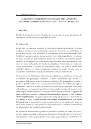
Contents• Introduction to the proposed problem of antennaarrays synthesis• Basic Concepts• Planar arrays• Circular arrays• Results• ConclusionsFinal meeting 20-21 – Warsaw, March 2009General Review of COST296 activities and results2

IntroductionMain objective of COST 296:Develop an increased knowledge of the effects imposed by the ionosphere onpractical radio systems, and for the development and implementation oftechniques to mitigate the deleterious effects of the ionosphere on such systems.In Final Report of COST 284:Geo-stationary satellites were expected to require very large multi-feed reflectorantennas and very versatile arrays and array feeds.The mitigation of the interference can be performed by imposing appropriatednulls on the radiation pattern and by controlling the sidelobe levels.Antenna arrays play an important role in the mitigation of the ionospheric effects.Final meeting 20-21 – Warsaw, March 2009General Review of COST296 activities and results3

Basic ConceptsVxc(x,y,z)dzc 0θxθ =zFourier Relation:φθθyF(βx, βyy, βz)For the farfield, a spatial translation of any sourceonly modifies the produced field in the phase:=∞− ∞∞= ∫ ∫ ∫− ∞(2π)3∞− ∞− 1c ( d)⎯→1ac ( d + d1c(x,y,z)e[ c(x,y,z)]0)F1⎯→j(β x+βx( θ , φ )yy + βaezz)jβ. d0F1dxdydz( θ , φ )βββxyz= β sen( θ )cos( φ )= β sen( θ )sen( φ )= β cos( θ )c(x,y,z)= ∫ ∫ ∫=∞− ∞∞− ∞1(2π)3∞− ∞F(βx, β, β) e[ F(β , β , β )]xyyzz−j(β x+βxyy + βzz)dβxdβydβzFinal meeting 20-21 – Warsaw, March 2009General Review of COST296 activities and results5

Circular ArraysFor patterns with circular symmetry is more appropriated to use circular arrays.The Fourier relation is applied in the same manner as presented previously.However, is more appropriated to deal with polar coordinate system,x = ρ cos( ϕ )y = ρ cos( ϕ )ρ2=x2+y2ββξxy2===ξ cos( ψ )ξ sin( ψ )β2x+β2ySource distribution in polar coordinates systemF(ξ , ψ)=∫∞0∫2π0c(ρ , ϕ ) ej[ ξ cos( ψ ). ρ cos( ϕ ) + ξ sin( ψ ). ρ sin( ϕ ) ]ρ dρdϕArray factor inpolar coordinatessystem=∫∞0∫2π0c(ρ , ϕ ) ejρ ξ cos( ψ − ϕ )ρ dρdϕFinal meeting 20-21 – Warsaw, March 2009General Review of COST296 activities and results7

For radial symmetry of the source distribution and taking into account thatthe array factor isJ01 2πjxcos(α )( x)= ∫ e dα2π0F(ξ )=∫∞0c(ρ ) ⎡⎢⎣∫2π0ejρ ξ cos( ψ − ϕ )dϕ⎤ ρ dρ⎥⎦=2π∫∞0c(ρ ) J0( ρ ξ ) ρ dρThe well-known result for acontinuous disc of uniform current.For discrete arrays, the array factor can be also given byF(βx, βy)=∞∑n=− ∞∞∑m=− ∞c(xn, ym) ej(β xxn+ βyym)Final meeting 20-21 – Warsaw, March 2009General Review of COST296 activities and results8

Comparing with equispaced grids, the periodicity is destroyed in circular arrays.01-5c(x,y)0.80.60.40.2021y (λ)0-1-2 -2-101x(λ)2|F(β x,0)|dB-10-15-20-25-30-30/λ -20/λ -10/λ 0 10/λ 20/λ 30/λ10.80-5β xVisible windowc(x,y)0.60.40.2|F(β x,0)|dB-10-150321y (λ)0-1-2-3-3-2-101x(λ)23-20-25-30-30/λ -20/λ -10/λ 0 10/λ 20/λ 30/λβ xFinal meeting 20-21 – Warsaw, March 2009General Review of COST296 activities and results9

Using the previous changing of variableszθM − 1 N∑m=0m∑− 1n=0[ ξ cos( ψ ). ρ cos( ϕ ) + ξ sin( ψ ). ρ sin( ϕ )]jm nm nF( ξ , ψ ) = c(ρ , ϕ ) emnx2πN mφy=M − 1 N∑m=0m∑− 1n=0cjρmξcos( ψ − ϕ n )( ρm,ϕn)eϕn=2πnNmM – number of ringsN m– number of elements in ring mThis result could be also obtained sampling a continuous source distribution.Final meeting 20-21 – Warsaw, March 2009General Review of COST296 activities and results10

The relation between polar and spherical variables isξ=β2x+β2y=β2sin2( θ )cos2( φ ) +β2sin2( θ )sin2( φ )=βsin( θ )ψ=⎛arctan⎜⎝ββyx⎞⎟⎠=⎡arctan⎢⎣β sin( θ )sin( φ ) ⎤β sin( θ )cos( φ )⎥⎦=φFor an array distribution with radial symmetry,F(ξ )=M − 1 N∑m=0m∑− 1n=0c(ρm, ϕn)∞∑k = − ∞jkJk( ρmξ ) e⎛jk⎜ ψ −⎝2πNm⎞n⎟⎠ejρξ cos( ψ − ϕ )mn=∑ ∞k = − ∞jkJk( ρmξ ) ejk ( ψ − ϕ )n==M − 1∑m=0M − 1∑m=0c(ρNmm)c(ρ∞∑k = − ∞m)jk∞∑Jp=− ∞kJ( ρNmmpξ ) e( ρmjkψξ ) eNm∑− 1n=0jNme2π− j knNm⎛ πp⎜ψ +⎝ 2⎞⎟⎠Usually, few terms of p are enough toobtain a good approximation of thearrays factor.Final meeting 20-21 – Warsaw, March 2009General Review of COST296 activities and results11

Fist terms of the summation:1ρ = 0. 5λ0.50ρ =λ-0.510.500 2/λ 4/λJ 0(ρξ)6/λ 8/λ 10/λ 12/λ 14/λ 16/λ 18/λ 20/λJ N(ρξ)J 2N(ρξ)J 3N(ρξ)-0.50 2/λ 4/λ6/λ 8/λ 10/λ 12/λ 14/λ 16/λ 18/λ 20/λ10.5ρ = 1. 5λ0-0.50 2/λ 4/λ6/λ 8/λ 10/λ 12/λ 14/λ 16/λ 18/λ 20/λFinal meeting 20-21 – Warsaw, March 2009General Review of COST296 activities and results12

Source distribution for discrete circular array,c(ρm, ϕn) ==1(2π)1(2π)22∫∫∞0∞0∫∫2π02π0F(ξ , ψF(ξ , ψ) e) ej[ ξ cos( ψ ). ρ cos( ϕ ) + ξ sin( ψ ). ρ sin( ϕ ) ]jρmmξ cos( ψ − ϕnξ dξdψFor those cases where an independence of ψ exists,)nmnξ dξdψc(ρm)==1(2π)12π∫∞02∫∞0F(ξ ) ⎡⎢⎣F(ξ ) J0∫( ρ2π0mejρmξ ) ξ dξξ cos( ψ − ϕn)dψ⎤ξdξ⎥⎦resulting in the Hankel transform of zero order.F(q)=f ( r)=2π12π∫∫∞0∞0f ( r)J0F(q)J( qr)rdr0( qr)qdqFinal meeting 20-21 – Warsaw, March 2009General Review of COST296 activities and results13

ResultsRectangular array:N=9d=0.5λ81 elementsUniform|F(β x,β y)|dB0dB-10-20-30-40Imposing the peaks amplitude/λβ y/λβ x/λ-50-6/λ -4/λ -2/λ 0 2/λ 4/λ 6/λSLL=-13 dBVisible window0|F(β x,β y)|dB-10-20-30-40/λβ y/λ/λ/λ/λβ x/λ/λ/λ-50-6/λ -4/λ -2/λ 0 2/λ 4/λ 6/λSLL=-30 dBFinal meeting 20-21 – Warsaw, March 2009General Review of COST296 activities and results14

Circular array:M=6N 1=6; N 2=12; N 3=18; N 4=24; N 5=20d=0.5λ between rings81 elementsUniform0- 1 0- 2 0Visible window- 3 0- 4 0|F(β x,β y)|dB- 5 0- 1 0 /λ - 8 /λ - 6 /λ - 4 /λ - 2 /λ 0 2 /λ 4 /λ 6 /λ 8 /λ 1 0 /λSLL=-18.5 dB/λ/λβ y/λ /λβ xFinal meeting 20-21 – Warsaw, March 2009General Review of COST296 activities and results15

Since the desired array factor does not depends of φ,M=6⎧ 1 ξ < 1.3N 1=6; N 2=12; N 3=18; N 4=24; N 5=20 F(ξ ) = ⎨⎩ 0 otherwised=0.5λ between rings81 elements1c( ρ ) = ∫ ∞mF(ξ ) J0( ρmξ) ξ dξ2π0Current in each ring:ρ : 1ρρρρρ012345: 0.95: 0.80: 0.59: 0.36: 0.150Visible window- 1 0- 2 0|F(β x,β y)|dB- 3 0- 4 0/λ- 5 0- 1 0 /λ - 8 /λ - 6 /λ - 4 /λ - 2 /λ 0 2 /λ 4 /λ 6 /λ 8 /λ 1 0 /λ/λSLL=-31.5 dBβ y/λ /λβ xFinal meeting 20-21 – Warsaw, March 2009General Review of COST296 activities and results16

Source distributions:Rectangular arrayCircular array110.8|c(x,y)|0.5|c(x,y)|0.60.40210y(λ)-1-2-2-1.5 -1 -0.5 0 0.5 1 1.5 2x(λ)0.203210-1-2-3-3-2-110x(λ)The feed system of the circular array is simpler than the one of the rectangulargrid since several elements have the same excitation.y(λ)23Final meeting 20-21 – Warsaw, March 2009General Review of COST296 activities and results17

Conclusions• The Fourier Relation method was applied to circular arrays in order tocontrol the radiation pattern.• Comparing with rectangular arrays, the uniform source distributionpermits lower sidelobe levels.• As it was demonstrated, lower sidelobes can be imposed onlycontrolling the source distribution between rings. In each ring thedistribution is uniform whilst for rectangular arrays usually it isnecessary to control the value of all elements.Final meeting 20-21 – Warsaw, March 2009General Review of COST296 activities and results18