Bayesian analysis of ordinal survey data using the Dirichlet process ...

More documents

Recommendations

Info

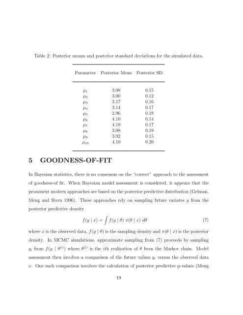
agreement between the model based on the five-point scale and the collapsed model basedon the three-point scale. Of course, we should not expect perfect agreement, especiallyon the b-parameter (extremism), since it is difficult to be characterized as extreme whenthere are only three possible responses.4.2 Simulated DataSeveral simulation studies were carried out to investigate the model. We report on onesuch simulation. A dataset corresponding to n = 150 subjects with m = 10 questions wassimulated using R code. In this example, the mean vector µ = (3, 3, 3, 3, 3, 4, 4, 4, 4, 4) ′and variance covariance matrix Σ = (σ ij ) with σ ii = 4 and σ ij = 2 for i ≠ j were used togenerate the latent matrix Z. The personality parameters a i and b i were set according to(a i , b i ) = (0.0, 1.0) for the first 75 subjects and (a i , b i ) = (0.2, 0.8) for the remaining 75subjects. Having generated Z as described, we then obtained Y via (4) and then obtainedthe observed data matrix X using the cut-point model (1).The model was fit using WinBUGS software where 1000 iterations were used for burnin.The posterior statistics in Table 2 were based on 4000 iterations. We observe that theposterior means of the mean vector are in rough agreement with the true µ. The posteriormeans of Σ are also consistent with the underlying values. The level of agreement is highbecause we have many subjects (n = 150) relative to questions (m = 10). The level ofagreement improved as we increased the number of respondents n.In another simulation, we considered large m (number of survey questions) relative ton (number of subjects). As anticipated, the posterior means of the personality parameters(a i , b i ) were in agreement with the true model parameters, i = 1, . . . , n.18
Table 2: Posterior means and posterior standard deviations for the simulated data.Parameter Posterior Mean Posterior SDµ 1 3.08 0.15µ 2 3.00 0.12µ 3 3.17 0.16µ 4 3.14 0.17µ 5 2.96 0.18µ 6 4.10 0.14µ 7 4.19 0.17µ 8 3.98 0.19µ 9 3.92 0.15µ 10 4.10 0.205 GOODNESS-OF-FITIn Bayesian statistics, there is no consensus on the “correct” approach to the assessmentof goodness-of fit. When Bayesian model assessment is considered, it appears that theprominent modern approaches are based on the posterior predictive distribution (Gelman,Meng and Stern 1996). These approaches rely on sampling future variates y from theposterior predictive density∫f(y | x) = f(y | θ) π(θ | x) dθ (7)where x is the observed data, f(y | θ) is the sampling density and π(θ | x) is the posteriordensity. In MCMC simulations, approximate sampling from (7) proceeds by samplingy i from f(y | θ (i) ) where θ (i) is the ith realization of θ from the Markov chain. Modelassessment then involves a comparison of the future values y i versus the observed datax. One such comparison involves the calculation of posterior predictive p-values (Meng19
Page 1 and 2: Bayesian Analysis of Ordinal Survey
Page 3 and 4: survey where there is a respondent
Page 5 and 6: validity of the model. The proposed
Page 7 and 8: and 4’s. We instead consider a st
Page 9 and 10: our rationale for the Uniform(0, 6)
Page 11 and 12: For programming in WinBUGS, the Set
Page 13 and 14: Markov chain simulations. The resul
Page 15 and 16: Table 1: Posterior means and poster
Page 17: our model gave D = 891. In both the
Page 21 and 22: To provide a more stringent test, w
Page 23 and 24: Brooks, S. P. and Gelman, A. (1997)
Page 25 and 26: Parducci, A. (1965). “Category ju
Page 27 and 28: proportion0.00 0.02 0.04 0.06 0.08
Page 29 and 30: elative frequency0.0 0.1 0.2 0.3●

Bayesian analysis of ordinal survey data using the Dirichlet process ...

You also want an ePaper? Increase the reach of your titles

Delete template?

Save as template?