Bayesian analysis of ordinal survey data using the Dirichlet process ...

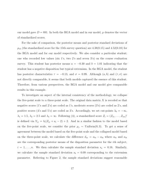
our model gave D = 891. In both the RGA model and in our model, µ denotes the vectorof standardized scores.For the sake of comparison, the posterior means and posterior standard deviations ofµ 15 (the standardized score for the 15th survey question) are 4.38(0.15) and 4.52(0.18) forthe RGA model and for our model respectively. We also consider a particular student;one who recorded low values (six 1’s, two 2’s and seven 3’s) on the course evaluationsurvey. This student has posterior means a = −0.30 and b = 1.01 indicating that thestudent has a negative disposition but typical extremism. In the RGA model, the studenthas posterior characteristics τ = −0.13, and σ = 0.99. Although (a, b) and (τ, σ) arenot directly comparable, it seems that both models captured the essence of this student.Therefore, from various perspectives, the RGA model and our model give comparableresults in this example.To investigate an aspect of the internal consistency of the methodology, we collapsethe five-point scale to a three-point scale. The original data matrix X is recoded so thatnegative scores (1’s and 2’s) are coded as 1’s, moderate scores (3’s) are coded as 2’s, andpositive scores (4’s and 5’s) are coded as 3’s. Accordingly, we set cut-points λ 0 = −∞,λ 1 = 1.5, λ 2 = 2.5 and λ 3 = ∞. Following (4), a standardized score Z i = (Z i1 , . . . , Z im ) ′is defined via Y ij = b i (Z ij + a i − 2) + 2. And in a similar fashion to the model basedon the five-point scale, we consider the prior µ j ∼ Uniform(0, 3). To get a sense ofagreement between the model based on the five-point scale and the collapsed model basedon the three-point scale, we calculate the difference d ai = a 5i − a 3i where a 5i and a 3iare the corresponding posterior means of the disposition parameter for the ith subject,i = 1, . . . , n. We then calculate the sample standard deviation s a = 0.16. Similarly,we calculate the sample standard deviation s b = 0.09 corresponding to the extremismparameter. Referring to Figure 2, the sample standard deviations suggest reasonable17