Bayesian analysis of ordinal survey data using the Dirichlet process ...

Bayesian Analysis of Ordinal Survey Data using theDirichlet Process to Account for RespondentPersonality TraitsSaman Muthukumarana and Tim B. Swartz ∗AbstractThis paper presents a Bayesian latent variable model used to analyze ordinal responsesurvey data by taking into account the characteristics of respondents. Theordinal response data are viewed as multivariate responses arising from continuouslatent variables with known cut-points. Each respondent is characterized bytwo parameters that have a Dirichlet process as their joint prior distribution. Theproposed mechanism adjusts for classes of personalities. The model is applied tostudent survey data in course evaluations. Goodness-of-fit (gof) procedures are developedfor assessing the validity of the model. The proposed gof procedures aresimple, intuitive and do not seem to be a part of current Bayesian practice.Keywords : Dirichlet process, Goodness-of-fit, latent variables, MCMC, WinBUGS.∗ Saman Muthukumarana is Assistant Professor, Department of Statistics, University of Manitoba,Winnipeg Manitoba, Canada R3T2N2. Tim Swartz is Professor, Department of Statistics and ActuarialScience, Simon Fraser University, 8888 University Drive, Burnaby British Columbia, Canada V5A1S6.Both authors have been partially supported by research grants from the Natural Sciences and EngineeringResearch Council of Canada. The authors thank two anonymous reviewers whose comments led to animprovement in the manuscript.1

1 INTRODUCTIONFor the sake of convenience, many surveys consist of ordinal data, often collected on afive-point scale. For example, in a typical course evaluation survey, a student may expresshis view concerning an aspect of the course from a set of five alternatives: 1-poor,2-satisfactory, 3-good, 4-very good, and 5-excellent. Sometimes five-point scales havealternative interpretations. For example, the symmetric Likert scale measures a respondent’slevel of agreement with a statement according to the correspondence: 1-stronglydisagree, 2-disagree, 3-neither agree nor disagree, 4-agree, and 5-strongly agree. Studentfeedback on course evaluation surveys represents a modern approach for measuring quality.Nowadays, a growing number of websites use student feedback as their main performanceindicator in teaching evaluations. As an example, http://www.ratemyprofessors.com/rate over one million professors based on student feedback on a five-point ordinal scale.The scenario is similar in customer satisfaction surveys and social science surveys.The simplest method of summarizing ordinal response data is to report the meanscorresponding to the ordinal scores for each survey question. At a slightly higher level ofstatistical sophistication, standard ANOVA methods may be applied to the ordinal scoresby treating the data as continuous. However, the standard models for the analysis ofordinal data are logistic and loglinear models (Agresti 2010, McCullagh 1980 and Goodmann1979). These models correctly take into account the true measurement scales forordinal data and permit the use of statistical inference procedures for assessing populationcharacteristics. An overview of the methodologies for ordered categorical data is given byLiu and Agresti (2005).The approach in this paper is Bayesian and considers an aspect of ordinal survey datathat is sometimes overlooked. It is widely recognized that respondents may have differingpersonalities. For example, consider a company which conducts a customer satisfaction2

survey where there is a respondent with a negative attitude. The respondent may completethe survey with a preponderance of responses in the 1-2 range. In this case, a response of1 may not truly represent terrible performance on the part of the company. The responsemay reflect more on the disposition of the individual than on the performance of thecompany. As another example of an atypical personality, consider an individual who onlyprovides extreme responses of 1’s and 5’s. It would be useful if statistical analyses couldadjust for personalities. This is the motivation of the paper, and the tool which we use toaccount for personalities is the Dirichlet process, first introduced by Ferguson (1973). As aby-product of the proposed methodology, we attempt to identify areas (survey questions)where performance has been poor or exceptional. In addition, we attempt to identifyquestions that are highly correlated. Clearly, surveyors desire accurate responses and byidentifying highly correlated questions, it allows surveyors to remove redundant questionsfrom the survey which in turn reduces fatigue on the part of the respondents.Our paper is not the first Bayesian paper to consider this problem. AlternativeBayesian approaches include Johnson (1996), Johnson (2003), Dolnicar and Grun (2007),Rossi, Gilula and Allenby (2001), Kottas, Mueller and Quintana (2005), Javaras andRipley (2007) and Emons (2008). Johnson (2003) uses a hierachical ordinal regressionmodel with heterogenious thresholds structure. Dolnicar and Grun (2007) use a ANOVAapproach to assess the inter-cultural differences in responses. Rossi, Gilula and Allenby(2001) address nonidentifiability and parsimony by imposing various complex constraintson the unknown cut-points. Kottas, Mueller and Quintana (2005) propose a nonparametricBayesian approach to model multivariate ordinal data recorded in contingency tables.One of the main features of this paper is that there is a mechanism to cluster subjectsbased on personalities. Most importantly, in our approach, clustering takes place as apart of the model and data determine the clustering structure. Often, clustering is done3

in a post hoc fashion, following some fitting procedure.In addition to the methodological contribution provided in this paper, issues related toscaling are also considered. Not only does the approach attempt to remove idiosyncraticscaling, assumptions are made about the manner in which individuals transform latentcontinuous scores to discrete scores. There is a considerable literature on the psychologyof survey response, the impact of survey question format, the effect of scales, etc. Fora brief introduction to some of these topics, the reader is referred to Tourangeau et al.(2000), Fanning (2005) and Dawes (2008). For an introduction to the analysis of ordinaldata in the applied fields of education and medicine, the reader is referred to Cohen,Manion and Morrison (2007), and Forrest and Andersen (1986) respectively.In section 2, we provide a detailed development of the Bayesian latent variable modelproposed in the paper. The model assumes that ordinal response data arise from continuouslatent variables with known cut-points. Furthermore, each respondent is characterizedby two parameters that have a Dirichlet process as their joint prior distribution.The mechanism adjusts for classes of personalities leading to standardized scores for respondents.Prior distributions are defined on the model parameters. We provide detailsabout nonidentiability in our model and we overcome nonidentifiability issues by assigningsuitable prior distributions. Computation is discussed in section 3. As the resulting posteriordistribution is complex and high-dimensional, we approximate posterior summarystatistics which describe key features in the model. In particular, posterior expectationsare obtained via MCMC methods using WinBUGS software (Spiegelhalter, Thomas andBest 2003). In section 4, the model is applied to actual student survey data obtained incourse evaluations. A comparison is made with an analysis based on the methodology ofRossi, Gilula and Allenby (2001). We then demonstrate the reliability of the approachvia simulation. In section 5, goodness-of-fit procedures are developed for assessing the4

validity of the model. The proposed procedures are simple, intuitive and do not seem tobe a part of current Bayesian practice. We conclude with a short discussion in section 6.2 MODEL DEVELOPMENTConsider a survey where the observed data are described by a matrix X : (n × m) whoseentries X ij are the ordinal responses. The n rows of X correspond to the individuals whoare surveyed and the m columns refer to the survey questions. Without loss of generality,we assume that the responses are taken on a five-point scale.We assume that the discrete response X ij of individual i to survey question j arisesfrom an underlying continuous variable Y ij . We consider a cut-point model which convertsthe latent variable Y ij to the observed X ij as follows:X ij = 1 ⇐⇒ λ 0 < Y ij ≤ λ 1X ij = 2 ⇐⇒ λ 1 < Y ij ≤ λ 2X ij = 3 ⇐⇒ λ 2 < Y ij ≤ λ 3(1)X ij = 4 ⇐⇒ λ 3 < Y ij ≤ λ 4X ij = 5 ⇐⇒ λ 4 < Y ij ≤ λ 5Up until this point, our approach is identical to that of Rossi, Gilula and Allenby(2001). Our approach now deviates as we assume that the cut-points are known and aregiven by λ 0 = −∞, λ 1 = 1.5, λ 2 = 2.5, λ 3 = 3.5, λ 4 = 4.5 and λ 5 = ∞. We suggestthat the chosen cut-points correspond to the way that respondents actually think. Whenasked to supply information on a five-point scale, we hypothesize that respondents makeassessments on the continuum where the values 1.0, . . . , 5.0 have precise meaning. Therespondents then implicitly round the continuous score to the nearest of the five integers.Although our methodology can be modified using unknown cut-points, the estimation of5

cut-points introduces difficulties involving nonidentifiability. Rossi, Gilula and Allenby(2001) address nonidentifiability and parsimony by imposing numerous constraints on thecut-points.It is interesting to compare our rationale for the Y ij → X ij transformation with therange-frequency model proposed by Parducci (1965). The range principle suggests that arespondent uses extreme stimuli to fix the interpretation of endpoints on a discrete scale,and these endpoints provide reference for intermediate scale values. The principle isconsistent with our transformation rationale as rounding is a subsequent step to markinglatent variables on a continuum. On the other hand, the frequency principle appears tobe violated as there is no reason to expect constant frequencies between scales values.This departure may be expected on the grounds of a reference point effect where Likertscale values, for example, have specific meanings. The frequency-range model and variousdepartures from the model are discussed in Tourangeau et al. (2000).Using the notation Y i = (Y i1 , . . . , Y im ) ′ , Rossi, Gilula and Allenby (2001) considerY i ∼ Normal(µ + τ i 1, σi 2 Σ) (2)for i = 1, . . . , n where τ i and σ i are respondent-specific parameters used to address scaleusage heterogeneity. For example, a large τ i and small σ i > 0 characterize a respondentwho uses the top end of the scale. Further, the model (2) implies a standardized response(Y ij −µ j −τ i )/σ i through which the correlation between survey questions may be assessed.A consequence of the model is that correlation inferences between survey questions maydiffer considerably when scale usage characteristics are considered.Although (2) contains many of the features we desire, it cannot, for example, adequatelymodel an individual whose responses are mostly intermediate values such as 2’s6

and 4’s. We instead consider a structure that has similarities to (2). We proposeY i ∼ Normal(b i (µ + a i 1 − 31) + 31, b 2 i Σ) (3)where we adjust for personalities via a “pure” or standardized score for the ith individualgiven by Z i = (Z i1 , . . . , Z im ) ′ ∼ Normal(µ, Σ) such thatY ij = b i (Z ij + a i − 3) + 3 (4)for i = 1, . . . , n, j = 1, . . . , m.It is (4) that provides an interpretation for the latent responses Z i and Y i , and forthe parameters a i and b i corresponding to the ith individual. We observe that Z i is astandardized latent score which is independent and identically distributed across respondents.The vector µ corresponds to the mean response of standardized scores over thepopulation of respondents, and the matrix Σ describes the variability of these scores andthe correlation between survey questions. The latent score Y i is obtained from Z i via (4)where Y i includes the personality characteristics (a i , b i ) of the ith respondent. Unlike theZ i , we note that the Y i in (3) are not identically distributed. Therefore, the learning of(a i , b i ) can be thought of as a denoising method where the pure response Z i is derivedfrom the noisy Y i which includes personality traits.For an interpretation of the disposition parameter a i ∈ R in (4), it is initially helpfulto consider a i conditional on b i = 1. In this case, when a i = 0, the ith respondent hasa neutral disposition and the latent response Y ij is equal to the standardized score Z ij .When a i > 0 (a i < 0), the ith respondent has a positive (negative) attitude since Z ij isadjusted by a i to give Y ij .For an interpretation of the extremism parameter b i > 0 in (4), it is helpful to considerb i conditional on a i = 0. In this case, when b i > 1, the amount by which Z ij exceeds 3.0is magnified and is added to 3.0 and gives a more extreme result towards the tails on the7

five-point scale. When 0 ≤ b i < 1, the extremism parameter has the effect of pulling thelatent response Y ij closer to the middle. A respondent whose b i ≈ 0 might be described asmoderate and we impose the constraint b i > 0 to avoid nonidentifiability. Note that theparameter σ i in (2) addresses variability which is somewhat different from our concept ofextremism.To provide a little more clarity, when Z ij + a i − 3 > 0, the ith respondent is positivelyinclined towards survey question j. When Z ij + a i − 3 < 0, the i-th respondent isnegatively inclined towards survey question j. The quantity Z ij + a i − 3 is then scaled byb i to account for extremism on the part of the i-th respondent. The personality differentialb i (Z ij + a i − 3) is then added to 3 to yield the latent variable Y ij . Note that whereas azero score for b i (Z ij + a i − 3) represents ambivalence (neither agree nor disagree in theLikert setting), Y ij = 3 represents ambivalence in the latent variable. Having adjusted forrespondent personalities, we are interested in the average response µ for the m questionsand the corresponding correlation structure Σ. We recognize that not all individuals sharethe same temperment. The i-th respondent is characterized by the parameters a i and b iwhere a i is the disposition parameter and b i is the extremism parameter.As the proposed approach is Bayesian, prior distributions are required for the modelparameters in (3). Specifically, we assign moderately diffuse priorsΣ −1 ∼ Wishart m (I, m)µ j ∼ Uniform(0, 6)where the components of µ = (µ 1 , . . . , µ m ) ′ are apriori independent. The Wishart distributionis the standard and conjugate prior distribution for the inverse covariance matrixin normal models (Bernardo and Smith 1994) where the identity matrix and degrees offreedom parameter m are convenient choices in the absence of subjective prior information.Regarding the parameters µ j , although it is tempting to assign flat improper priors,8

our rationale for the Uniform(0, 6) prior distribution is based on the observed responseX ij constrained to the five-point scale. It is thought that X ij represents the rounded scoreof the continuous latent variable Y ij whose mean is µ j when b i = 1 and a i = 0. For thepersonality parameters a i and b i , the prior assignment is based on the supposition thatthere are classes of personalities. We therefore consider the Dirichlet process(a i , b i ) ′ iid ∼ GG ∼ DP(α, tr-Normal 2 (µ G , Σ G ))(5)for i = 1, . . . , n. The specification in (5) states that (a i , b i ) arises from a distribution Gbut G itself arises from a distribution of distributions known as the Dirichlet process. TheDirichlet process in (5) consists of the concentration parameter α and baseline distributiontr-Normal 2 (µ G , Σ G )) where tr-Normal refers to the truncated bivariate Normal whosesecond component b i is constrained to be positive. The baseline distribution serves as aninitial guess of the distribution of (a i , b i ) and the concentration parameter determines ourconfidence in the baseline distribution with large values of α > 0 corresponding to greaterdegrees of belief. Prior distributions can be assigned to the hyperparameters in (5). Ouranalyses involving course evaluation surveys on a five-point scale give sensible resultswith α ∼ Uniform(0.4, 10) (Ohlssen, Sharples and Spiegelhalter, 2007), µ G = (0, 1) ′ andΣ G = (σ ij ) where σ 11 = 1.0, σ 22 = 0.5 and σ ij = 0 for i ≠ j. Note that the choice of1.0 and 0.5 are sufficiently diffuse in the range of parameters a i and b i . The key aspectof the Dirichlet process in our application is that the personality parameters (a i , b i ) havesupport on a discrete space and this enables the clustering of personality types. Anadvantage of the Dirichlet process approach is that clustering is implicitly carried out inthe framework of the model and the number of component clusters need not be specified inadvance. Once a theoretical curiousity, the Dirichlet process and its extensions are findingdiverse application areas in nonparametric modelling (e.g. Qi, Paisley and Carin 2007,9

Dunson and Gelfand 2009, Gill and Casella 2009). The nonparametric prior specificationin our model and the associated clustering of subjects provides another essential differencebetween our approach and that of Rossi, Gilula and Allenby (2001).3 COMPUTATIONThe model described in section 2 is generally referred to as a Dirichlet process mixturemodel, and various Markov chain methodologies have been developed to facilitatesampling-based analyses (Neal 2000).sophistication on the part of the programmer.However, these algorithms require considerableA goal in this paper is to simplify the programming aspect of the analysis by carryingout computations in WinBUGS. The basic idea behind WinBUGS is that the programmerneed only specify the statistical model, the prior and the data. The Markov chaincalculations are done in the background whereby the user is then supplied with Markovchain output. Markov chain output is then conveniently averaged to give approximationsof posterior means.To implement the analysis of our model in WinBUGS, we make use of the constructivedefinition of the Dirichlet process given by Sethuraman (1994). The definition is knownas the stick breaking representation, and in the context of our problem, it is given asfollows: Generate a set of iid atoms (a ∗ i , b ∗ i ) from tr-Normal 2 (µ G , Σ G ) and generate a setof weights w i = y i∏ i−1j=1(1 − y j ) where the y i are iid with y i ∼ Beta(1, α) for i = 1, . . . , ∞.Thenwhere δ (a ∗i ,b ∗ i ) is the point mass at (a ∗ i , b ∗ i ).∞∑G = w i δ (a ∗i ,b ∗ i ) (6)i=110

For programming in WinBUGS, the Sethurman (1994) construction is most useful asit allows us to approximately specify the prior. We see that the stick breaking mechanismcreates smaller and smaller weights w i . This suggests that at a certain point we cantruncate the sum (6) and obtain a reasonable approximation to G (Muliere and Tardella1998). Ishwaran and Zarepour (2002) suggest that the number of truncation points be nwhen the sample size is small and √ n when the sample size is large. The stick breakingconstruction clearly shows that a generated G is a discrete probability distribution whichimplies that there is non-negligible probability that (a i , b i )’s generated from the same Ghave the same value. This facilitates the clustering of personalities in ordinal survey data.We note that the original definition of the Dirichlet process (Ferguson 1973) does notprovide a WinBUGS-tractable expression for the prior.4 EXAMPLES4.1 Course Evaluation Survey DataThe proposed model is fit to data obtained from teaching and course evaluations in theDepartment of Statistics and Actuarial Science at Simon Fraser University (SFU). Thestandard questionnaire at SFU contains m = 15 questions with responses on a five-pointscale ranging from 1 (a very negative response) to 5 (a very positive response) wherethe specific interpretation of responses are question dependent. The survey questions aregiven as follows:1. The course text or supplementary material was2. I would rate this course as3. The assignments and lectures were4. The assignments and exams were on the whole11

5. The marking scheme was on the whole6. How informative were the lectures7. The Instructor’s organization and preparation were8. The Instructor’s ability to communicate material was9. The Instructor’s interest in the course content appeared to be10. The Instructor’s feedback on my work was11. Questions during class were encouraged12. Was the Instructor accessible for extra help13. Was the Instructor responsive to complaints/suggestions14. Overall, the Instructor’s attitude towards students was15. I would rate the Instructor’s teaching ability asData were collected from n = 75 students pertaining to an introductory Statisticscourse. Posterior means and standard deviations corresponding to the parameter µ aregiven in Table 1. These are based on a MCMC simulation using WinBUGS with aburn-in period of 1000 iterations followed by 4000 iterations, taking roughly 2 hours ofcomputation on a personal computer. The WinBUGS code is provided in the Appendix.The highest posterior mean was recorded for the 9th question which asked about “theInstructor’s interest in the course material”. The smallest mean was recorded for the10th question which asked about “the Instructor’s feedback on work”. These resultsare consistent with past surveys taken in the same course with the same Instructor. Inparticular, the Instructor does not grade assignments and this yields some criticisms fromthe students. Note that the posterior standard deviations are sufficiently small such thatwe can sensibly discuss the posterior means.To investigate the clustering effect, we recorded the number of clusters in each of the12

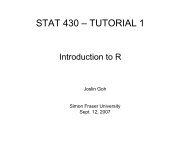
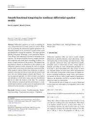
Markov chain simulations. The resulting histogram is given in Figure 1. We observe thatthere are quite a few clusters, and there is considerable uncertainty about the number ofclusters. More specifically, the number of clusters appears roughly uniform between 3 and18, with approximately 10 clusters on average. This implies that there is a substantialnumber of personality types amongst the n = 75 students. The clustering effect is corroboratedin Figure 2 where we provide a plot of the posterior means of the (a i , b i ) pairs.By looking closely along both vertical and horizontal strips, there are approximately 10classes of personalities, some of which do not differ greatly. In Figure 2, the clustering ismore difficult to distinguish with respect to the disposition parameter a, suggesting morevariability in a than in b. We observe that roughly 50% of the a i ’s are greater than 0.0,and roughly 50% of the b i ’s are greater than 1.0.For small values of b, the corresponding students tend to have responses which areoften the same, and this may be due to a desire to finish the questionnaire as quicklyas possible. With b = 1.0, the interpretation is that these students do not distort theirresponses in an inflationary/deflationary sense, and there are roughly 20 students of thistype. For large values of b, the corresponding students inflate their responses; they makeharsher decisions near both ends of the scale (1’s and 5’s).Note that one of the respondents provided a score of 5.0 for all m = 15 questions. Itturns out that the corresponding posterior mean of (a i , b i ) for this student was (0.36, 1.09).Based on an average posterior response ¯µ = 4.1, this student’s mean latent Y-score is1.09(¯µ + 0.36 − 3) + 3 = 4.59 which rounds to a respondent X-score of 5.0 accordingto the cut-point model (1). This provides some evidence that the (a i , b i ) parametersare estimated sensibly. For this student, we note that the variance 1.09Σ of the latentresponse Y i which includes personality traits exceeds the variance Σ of the standardizedresponse Z i . This is because the student in question is “extreme”, and has the capacity13

for extreme responses of 0’s and 5’s. This case highlights a distinction between our notionof extremism and variability.As another example of the adjustment made for personalities, the smallest posteriormean for the disposition parameter corresponds to a i = −0.30 which was recorded for astudent with an average observed response ¯X i = 2.06 over all m = 15 questions. Thisstudent has a corresponding extremism parameter b = 1.01. The question arises asto whether 2.06 is a measurement that should be taken at face value when the averageresponse and standard deviation over all students are 3.89 and 1.02 respectively. It appearsthat 2.06 is an extreme score lying 1.8 standard deviations from the mean. However, whenwe adjust for the personality of the student via (4), we obtain Y i = 1.01(Z i − 0.301 −31) + 31 ≈ Z i − 0.31. This implies that the standardized but latent response Z i is largerthan Y i . The student has a negative disposition, and when we account for the negativedisposition, the de-noised score Z i is not as extreme as the raw data X i .It is also instructive to look at the posterior mean of the variance-covariance matrixΣ which describes the relationships amongst the m = 15 survey questions. The largestcorrelation 0.63 occurred between survey questions 14 and 15. This is consistent withour intuition and personal teaching experience whereby students think highly of theirinstructors when they believe that their instructors care about them. The second highestcorrelation 0.57 occurred between survey questions 6 and 7 which is also believable fromthe view that learning is best achieved when material is clearly presented. However, weemphasize that the elimination of questions on the basis of redundancy should not bedone solely on the basis of high correlations. In addition to high correlations, we shouldalso have similar posterior means. With the estimated posterior means µ 14 = 4.57 andµ 15 = 4.52, SFU may feel comfortable in dropping either question 14 or question 15 fromthe survey. Furthermore, we note that there were no negative posterior correlations and14

Table 1: Posterior means and posterior standard deviations for the SFU survey data.Parameter Posterior Mean Posterior SDµ 1 3.69 0.19µ 2 3.53 0.15µ 3 4.04 0.18µ 4 3.45 0.17µ 5 3.85 0.17µ 6 4.54 0.19µ 7 4.33 0.18µ 8 4.41 0.17µ 9 4.78 0.15µ 10 3.23 0.17µ 11 4.51 0.19µ 12 4.01 0.18µ 13 4.11 0.17µ 14 4.57 0.19µ 15 4.52 0.18¯µ 4.10the minimum correlation 0.11 occurred between question 1 and question 13. Our intuitionaccordingly suggests that these two questions are independent. For comparison, we havealso calculated the sample correlation matrix based on the raw scores X. The values alignwith the posterior mean of Σ. For example, the smallest sample correlation is 0.10 andthis is observed between question 1 and question 13. The largest sample correlation is0.78 and this occurs between questions 14 and 15.It is good statistical practice to look at various plots related to the MCMC simulation.Trace plots for the parameters appear to stabilize immediately and hence provide no15

indication of lack of convergence in the Markov chain. Furthermore, autocorrelation plotsappear to dampen quickly. This provides added evidence of the convergence of the Markovchain and also suggests that it may be appropriate to average Markov chain output asthough the variates are independent. In addition to the diagnostics described, multiplechains were generated to provide further assurance of the reliability of the methods.For example, the Brooks-Gelman-Rubin statistic (Brooks and Gelman 1997) gave noindication of lack of convergence.We now consider the analysis of the SFU survey data using the methodology of RGA(Rossi, Gilula and Allenby 2001). Whereas our model uses known cut-points which convertthe latent variable Y ij to the observed X ij , RGA have cut-points that are determined viaconstraints and a single unknown parameter e. For the RGA analysis, λ i = c + di + ei 2 ,i = 1, . . . , 4, and the constraints ∑ 4i=1 λ i = 12 and ∑ 4i=1 λ 2 i = 41 were imposed suchthat the cut-points are apriori centred about the known cut-points in our model wheree ∼ Uniform(−0.2, 0.2).Fitting the RGA model, we obtained posterior means e = −0.003, λ 1 = 1.50, λ 2 =2.51, λ 3 = 3.51 and λ 4 = 4.48 where we observe that the RGA cut-points are very closeto the fixed cut-points used in our model. To compare the fit of the RGA model withour model using the SFU survey data, we calculated the posterior mean of the diagnosticD = ∑ (y ij − β ij ) 2 where β ij denotes the mean of y ij and the summation is taken overall pairs (i, j) where x ij ≠ 1 and x ij ≠ 5 (see (1)). The restricted summation is imposedsince the RGA model does not impose lower and upper values for y ij , and consequentlysmall/large posterior variates y ij greatly inflate the diagnostic D. The diagnostic D isin the spirit of deviances (McCullagh and Nelder 1989) where y ij denotes the underlyinglatent score in both the RGA model and in our model. In the RGA model (2), β ij = µ j +τ i ,and in our model (3), β ij = b i (µ j + a i − 3) + 3. Whereas the RGA model gave D = 936,16

our model gave D = 891. In both the RGA model and in our model, µ denotes the vectorof standardized scores.For the sake of comparison, the posterior means and posterior standard deviations ofµ 15 (the standardized score for the 15th survey question) are 4.38(0.15) and 4.52(0.18) forthe RGA model and for our model respectively. We also consider a particular student;one who recorded low values (six 1’s, two 2’s and seven 3’s) on the course evaluationsurvey. This student has posterior means a = −0.30 and b = 1.01 indicating that thestudent has a negative disposition but typical extremism. In the RGA model, the studenthas posterior characteristics τ = −0.13, and σ = 0.99. Although (a, b) and (τ, σ) arenot directly comparable, it seems that both models captured the essence of this student.Therefore, from various perspectives, the RGA model and our model give comparableresults in this example.To investigate an aspect of the internal consistency of the methodology, we collapsethe five-point scale to a three-point scale. The original data matrix X is recoded so thatnegative scores (1’s and 2’s) are coded as 1’s, moderate scores (3’s) are coded as 2’s, andpositive scores (4’s and 5’s) are coded as 3’s. Accordingly, we set cut-points λ 0 = −∞,λ 1 = 1.5, λ 2 = 2.5 and λ 3 = ∞. Following (4), a standardized score Z i = (Z i1 , . . . , Z im ) ′is defined via Y ij = b i (Z ij + a i − 2) + 2. And in a similar fashion to the model basedon the five-point scale, we consider the prior µ j ∼ Uniform(0, 3). To get a sense ofagreement between the model based on the five-point scale and the collapsed model basedon the three-point scale, we calculate the difference d ai = a 5i − a 3i where a 5i and a 3iare the corresponding posterior means of the disposition parameter for the ith subject,i = 1, . . . , n. We then calculate the sample standard deviation s a = 0.16. Similarly,we calculate the sample standard deviation s b = 0.09 corresponding to the extremismparameter. Referring to Figure 2, the sample standard deviations suggest reasonable17

agreement between the model based on the five-point scale and the collapsed model basedon the three-point scale. Of course, we should not expect perfect agreement, especiallyon the b-parameter (extremism), since it is difficult to be characterized as extreme whenthere are only three possible responses.4.2 Simulated DataSeveral simulation studies were carried out to investigate the model. We report on onesuch simulation. A dataset corresponding to n = 150 subjects with m = 10 questions wassimulated using R code. In this example, the mean vector µ = (3, 3, 3, 3, 3, 4, 4, 4, 4, 4) ′and variance covariance matrix Σ = (σ ij ) with σ ii = 4 and σ ij = 2 for i ≠ j were used togenerate the latent matrix Z. The personality parameters a i and b i were set according to(a i , b i ) = (0.0, 1.0) for the first 75 subjects and (a i , b i ) = (0.2, 0.8) for the remaining 75subjects. Having generated Z as described, we then obtained Y via (4) and then obtainedthe observed data matrix X using the cut-point model (1).The model was fit using WinBUGS software where 1000 iterations were used for burnin.The posterior statistics in Table 2 were based on 4000 iterations. We observe that theposterior means of the mean vector are in rough agreement with the true µ. The posteriormeans of Σ are also consistent with the underlying values. The level of agreement is highbecause we have many subjects (n = 150) relative to questions (m = 10). The level ofagreement improved as we increased the number of respondents n.In another simulation, we considered large m (number of survey questions) relative ton (number of subjects). As anticipated, the posterior means of the personality parameters(a i , b i ) were in agreement with the true model parameters, i = 1, . . . , n.18

Table 2: Posterior means and posterior standard deviations for the simulated data.Parameter Posterior Mean Posterior SDµ 1 3.08 0.15µ 2 3.00 0.12µ 3 3.17 0.16µ 4 3.14 0.17µ 5 2.96 0.18µ 6 4.10 0.14µ 7 4.19 0.17µ 8 3.98 0.19µ 9 3.92 0.15µ 10 4.10 0.205 GOODNESS-OF-FITIn Bayesian statistics, there is no consensus on the “correct” approach to the assessmentof goodness-of fit. When Bayesian model assessment is considered, it appears that theprominent modern approaches are based on the posterior predictive distribution (Gelman,Meng and Stern 1996). These approaches rely on sampling future variates y from theposterior predictive density∫f(y | x) = f(y | θ) π(θ | x) dθ (7)where x is the observed data, f(y | θ) is the sampling density and π(θ | x) is the posteriordensity. In MCMC simulations, approximate sampling from (7) proceeds by samplingy i from f(y | θ (i) ) where θ (i) is the ith realization of θ from the Markov chain. Modelassessment then involves a comparison of the future values y i versus the observed datax. One such comparison involves the calculation of posterior predictive p-values (Meng19

1994). A major difficulty with posterior predictive methods concerns double use of thedata (Evans 2007). Specifically, the observed data x is used both to fit the model givingrise to the posterior density π(θ | x) and then is used in the comparison of y i versus x. Forthis reason, some authors prefer a cross-validatory approach (Gelfand, Dey and Chang1992) where the data x = (x 1 , x 2 ) are split such that x 1 is used for fitting and x 2 is usedfor validation.We take the view that in assessing a Bayesian model, the entire model ought to beunder consideration, and the entire model consists of both the sampling model of thedata and the prior. We also want a methodology that does not suffer from double use ofthe data. For the models proposed here, we recommend an approach that is similar tothe posterior predictive methods but instead samples “model variates” y from the priorpredictive density∫f(y) = f(y | θ) π(θ) dθ (8)where π(θ) is a proper prior density. This approach was advocated by Box (1980) beforesimulation methods were common. It is not difficult to write R code to simulate y 1 , . . . , y Nfrom the prior predictive density in (8). It is then a matter of deciding how to compare they i ’s against the observed data matrix X. In our application, the data are high dimensional,and we advocate a comparison of “features” that are of direct interest. This is an intuitiveand simple approach which is not part of current statistical practice. For example, onemight compare observed subject means ¯X i = ∑ mj=1 X ij /m with subject means generatedfrom the prior predictive simulation. A simple comparison of these vectors can be easilycarried out through the calculation of Euclidean distances. Naturally, as the priors becomemore diffuse, it becomes less likely to find evidence of model inadequacy. We do not viewthis as a failing of the methodology. Rather, if you really want to detect departures froma model, it is necessary that you have strong prior opinion concerning your model.20

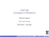
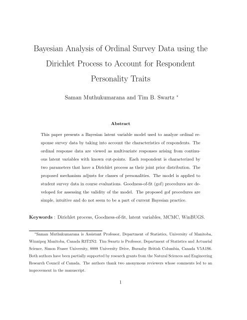
To provide a more stringent test, we consider a modification of our model where subjectivepriors µ j ∼ Uniform(2, 5) and Σ G = 0.01I are introduced. We assess goodness-offit on the SFU data discussed in section 4. With N simulated vectors from the prior predictivedistribution, there are ( N+12 ) Euclidean distances of interest; N of these distancesare between the observed mean vector and the simulated vectors, and the remaining ( N 2 )distances correspond to distances between simulated vectors. These distances are displayedin a histogram with the N = 20 distances highlighted in Figure 3. Since thesedistances appear typical, there is no evidence of lack of fit. In fact, we observe that mostof the Euclidean distances involving observed data lie on the left side of the histogram.This suggests that the most extreme variates arose from the prior-predictive distribution.Clearly, graphical displays for alternative features can also be produced.Another approach to Bayesian goodness-of-fit which appears promising in the contextof the proposed model is due to Johnson (2007). Let θ consist of all model parameters, letX i be the vector of discrete responses for the ith respondent and let β i = b i (µ+a i 1−31)+31denote the mean of the corresponding latent variable Y i , i = 1, . . . , n. Under the “true”θ, we then note that S(X i , θ) = (Y i − β i ) ′ Σ −1 (Y i − β i )/b 2 i is distributed as a Chi-squarevariable with m = 15 degrees of freedom. Following Johnson (2007), S(X i , θ) is pivotalin the sense that its conditional distribution does not depend on θ and there are n = 75values of S(X i , θ) that can be calculated for a given θ. For a single sampled value θ fromthe MCMC simulation, Figure 4 provides a plot of the ordered values of S(X i , θ) versusthe theoretical Chi-square quantiles. The plotted points appear to be roughly scatteredabout the line y = x and hence provide no strong indication of lack of fit.21

6 DISCUSSIONWe have developed a Bayesian latent variable model to analyze ordinal response surveydata. We have also facilitated a clustering mechanism based on personalities. Mostimportantly, clustering takes place as a consequence of Dirichlet process modelling ofthe personality parameters. In a WinBUGS programming environment, the model issuccinctly formulated, and is not complicated by latent variables and missing data.Our model identifies areas where performance has been poor or exceptional in a ordinalsurvey data by investigating standardized parameters. It also allows us to check whethersome questions in a survey are redundant. A goodness-of-fit procedure is advocated thatis based on comparing prior-predictive output versus observed data. The approach isintuitive and is flexible in the sense that one can investigate features which are relevant tothe particular model. Future enhancements may be considered such as including subjectcovariates and handling longitudinal data structures.One of the assumptions in our model concerns the use of fixed cut-points in transformingthe underlying continuous latent responses Y ij to the observed discrete responsesX ij . Although it may have been preferable to allow variable cut-points, we were unableto implement the generalization. Issues of non-identifiablility and model complexity leadto Markov chains which did not achieve practical convergence.7 REFERENCESAgresti, A. (2010). Analysis of Ordinal Categorical Data, Second Edition, Wiley: New York.Bernardo, J.M. and Smith, A.F.M. (1994). Bayesian Theory, Wiley: New York.Box, G. E. (1980). “Sampling and Bayes’ inference in scientific modelling and robustness”(with discussion), Journal of the Royal Statistical Society, Series A, 143, 383–430.22

Brooks, S. P. and Gelman, A. (1997). “Alternative methods for monitoring convergence ofiterative simulations”, Computational and Graphical Statistics, 7, 434–455.Cowen, L., Manion, L. and Morrison, K. (2007). Research Methods in Education, Sixth Edition,Routledge: New York.Dawes, J. (2008). “Do data characteristics change according to the number of scale pointsused? An experiment using 5-point, 7-point and 10-point scales”, International Journalof Market Research, 50, 61-77.Dolnicar, S. and Grun, B. (2007). “Cross-cultural differences in survey response patterns”,International Marketing Review, 24, 127-143.Dunson, D.B. and Gelfand, A.E. (2009). “Bayesian nonparametric functional data analysisthrough density estimation”, Biometrika, 96, 149-162.Emons, W.H.M. (2008). “Nonparametric person-fit analysis of polytomous item scores”, AppliedPsychologial Measurement, 32, 224-247.Evans, M. (2007). Comment on “Bayesian checking of the second levels of hierarchical models”by Bayarri and Castellanos, Statistical Science, 22, 344-348.Fanning, E. (2005). “Formatting a paper-based survey questionnaire: best practices”, PracticalAssessment Research & Evaluation, online: http://pareonline.net/pdf/v10n12.pdf.Ferguson, T.S. (1973). “A Bayesian analysis of some nonparametric problems”, Annals ofStatistics, 1, 209-230.Forrest, M. and Andersen, B. (1986). “Ordinal scale and statistics in medical research”, BritishMedical Journal, 292, 537-538.Gelfand, A. E., Dey, D. K. and Chang, H. (1992). “Model determination using predictive distributionswith implementation via sampling-based methods” (with discussion), In BayesianStatistics 4 (J. M. Bernardo, J. O. Berger, A. P. Dawid & A. F. M. Smith, editors),Oxford: Oxford University Press, 147–167.Gelman, A., Meng, X. L. and Stern, H. S. (1996). “Posterior predictive assessment of modelfitness via realized discrepancies”, Statistica Sinica, 6, 733–807.Gill, J. and Casella, G. (2009). “Nonparametric priors for ordinal Bayesian social sciencemodels: specification and estimation”, Journal of the American Statistical Association,104, 453-464.23

Goodmann, L.A. (1979). “Simple models for the analysis of association in cross-classificationshaving ordered categories”, Journal of the American Statistical Association, 74, 537-552.Ishwaran, H. and Zarepour, M. (2002).Statistica Sinica, 12, 941-963.“Dirichlet prior sieves in finite normal mixtures”,Javaras, K.N. and Ripley, B.D. (2007). “ An ‘unfolding’ latent variable model for Likertattitude data: Drawing inferences adjusted for response style”, Journal of the AmericanStatistical Association, 102, 454-463.Johnson, T.R. (2003). “On the use of heterogeneous thresholds ordinal regression models toaccount for individual differences in response style”, Psychometrika, 68, 563-583.Johnson, V.E. (1996). “On Bayesian analysis of multirater ordinal data: An application toautomated essay grading”, Journal of the American Statistical Association, 91, 42-51.Johnson, V.E. (2007). “Bayesian model assessment using pivotal quantities”, Bayesian Analysis,2, 719-734.Kottas, A., Mueller, P. and Quintana, F. (2005). “Nonparametric Bayesian Modeling forMultivariate Ordinal Data”, Journal of Computational and Graphical Statistics, 14, 610-625.Liu, I. and Agresti, A. (2005). “The analysis of ordered categorical data: An overview and asurvey of recent developments”, Test, 14, 1-73.McCullagh, P. (1980). “Regression models for ordinal data (with discussion)”, Journal of theRoyal Statistical Society, Series B, 42, 109-142.McCullagh, P. and Nelder, J.A. (1989). Generalized Linear Models, Second Edition, Chapmanand Hall: London.Meng, X.L. (1994). “Posterior predictive p-values”, The Annals of Statistics, 22, 1142–1160.Muliere, P. and Tardella, L. (1998). “Approximating distributions of random functionals ofFerguson-Dirichlet priors”, Canadian Journal of Statistics, 26, 283-297.Neal, R.M. (2000). “Markov chain sampling methods for Dirichlet process mixture models”,Journal of Computational and Graphical Statistics, 9, 249-265.Ohlssen, D., Sharples, L.D. and Spiegelhalter, D.J. (2007). “Flexible random-effects modelsusing Bayesian semi-parametric models: applications to institutional comparisons”,Statistics in Medicine, 26, 2088-2112.24

Parducci, A. (1965). “Category judgment: A range-frequency model”, Psychological Review,72, 407-418.Qi, Y., Paisley, J.W. and Carin, L. (2007). “Music analysis using hidden markov mixturemodels” IEEE Transactions in Signal Processing, 55, 5209-5224.Rossi, P.E., Gilula, Z. and Allenby, G.M. (2001). “Overcoming scale usage heterogeneity”,Journal of the American Statistical Association, 96, 20-31.Sethuraman, J. (1994). “A constructive definition of Dirichlet priors”, Statistica Sinica, 4,639-650.Spiegelhalter, D. Thomas, A. and Best, N. (2003). WinBUGS (Version 1.4) User Manual,Cambridge: MRC Biostatistics Unit.Tourangeau, R., Rips, L. and Rasinski, K. (2000). The Psychology of Survey Response, CambridgeUniversity Press: Cambridge.8 APPENDIXWe provide the WinBUGS code used in the analysis of the SFU survey data.model{# cut point model as defined in (1)alpha[1]

{cor[i,j]

proportion0.00 0.02 0.04 0.06 0.08 0.101 2 3 4 5 6 7 8 9 10 11 12 13 14 15 16 17 18 19 20number of clustersFigure 1: Histogram of the number of clusters for the SFU survey data.27

●b0.85 0.90 0.95 1.00 1.05 1.10 1.15●●●●●●●● ● ●●●●● ●●● ●● ●● ● ●●● ●●●●●●● ● ● ● ●●● ●● ● ●● ● ●●●●● ●●● ●●●●● ●●●●●●−0.3 −0.2 −0.1 0.0 0.1 0.2 0.3aFigure 2: Plot of the posterior means of the personality parameters (a i , b i ) for the SFUsurvey data.28

elative frequency0.0 0.1 0.2 0.3●●●● ● ●●●●●● ● ●●9 10 11 12 13 14Euclidean distancesFigure 3: Histogram corresponding to the ( N+12 )= 210 Euclidean distances with respectto the prior-predictive check for the SFU survey data.29

●quantiles of S0 10 20 30 40●● ●● ●● ●●●●● ●●●●●●●●●●●●● ●● ●● ●● ●●● ●●●●●●●● ●●●●● ●● ● ● ● ● ●5 10 15 20 25 30 35theoretical Chi−square quantilesFigure 4: Q-Q plot used to investigate model fit as proposed by Johnson (2007) for theSFU survey data.30