Klyashtorin, L. B., 2007, Cyclic Climate Change ... - Klimarealistene

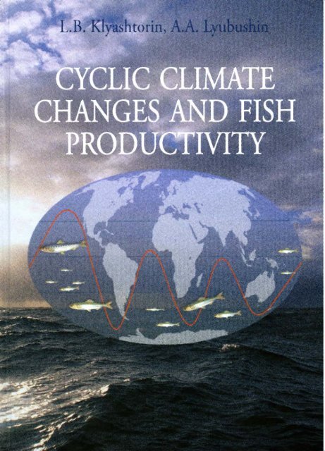
GOVERNMENT OF THE RUSSIAN FEDERATIONSTATE COMMITTEE FOR FISHERIES OF THE RUSSIAN FEDERATIONFEDERAL STATE UNITARY ENTERPRISE«RUSSIAN FEDERAL RESEARCH INSTITUTE OF FISHERIESAND OCEANOGRAPHY »(FSUE «VNIRO»)L.B. KLYASHTORIN, A.A. LYUBUSHINCYCLIC CLIMATE CHANGESANDFISH PRODUCTIVITYEDITOR OF ENGLISH VERSION OF THE BOOKDR. GARY D. SHARPCENTER FOR CLIMATE / OCEAN RESOURCES STUDYSALINAS, CALIFORNIA, USAMoscow VNIRO PUBLISHING 2007

УДК 639.2.053.8:551.465.7:639.2.053.1KLYASHTORIN L.B., LYUBUSHIN A.A.K47CYCLIC CLIMATE CHANGES AND FISH PRODUCTIVITY.— M.: VNIRO PUBLI­SHING, 2007.— 224 P.The book considers relationships between climate changes and fish productivityof oceanic ecosystems. Long-term time series of various climatic indices, dynamicsof phyto- and zooplankton and variation of commercial fish populations in the mostproductive oceanic areas are analyzed. Comparison of climate index fluctuations andpopulations of major commercial species for the last 1500 years indicates on a coherentcharacter of climate fluctuations and fish production dynamics. A simple stochasticmodel is suggested that makes it possible to predict trends of basic climaticindices and populations of some commercial fish species for several decades ahead.The approach based on the cyclic character of both climate and marine biota changesmakes it possible to improve harvesting of commercial fish stocks depending on aphase (ascending or descending) of the long-term cycle of the fish population. Inaddition, this approach is helpful for making decisions on long-term investments infishing fleet, enterprises, installations, etc. The results obtained also elucidate the olddiscussion: which factor is more influential on the long-term fluctuations of majorcommercial stocks, climate or commercial fisheries?ISBN 978-5-85382-339-6© Klyashtorin L.B., Lyubushin A.A., 2007© VNIRO Publishing, 2007

INTRODUCTIONMANY CENTURY-LONG FISHERY PRACTICES INDICATED THAT THE POPULATIONS ANDCATCHES OF MASSIVE COMMERCIAL FISHES, HERRINGS, CODFISH, SARDINES, ANCHOVIES,SALMONS AND SOME OTHER SPECIES ARE SUBJECT TO SIGNIFICANT LONG-TERM FLUCTUA­TIONS [ROTHSCHILD, 1986; SHARP, 2003].THE PERIODS OF «GOOD» OR «POOR» FISHERIES HAVE CAUSED AND STILL CAUSESIGNIFICANT ECONOMIC AND SOCIAL CONSEQUENCES. AS INDICATED IN JAPANESEANNALS, OUTBURSTS IN POPULATION AND CATCHES OF JAPANESE SARDINE ATTRACTED PEO­PLE TO THE SEA AND CAUSED EXPANSION OF SEABOARD INDUSTRIAL FISHING SETTLE­MENTS, WHEREAS DIMINUTION OF THE FISHED POPULATIONS AND CATCHES CAUSEDWITHDRAWAL OF THE PEOPLE, AND SOME SETTLEMENTS DISAPPEARED. WITHIN THE RE­CENT 400 YEARS THIS PROCESS REPEATED EVERY 50 TO 70 YEARS [KAWASAKI, 1994].THE WRITTEN HISTORY OF RISES AND FALLS OF BOHUSLAN HERRING CATCHES AT THESOUTHERN EXTREMITY OF SWEDEN IN THE SKAGERRAK STRAIT EMBRACES OVER A THOU­SAND YEARS. THE FIRST DOCUMENTED ATTEMPTS TO DETECT THE PERIODICITY OF THISPROCESS WERE INITIATED IN THE 19 T HCENTURY [LJUINGMAN, 1880]. THE AVERAGEDURATION OF «GOOD» OR «POOR» PERIODS HAS BEEN SHOWN TO BE ABOUT 55 YEARS,AND THE FULL FLUCTUATION CYCLE FOR THE BOHUSLAN HERRING BLOOM / BUST PATTERN IS110 TO 120 YEARS. THIS REPEATING PATTERN HAS TENDED TO ASSOCIATE WITH SECULARALTERATION OF THE SOLAR ACTIVITY (SUN SPOT DYNAMICS) AND POLAR LIGHTS (GALACTIC-RAYS). MODERN RESEARCHERS SUGGEST THAT THE PERIODICITY OF BOHUSLAN FISHERYRELATES TO LONG-PERIOD METEOROLOGICAL PROCESSES PROCEEDING IN NORTH ATLANTICAND SPECIFICITY OF HERRING MIGRATION IN THE NORTH SEA AS A RESPONSE TO THECHANGES IN OCEANOGRAPHIC CONTEXTS [ALHEIT, HAGEN, 1997; CORTEN, 1999].DURING THE LAST CENTURY, SYNCHRONOUS OUTBURSTS IN PACIFIC SARDINE POPULA­TIONS (JAPANESE SARDINE Sardinops melanostictus), CALIFORNIA AND PERUVIAN3

Sardinops sagax) were observed with approximate 60-year period thusinducing rise and fall of the extensive Japanese seaboards' regional economicevolution. Dramatic fluctuations of the Peruvian anchovy populationinduce significant changes in fish-meal production, one of the basic exportproducts of Peru. Similarly, fluctuations in the reserves of Northern Pacificpollack, observed during the recent 50 years, were followed by seriouschanges in «surimi» (imitation crabmeat) production, which provides sufficienteconomic incentives for the fishing industries of several countries.Already in the 1950s, concepts about relationships between climateprocesses and fluctuations in the population of commercial fishes were formulatedby G.K. Izhevsky [1961; 1964]. He related fluctuations in the populationsand hauls of Atlantic cod, herring and some other commercial fishesto multiyear eurhythmies of the solunar tidal forcing, variations in North-Atlantic Drift intensity, fluctuations in the heat delivery to the Arctic region,and the temperature variation in the 0-200 meter layer in the «Kola Meridian*.In the recent fifty years an immense extent of new data was obtained,and understanding of the mechanisms of oceanic and climatic processes becamemore profound, hence Izhevsky's ideas are still useful [Elizarov, 2001].In her famous monograph, T.F. Dementieva developed the ideas aboutdependence of long-period fluctuations of commercial fish population onclimate changes [Dementieva, 1976].The problem of climate change influences on the North Pacific fishcapacity was considered in a series of works by V.P. Shuntov et al. [Shuntov.VasiTkov. 1982; Shuntov, 1986, 1991, 2001]. Cushing [Cushing, 1982]and Laevastu [Laevastu, 1993] each wrote monographs devoted to findinga relationship between climate and fishery which each exerted a significanteffect on the formation of ideas describing the reasons of fluctuations in thepopulation of some commercial fishes, although the greater part of theirresults were derived from the data from only the North Atlantic. Since thesereports were published, interests in global studies of the Earth climate havegrown significantly and thus the volume of climatological data has also dramaticallyincreased, while the geography of fishery zones were extended,and commercial catch statistics sequences have expanded.The works by Lluch-Belda et al., Kawasaki and some other researchers[Lluch-Belda et al., 1989; 1992a, b; Kawasaki, 1992a, b; 1994; Schwartzloseet al., 1999], devoted to searching for the reasons of synchronous alterationsof sardine and anchovy population increases in different regions, haveattracted attention to the problem of possible existence of a global «climatic4

signal» which synchronizes changes in ecosystems of different regions of theWorld Ocean.Recently, 60-70 year repeating alterations of hemispherical and globalclimate were detected [Schlesinger, Ramankutty, 1994; Minobe, 1997,1999,2000]. Temperature sequences for the recent 1500 years, reconstructed fromGreenland ice core samples, show domination of approximately 60-yearperiodicity of the climate fluctuations [Klyashtorin, Lyubushin, 2003; Klyashtorin,Lyubushin, 2005]. For the same period, similar (50-70 year) temperatureperiodicity was detected in the analysis of long-living tree annualgrowth rings in the Arctic region and California. Reconstruction of sardineand anchovy population fluctuations by analysis of scales in bottom sedimentsin Californian upwelling for the latest 1700 years has indicated theirapproximately 60-year periodicity [Baumgartner et al., 1992].The role of climate as the main factor defining fluctuations in the populationsof Pacific salmon and some other commercial species is shown in aset of recent works [Birman, 1985; Beamish, Bouillon, 1993; Jonsson, 1994;Klyashtorin, Smirnov, 1995; Klyashtorin, Sidorenkov, 1996; Klyashtorin,2001; Chavez et al., 2003].The main topic of this book is studying a relationship between cyclic e.g.more or less regularly repeating long-period climate changes and fish capacity/ distribution and abundance changes. This requires demonstration of arelationship between repeating changes in the climate and fish capacity / distributionand abundance changes, as well as finding approaches to develop amodel that successfully predicts possible fluctuations in the reserves of themain commercial species over the perspective of several decades.Populations of the main commercial fish species that yield up to 40% ofthe world total fish landings are subject to long-period fluctuations inducingvarious fishery and economic events. More or less reliable relationshipsbetween climate variations and the fish capacity may be set using multiyearsequences of the population fluctuations of the largest commercial populationswith annual landings that have reached over a million tons.Time scale of the climate changes is two-three decades, and the spatialscale is several million square kilometers. There is to date no unified theoryof the climate system of the Earth, and many climatological aspects are notalso well elucidated. It is thus not our goal to discuss particular mechanismsof the climatic processes. In order to characterize long-period changes in theclimate the results of intensive climatologic studies have been used, the socalled«climatic indices» with dynamics that show climate changes for many5

decades, either global, hemispherical or regional. Our focus is on the practicaland important question of the relationships between climate changes andthe resulting productivity of oceanic ecosystems. Comparative data on therate of climatic indices, dynamics of phyto- and zooplankton and commercialfishery populations in the productive zones of the ocean are considered.Analysis of the data on fluctuations of the climate and populations of somemassive commercial fisheries during the latest 1500 years allows realisticconjugation of the climate and fisheries capacity fluctuations. Based on theresults obtained, we provide a stochastic prognostic model of the fluctuationsof climate and population for several of these large populations of commercialspecies for the prospect of several decades. The ideas about cyclic characterof the climate and biota fluctuations allow modification of commercialoperations, as we have described, and at which phase of the long-periodcycle (fall or rise of the population) each of these commercial fisheries populationsis in now, or will experience. This approach promotes feasibleinvestments into long-term projections of commercial fleet or fish-processingenterprise management.The results obtained clear up an old question under discussion about thereason for the long-period fluctuations of the resources of the main commercialspecies: climate or the large-scale fishery.Note: Abbreviations are shown at the end of the book.6

CHAPTER 1ON CLIMATE REPEATING PATTERNThe term «climate» is defined as long-term statistically averaged weatherindices. To smooth inevitable seasonal and annual variations, the averagingperiod should amount to decades. International meteorological conferencesheld in 1935 in Warsaw and in 1957 in Washington to determine characteristicsof the modern climate recommended 30-year averaging periods[Monin, Shishkov, 2000].Spatial parameter is the second important index for the climate estimation.To obtain statistically reliable climatic characteristics the Earth surfacearea used for the long-term analysis should be rather large. As shownby A.V. Kislov et al. [2000], the minimum area for data collection equals1-3 mill. km 2 .Thus, the time scale of climate changes equals several decades and thespatial scale gives several million square kilometers. In actual practice, climaticvariability is usually described by 10-30-year averaging for aquaticareas of million square kilometers.SHORT-PERIOD TIME SERIESRegular and reliable instrumental measurements of the surface layer airtemperature were initiated about 150 years ago. The average temperatureanomaly of the surface air layer (Global dT), averaged by all measurementpoints, is considered to be the most important index characterizing globallong-period fluctuations of the Earths climate [Bell et al., 2001; Jones et al.,7

2001]. It is this index considered to be the main characteristic of dynamicsof the so-called global warming.Fig. 1.1 shows dynamics of Global dT for the 140-year observation periodand its annual fluctuations. Inter-year variations are rather large andshould be smoothed in order to detect long-period behavior of Global dTfluctuations. For this purpose, a 13-year moving averaging is usedFig. 1.1. Dynamics of the surface air Global temperature anomaly (Global dT)1861-2000. Dotted line shows annual variations of Global dT, bold line is the samesmoothed by 13-year moving averagingAs shown in Fig. 1.1, the increasing secular linear trend (about 0.06 °Cper each 10 years; Sonechkin, 1998) at the background of interannual yearGlobal dT variations is observed.At the background of the secular linear trend, Global dT undergoes longperiod,up to 60-year long, fluctuations. These fluctuations can be detectedby detrending with the help of a standard statistical operation [Statgraphics,1988]. After detrending, the long-period fluctuations of Global dT with themaxima at about 1870s, 1930s and, apparently, at 1990s are clearly observed(Fig. 1.2). Global dT detrending allows detection of 2.5 cycles of approximately60-year Global dT fluctuations.8

Fig. 1.2. Dynamics of detrended Global dT, smoothed by 13-years moving averagingAn approximately 60-year repeating pattern is also observed well fromtemperature anomaly dynamics in the circumpolar Arctic zone (Arctic dT)between 60 and 85° N. Detrended Global dT behavior compared with ArcticdT is shown in Fig. 1.3.Fig. 1.3. Comparative dynamics of detrended Global dT (bold line) and temperatureanomaly of Arctic circumpolar zone (Arctic dT). 60-85° N, (white squares)13-year smoothing. Data from Alexandrov et al., 20039

happen, with type E processes, when such processes are disturbed or changedto the opposite ones. On the other hand, due to strict geographical localizationof C circulation (from north to south and from south to north — L.K.) they cannotbe mixed with the circulation types W and E».Each of the above-mentioned forms is determined by analyzing dailyatmospheric pressure maps for Atlantic-Eurasian region. The direction of cyclonicand anticyclonic air mass transfers is elucidated by distribution ofatmospheric pressure fields based on analysis of the general picture of the«atmospheric pressure topography» in the region.However, there is some «asymmetry» in the Vangenheim-Girs system.If types E and W each marks an individual direction of the atmospherictransfer to the east or to the west, type C unites «meridional» transfers inthe north (N) and south (S) directions and represents their sum (N + S). Byanalogy, an association of atmospheric transfers of east (E) and west (W)directions into one «zonal» type (W + E) is suggested.Recurrence of meridional (N + S) and zonal (W + E) transfer are transformedas anomalies (deviation of the repetition of each shape from thelong-term average). The sum of anomalies of all types per year equals zero:(N + S) + (W + E) = 0 and (N + S) = (W + E).Thus far, for each transform 110 mean-year anomalies of their repetitionsare accumulated. For characterization of long-period changes in circulationwe use not a sequence of anomalies themselves, but the so-called «integralcurve», obtained by sequenced summation of anomalies that represents a curveof accumulated frequencies (cumulative curve).This index called Atmospheric Circulation Index (ACI) characterizesthe long-period dynamics of zonal and longitudinal transfer processes inAtlantic-Eurasian region. Fig. 1.4 shows zonal and longitudinal ACI patternfor the latest 110 years.As shown in Fig. 1.4, zonal and meridional ACI curves are antiphase,have no secular linear trend, and their fluctuations have approximately60-year period. ACI dynamics characterizes the long-period behavior ofatmospheric processes in North Atlantic. First of all, they should be comparedwith Arctic dT dynamics that reflect temperature variations in the latitudinalzone of 60-80° N. Fig. 1.5 shows full coincidence of Arctic dT andzonal ACI dynamics.The comparison of zonal ACI and Global dT behaviors (Fig. 1.6) demonstratestheir close affinity, although ACI curve precedes Global dT changes11

y approximately 5 years. Thus, zonal ACI, the index regional by origin, maybe considered as a climate index, which similar to Global dT reflects globalchanges in climate of the Earth.Fig. 1.4. Dynamics of zonal (bold line) and meridional (thin line) AtmosphericCirculation Index (ACI), 1891-2000. The data were kindly provided by Dr. V.V. Ivanovfrom Arcticand Antarctic Research Institute (AARI), St.-Petersburg12Fig. 1.5. Comparative dynamics of zonal ACI (bold line) and Arctic dT (whitesquares), smoothed by 13-year averaging, 1891-2000

YearsFig. 1.6. Comparative dynamics of detrended Global dT (bold line) and zonal ACI(thin line), 1861-2000In accordance with Global dT, zonal ACI increases in the periods of«warming», whereas decreases in the periods of «cooling». The comparisonof zonal and longitudinal ACI fluctuation dynamics (see Fig. 1.4) showsthat the dominance periods of each of these shift sign approximately every30 years. These periods, called «zonal» and «meridional» climatic epochs,coincide with the periods of warm and cold epochs according to the longperioddynamics of Global dT fluctuations (see Figs. 1.5 and 1.6).For separating climatic epochs by alteration of atmospheric circulationforms (see Fig. 1.4) and Global dT fluctuations (Fig. 1.6) only upper partsof the curves are used. The scheme in Fig. 1.7 clearly demonstrates alterationof warm (zonal) and cold (meridional) epochs with approximately 30-yearrepetition during the last 110 years. On this basis it is reasonable that the currentwarm or zonal climatic epoch, started in 1970s, will probably finish inthe first decade of 2000s, and the subsequent cold epoch will last since 2010still 2030s (Fig. 1.7).The above-considered climatic indices were mainly obtained fromobservations in Atlantic region. In Pacific region two climate indices arewidely used: Pacific Decadal Oscillation (PDO) and Aleutian Low PressureIndex (ALPI).PDO characterizes the long-period temperature changes of Pacific Oceansurface in its northern part [Barnett et al., 1999; Hare, Mantua, 2000].13

Fig. 1.7. Alteration of the warm (bold line) and cold (thin line) climatic epochsby fluctuations of the Global temperature anomaly (Global dT) and AtmosphericCirculation Index (ACI). Dashed thin line shows probable transfers intothe next cold epochALPI characterizes the long-period changes in the area of low atmosphericpressure in North Pacific (mill. km 2 ). It is considered as one of themain climate indices for this region [Beamish, Bouillon, 1993; Hare,Mantua, 2000].Beside ALPI, the North Pacific Index (NPI) is also used, which characterizesthe long-period changes of the atmospheric pressure in the entirewater surface area of North Pacific [Trenberth, Hurell, 1995]. Dynamics ofthis index represents a mirror reflection of ALPI [Hare, Mantua, 2000].Fig. 1.8 shows comparison of Atlantic, Pacific and global climatic indicesbehavior for the last 100 years. It is clear that PDO and ALPI dynamics isclose to that of detrended Global dT, as well as to Arctic dT and zonal ACI.All curves have clear periods of both minima (1900s-1920s and1960s-197()s) and maxima (1930s-1940s and 1980s-1990s). Note also thatPDO and ALPI (as well as Arctic dT) virtually have not rising trend.Moreover, regional Pacific PDO and ALPI indices have definite differencesfrom Global and Arctic dT. A maximum in the mid 1980s and an intermediateminimum in the mid 1990s are typical of PDO and ALPI, whereas in themiddle 1990s Global dT and ACI curves each show the beginning of a maximum.Both global and regional climatic indices demonstrate general cyclicdynamics with approximately 60-year period.14

Resemblance of the long-period dynamics of these main climatic indicesindicates existence of a «global climatic signal» e.g. simultaneous developmentof climatic processes having approximately 60-year periodicity,observed, at least, for the whole northern hemisphere.YearsFig. 1.8. Comparative dynamics of several climatic indices for 1900-2000:Pacific Decadal Oscillation (PDO), Aleutian Atmospheric Presssure Index (ALPI),zonal ACI, detrended Global dT and Arctic Temperature Anomaly (Arctic dT).Smoothed by 13-year moving averaging15

The basic results indicate an approximately 60-year periodicity of climaticprocesses. These results are based on the analysis of relatively shortobservation periods, generally about 100 years, and the only longer empiricalobservation time series is that for Global dT, which comprise 140 years.Reliable detection of climatic processes requires analysis of much longerclimatic data series, as long as several hundred or even thousands of years.Such time series were obtained by reconstruction of paleotemperaturefrom isotopic analysis of large glacier columns or analysis of annual growthrings of long-living trees.LONG-TERM CLIMATIC TIME SERIESFig. 1.9 shows time series for temperature over the last 1500 years,reconstructed by the analysis of Greenland ice core samples and annualgrowth rings of the long-living trees: Arctic pine tree from ScandinavianPeninsula and North-California bristlecone pine tree.After smoothing these annual temperature variations by 41-year movingaveraging, multidecadal temperature fluctuation periodicity is detected withthe help of spectral analysis methods.Temperature fluctuations reconstructed byin the Greenland ice cores1 80Polar glaciers contain paleoclimatic information in the form of heavyoxygen isotope, 1 8 0, content in the ice [Dansgaard et al., 1975]. Isotope 1 8 0concentration is measured in parts per million in relation to its content in theso-called «standard oceanic water». As the air temperature increases, the relativenumber of water molecules with increased content of heavy oxygenisotope rises as their rate of evaporation from the ocean surface increases.Water vapors are transferred poleward by air flows to the North, and aftertheir condensation above Greenland, the snow formed is gradually transformedto ice. Variations in 1 8 0 content along the borehole in ice show airtemperature fluctuations in the region at the moment of snowfall to ancientglacier surfaces.In the central part of Greenland (at about 71° N) the conditions of snowaccumulation and ice formation remained stable during several thousand16

Fig. 1.9. Reconstructed temperature and humidity time series for 1500 years. Thinlines show annual data, bold lines give 41-year moving averaging by: a — Greenlandice cores, b — Arctic pine tree rings, c — California pine tree rings17

years. «Nowhere else in the world is it possible to find a better combinationof a reasonably high accumulation rate, simple ice flow patterns (which facilitatesthe calculation of the time scale), high ice thickness (which offers adetailed record, even at great depths) and meteorologically significant location(close to the main track of North Atlantic cyclones». [Dansgaard et. al.,1975]. Analysis of l s O content in the ice core of more than 500 m in depth(with annual section thickness of 0.29 m) made it possible to reconstruct themean annual air surface temperature for last 1423 years (from 552 to 1975).Fig. 1.10 shows the full spectrum of temperature fluctuations fromGreenland Ice core samples over almost 1500 years.Of the greatest interest are fluctuations with «climatic» periodicities of20 to 100 years. As the graphic shows, 19 and 54 year periodicities are mostclearly expressed; the 160-year cycle is also clear.18Fig. 1.10. Spectrum of periodical temperature fluctuations for 1423 years byGreenland ice core samples (logarithmic X-axis). Ordinate — spectral power.Abscissa — period, years

Temperature fluctuations for 1400 years(from 500 thto 1900 th ) reconstructed by annual growthrings of pine tree (Pinus silvestris) in the North of SwedenIn Arctic regions trees grow in warm seasons only. This fact makes annualgrowth rings clear enough for reliable reconstruction of summer temperature.One of the most reliable long-period reconstructions was performedon growth rings of long-living pine tree from the North of Sweden[about 68° N; Briffa et al., 1990]. The full spectrum of temperature fluctuationsis shown in Fig. 1.11.Fig. 1.11 shows that 16.8-, 32-, 60- and 108-year periodicity are predominant.According to growth rings of Norway pine from Lofoten Islands,analysis of temperature fluctuations for the last 300 years yielded quite similarpredominant periodicities: 17.5, 23 and 57 years [Ording, 1941; Ottestad,Fig. 1.11. Spectrum of periodical temperature fluctuations for 1400 years by theArctic pine tree (Pinus silvestris) growth rings (logarithmic X-axis). Ordinate —spectral power. Abscissa— period, years19

1942]. The periodicities most interesting for us are those of 57 and 60 years,which are very close from estimations of different authors.Moisture / Aridity fluctuations for 1480 years(500 th to 1980 th ) reconstructed by growth ringsof North California bristlecone pine tree (Pinus aristata)One of the longest climatic time series is the dendrochronology series(growth rings) changes for the oldest trees, the bristlecone pine, that grows atabout 3000 meters above sea-level in the North Californian western ridgesof the Great Basin. This year-ring series is almost 8000 years long (from6000 A.C. until 1979 A.D.) that is called the Methuselah Walk Pilo (D. Graybill).The spectrum of final part (1500 years) of time series shown in20Fig. 1.12. Spectrum of periodical moisture fluctuations for 1500 years according toCalifornia bristlecone pine (Pinus aristata) tree growth rings (logarithmic X-axis).Ordinate — spectral intensity

Fig. 1.12 (http://www-personal.buseco. monash.edu.au/~hyndman/TSDL/ aswell as http://www.ncdc.noaa. gov/paleo/treering.html).Variations of the pine tree growth ring thickness depend on moisture contentfluctuations reflecting droughts strength in the south of the North-American continent and, obliquely, fluctuations of the surface temperature ofthe entire Northern hemisphere. This known time series is the subject fordetailed study, and its dynamics is similar to the 1500-year dendrochronologyseries of the North Scandinavian pine (Pinus sylvestris L.) tree and withthe 10000-year series of bottom sediments from Lake Tingstede [Monin,Sonechkin, 2005].ANALYSIS OF LONG-PERIOD TIME SERIES SPECTRASpectral analysis is used for detecting the most frequently repeating (predominant)periodical fluctuations of any index, for example, temperature orfish population abundance.Relatively «high-frequency» regions of the spectra reflecting temperaturefluctuations shorter than 20 years are not sufficient for detecting processesof «climatic» duration. Of the greatest interest for our ecologicallysignificant estimation of climatic processes periodicity is the range of 20 to100 years. Fig. 1.13 shows curves of predominant periodicities in the rangeof 20 to 100 years.The spectrum of Greenland ice core samples (Fig. 1.13,a) shows predominanceof a 54-year periodicity, the 32-year peak is less intensive. Spectrumof Arctic pine tree shows predominance of the 60-year peak, whereasthe 32-year peak is lower (Fig. 1.13,/?). The spectrum of California bristleconepine (Fig. 1.13,c) shows predominance of the 76-year peak, whereas26- and 39-year peaks are less intensive. These are somewhat longer than theperiodicities obtained for ice core samples and Arctic pine tree. At the sametime, the full time series of California bristelcone pine tree growth rings isabout 8000 years, and that gives a possibility to track changes in periodicityof temperature fluctuations. Results of the spectral analysis of the entire8000-year series shows predominance of the 55.4-year peak (Fig. 1.13,J).This spectral peak corresponds to predominant peaks (54 years) in the spectrumof ice core samples and is close to the 60-year periodicity for the spectrumof Arctic pine tree growth rings (Fig. 1.13,6).21

Fig. 1.13. Spectral density of the climatic periodicity maxima over the time rangeof 20-100 years: a — Greenland ice core samples, b — Arctic pine tree growthrings, c — California bristlecone pine tree growth rings, d — California bristleconepine tree growth rings for the last 8000 years (logarithmic X-axis)Fluctuations in populations of sardine and anchovyaccording to the data of fish scales analysis in bottomsediment layers of California upwellingIn recent decades data have been gathered that allow observation of fluctuationsin sardines and anchovy populations during the recent 2000 yearsthe in California coastal upwelling zone.22

In anoxic basins of Pacific Ocean seabeds, particularly in the region ofSouthern California Bight upwelling, region fish scales residues are accumulatedfrom the most abundant species, sardine (Sardinops caeruled) andanchovy (Engraulis mordax), observed in this region. No decomposition oforganic residues (fish scales, in particular) happens due to stable anaerobicmode in these sediment basins.Bottom sediment bore samples from this region demonstrate clear layeredstructure many meters deep. The lamina-based analysis of sardine andanchovy scales in the samples of sediments allowed reconstruction of populationfluctuations for these species for 1700 years [Baumgartner et al.,1992]. Dynamics of reconstructed fluctuations of sardine and anchovy biomassesfrom this work are shown in Fig. 1.14.Fig. 1.14. Biomass fluctuations of (

Fig. 1.14 shows that within the 1700-year series the populations of bothspecies fluctuated significantly: outbursts of the populations were followedby changes with periods of their almost complete disappearance. These fluctuationshappened exclusively under the effect of natural (climatic) factors,i.e., without any effect of any fishery. Typically, modern fluctuations of sardineand anchovy populations in the 20 thcentury, when they were intensivelyfished , demonstrated practically the same periods and amplitudes comparedwith the natural fluctuations during the last 2000 years [Baumgartneret al., 1992].Fluctuation spectra of California sardine and anchovy populations duringthe recent 1700 years (Fig. 1.15) demonstrate well defined predominantpeaks: 57 and 76 years for sardine and 57, 72, and 99 year for anchovy. Thiscorrelates well with the predominant spectra of climatic fluctuations duringthe last 1500 years according to ice core samples and tree growth rings.Period, yearsPeriod, yearsFig. 1.15. Periodicity spectra of biomass fluctuation for (a) California sardine(Sardinops cearulea) and (b) anchovy (Engraulis mordax) reconstructed by thefish scale deposition in the sediment cores. Data from Baumgartner et al., 1992,slightly modifiedAnalysis of reconstructed and experimental spectraTo compare with the results of long time series analysis, the data of spectralanalysis of relatively short series of Global dT from instrumental measurementsand Atmospheric Circulation Index (ACI) (Vangenheim-Girs referencehere!) with the predominant periodicity of 55 and 50 years, respectively,are shown in Fig. 1.16.Table 1 presents general distribution of predominant periodicities of theabove-considered time series.24

Data in the Table shows that predominant periodicities for climatic andfish populations series correlate well, falling within the range of 54 to 76 yearswith the general average of 59.2 years. Data for California bristlecone pineFig. 1.16. Time series spectra of Global dT (a) for 140 years (instrumental measurements)and Atmospheric Circulation Index (ACI) (b) for 110 years (logarithmicX-axis, years)Table 1. Predominant periods of climatic fluctuations within the range of 20-100 years according to all data availableTime seriesSeries length,yearsPredominantpeak, yearsSecondarymaxima, yearsIce core samples 1420 (552-1973) 54 32Arctic pine tree 1480 (500-1980) 60 32California bristleconepine tree 1500 (479-1979) 76 32California bristleconepine tree 8000 (-6000-1979) 55.4 20-35Sardine (sediment coresamples) 1730(270-1970) 57 and 76 56. 33Anchovy (sediment coresamples) 1730 (270-1970) 57 72, 99Global dT 140(1861-2001) 55 18.0Atmospheric CirculationIndex (ACI) 110(1891-2001) 50 19.025

tree are slightly different from the general average, although a 55-year periodicityis definietely detected at the analysis of the 8000-year time series.The most reliable data on long-period dynamics of the mean annualtemperature are given by analysis of isotope 1 8 0 content in Greenland icecore samples. Results shown in the Table show that for the last 1500 yearsthe predominant periodicities of climate and biota fluctuations were aroundthe 60-year average. Higher frequency (13-23 year) fluctuations are also ofinterest, however, reliable relationships between them and broad scale fishpopulations fluctuations cannot be detected.The data obtained characterize the periodicity spectrum for each entire1500-year series. However, understanding of the long-period climate fluctuationsrequires the knowledge how these predominant periodicities are distributedin time for the last millennia. These data may be obtained with thehelp Time-Frequency spectral Analysis (TFA).TIME-FREQUENCY SPECTRAL ANALYSISOF LONG-PERIOD CLIMATIC SERIESFig. 1.17 (see tinted insert) shows 3D relief diagrams of common logarithmdevelopment for intensities of the three long-term climatic time series.They are composed as follows. The time window of 600 counts (600 years)is shifted along the time series from the left to the right with 50-year time steps;for each location of the time window an intensity spectrum for the time seriesfragment, that occurred in each window, was estimated. The estimation wasperformed by the maximal entropy method with autoregression order 60.Thus, a dependence of the intensity spectrum estimation on two parameterswas obtained: the frequency, as usual, and the time window location. Thisdependence may be visualized shaped as a 3D «mountain relief», where theordinate is frequency and the abscissa is the right end of the time windowlocation, and «by height» the common logarithm of the intensity spectrum ismeasured. The data are visualized by popular graphic software Surfer.Diagrams of this type allow illustration of time-dependence of a selectionof climatic series periodicities, shaped as 3D color pictures resembling landscapesof mountain chains aligned along the time scale (by abscissa). Theheight of «ridges» is defined by manifestation intensity e.g. by frequency ofthis periodicity, in accordance with the scale of periods (by the ordinate).26

Moreover, the intensity of periodicity occurrence is demonstrated by colors:low intensity is blue through green to yellow, and high is from orange tored. White «peak tops» mark the highest frequency of this periodicity, forinstance, 18.5-year periodicity (Fig. 1.17,a) or a maximum of 60-70-yearperiodicity (Fig. 1.17,6) at the end of the 20 thcentury.Tracking the height of «ridges» with time in Fig. 1.17, one may imaginehow the intensity of one or another periodicity has been changing during thelast 1000 years. The use of 3D diagrams provides a clear view that climaticfluctuations are cyclic, but the intensity of climatic cycles undergo significantchanges with time.Fig. 1.17,a shows, how the intensity of periodical temperature fluctuations(change their periodicity) with time from analysis of Greenland icecore samples. It is clearly observed that maxima of cyclic temperature fluctuationsare distributed irregularly in time. The periodicity of 160 years iswell expressed from the early 1200s until the late 1300s, and then disappeared.The 33-year periodicity is observed only between 1300s and 1700s,and then practically disappears, too. On the contrary, intensity of the 55-yearperiodicity continuously increased from 1500s and reached the maximum atthe late 1990s.Fig. 1.17,6 shows time dynamics of the temperature periodicity, determinedby the growth rings of Arctic pine tree from the North Sweden. It isclear that in the recent millennium 60-70 years was the predominant periodicityof temperature fluctuations. Its intensity was not so high in the periodof 1750s until 1800s, but increased by the end of 1900s.Fig. 1.17,c illustrates temporal dynamics of moisture/aridty fluctuationsfor California bristlecone pine tree data. Intensity of the mostly expressedperiodicity of 65-75 years gradually increased from 1100s to their maximumat 1600s and is preserved at the level until the end of 1900s. The 25-27-yearperiodicity is observed only since the middle 1500s, and then its intensitygradually increased by the end of the 20 thcentury. Periodicities of 18.5 and12.5 years are detected only in the recent 300 years.Note also that the data on the growth rings of trees characterize only summermoisture and related temperatures. The most reliable data on the meanannualtemperature are given by the analysis of heavy isotope ls O content inGreenland ice core samples.As observed from the plots, 55-70-year periodicity is expressed muchmore strongly relative to other periodicities. Hence, 55-70-year and othertemperature periodicities are distributed irregularly in time for the entire27

This proper classification of climatic time series behavior may relate tothe existence of time intervals with low and high predictability of the climate,see Chapter 7 for details. Here we specifically want to note that theexistence of strong monochromatic components in the signal variationsallows sharp increase of both efficiency and «hitting range» of the time seriesprediction due to the use of cyclical trends with the period of that monochromaticcomponent (periodicity), which is predominant in the currentperiod of time. If there were no predominant monochromatic components,this scheme of prediction is not valid, so we would then have to cope byusing the usual prediction methods basied on correlations of neighboringvalues in the time series, which may be effective for 1-2 steps only e.g. thepossibility of long-term prediction simply disappear.In the context of such separation of the climate history into intervals of lowand high predictability, it is of interest to overlook the evolution of intensityspectrum in the low-frequency range. The 8000-year time series of Californiabristlecone pine tree growth rings provides an opportunity to consider thechange of intensity in the long-term climatic periodicities within a longertime period.We have analyzed variability of the intensity spectrum for Californiabristlecone pine tree growth rings for 8000 years in the periodicity range of40 to 200 years in a sliding time window 600 years long. For each locationof this time window in the selected range a maximum of intensity spectrumlogarithm was detected. The results are shown in Figs. 1.18 .As observed from Fig. 1.18 plots, periodicity of low-frequency cyclesvaries significantly with time in the periods of 2000 to 1500 years. At theminimal level, periodicity of these cycles is sustained during 500-1000 yearsuntil the next period of growth, whereas at the maximal level it is maintainedfor only 200-500 years. Maxima on the curve correspond to time intervals ofhigh potential predictability, and minima correspond to the periods of lowpredictability. However, this predictability is just potential; to make it real,we must make sure that the maximum value on this plot corresponds tooccurrence of a signal localized by frequency (narrow band) rather than tosteady increase of the intensity spectrum in the entire low-frequency range.In this case, prediction using a local cyclic trend can be applied.For more accurate assessment of values of this increasing periodicity onehas refer to TFA plots in Fig. 1.17. As all the plots clearly show, for the last1000 years the periodicity of 50-70 years was predominant, and its recur-30

Fig. 1.18. Intensity spectrum variation for temperature (humidity/aridity) fluctuations,obtained from California bristlecone pine tree growth rings, in the frequencyrange of 0.025 to 0.005 year 1(40-200 years) in the moving 600-yeartime window. Y-axis is intensity spectrum logarithm; X-axis is years at rightend of the time windowrence steadily increased. As a consequence, for the long-period prediction ofthe climate fluctuations (for several decades ahead) it is reasonable to use theestimate of this cyclic trend (see Chapters 7 and 8).Thus, by the end of the 20 thcentury recurrence of the 50-70-year periodicityreached its regular maximum and will likely be sustained at this level,at least over the following century. This increases the reliability of perspectiveforecasts of long-period climate and biota dynamics.Climate periodicity of about 50-70 years has been detected by variousauthors. Spectral analysis of temperature variability series in North Americaand Europe for the last 1000 years indicated predominance of cyclic temperaturefluctuations within the range of 60 to 80 years and at 120 years[Shabalova, Weber, 1999]. In the work by Schlesinger and Ramankutty[Schlesinger, Ramankutty, 1994] predominance of 65-70-year periodicity ofthe global climate was demonstrated. Spectral analysis of the long-perioddynamics of the ocean surface temperature and atmospheric pressure inNorth Pacific water area [Minobe, 1997, 1999, 2000] during the last centurydemonstrated predominant 50-70-year (and additional 20-30-year) periodicityof climatic indices PDO and ALPI. Similar data on the 50-70-yearperiodicity of ocean surface temperature fluctuations (PDO index) wereobtained by Mantua and Hare [Mantua, Hare, 2002].31

Comments in briefAnalysis of the three 1500-year long time series of reconstructed temperatures(and humidity/aridity) (Greenland, Scandinavia, California) indicatethe predominant periodicity of climatic fluctuations during the last1000 years equal about 60 years with the variation from 55 to 76 years.The second intensity spectral peak of periodicity occurs at 30-32 years. Theexistence of these climatic periodicities (50-70 and 30 years) is confirmedin by several authors [Schlesinger, Ramankutty, 1994; Minobe, 1997, 1999,2000].Temperature reconstruction by analyzing Greenland ice core samplesfor the last 1400 years characterize winter temperature, which practicallydetermines fluctuations of the mean annual temperature. The predominant55-year periodicity of the mean annual temperature detected by ice coresamples is similar to periodicities of Global dT and ACI, instrumentallymeasured during the last 140 and 110 years, respectively.For the last 1700 years, fluctuation periodicities of Californian sardineand anchovy populations approach climatic fluctuations falling within therange of 55-75 years. The intensity of 50-70-year periodicity have continuouslyincreased during the last millenia and reached its maximum in the endof the 20 thcentury. Basing on the increasing dynamics of the 55-70-yearperiodicity intensity for the last 1000 years, it may be suggested that thisperiodicity will be preserved, at least over the next 100 years, and that likelyincreases reliability of the progressive prediction of the climate and biotadynamics in the current century.32

CHAPTER 2GLOBAL AND REGIONAL CLIMATEPERIODICITYFEATURES OF ATMOSPHERIC CIRCULATIONINDEX (ACI) DYNAMICSClose affinity of zonal ACI and Global dT dynamics (see Chapter 1) indicatestight relationships between the planetary scaled fluctuations of atmosphericcirculation and global temperature, and ACI may be a global climaticindex. At the same time, significant differences between compared indices,ACI and Global dT, should be taken into account. The Global dT curve representsa series of anomalies, smoothed by moving averaging, and reflectsreal temperature fluctuations with time. In contrast, the ACI curve is the resultof consequent summing of atmospheric transfer anomalies (AT anomalies),i.e. represents the curve of accumulated frequencies (cumulative sum values),the trend of which does not reflect the fact that real-time fluctuations ofatmospheric transfer does occur simultaneously with the observed temperaturefluctuations. To estimate the real connections between Global dT andACI fluctuations, a curve of real-time anomalies of atmospheric transfer (ATanomalies) should be used rather than the integral (cumulative) ACI curve.Fig. 2.1 shows dynamics of AT anomalies during the last century. Theirhigh variability requires the smoothing of variations via moving averaging todetermine the long-period trend of this index. Clearly, similar to ACI curve,the AT anomaly curve demonstrates quasi-periodical characteristics with the50-60-year periodicity.Real differences in dynamics of AT anomalies and zonal ACI during thelast 100 years are shown in Fig. 2.2, where it is observed that the maxima33

Fig. 2.1. Dynamics of the long-period variations of zonal atmospheric transfer anomalies(AT anomalies) for the period of 1891-2000: (/) average annual AT anomalies,(2) the same, with average annual anomaly values smoothed using 21-year movingaveraging (see text for detail)Fig. 2.2. Comparative long-period dynamics of zonal ACI (bold line) and smoothedAT anomalies (white squares) for the last century34

of integral Vangenheim Girs (ACI) curve lag in relation to AT anomaliescurve by 12-14 years.As the AT anomalies curve is shifted ahead by 12 years (Fig. 2.3) itbecomes almost coincident with the zonal ACI curve; hence, the correlationcoefficient between these two indices increases from 0.06 to 0.9.YearsFig. 2.3. Comparison dynamics of zonal ACI and smoothed AT anomalies shiftedby 12 years ahead (to the right)Of the highest interest is comparison of AT anomalies and Global dTtrends, because this may illustrate a relationship between atmospheric circulationand temperature changes (Fig. 2.4). The curves have similar shape, butGlobal dT fluctuations lag by 16-20 years compared with AT anomalies. TheAT anomalies curve shift by 18 years ahead leads to almost complete coincidenceof both curves trends (Fig. 2.5). Hence, the correlation coefficientfor these two indices increases from 0.09 to 0.9.The analytical results confirm the cyclic character of AT anomalies andGlobal dT fluctuations with the period about 60 years, well-observed inthe plots, and thus indicate the possibility of predicting a harmonic process.Fig. 2.5 shows that at AT anomalies curve shifts, it's right branch extendsinto to the future allowing approximate projections about the Global dT trendfor the future 15-20 years. Based on these facts one may suggest that in thenearest future Global dT increase will decelerate and by 2015 reduce itsvalue approximately to about 0.15. It should be taken into account that35

Fig. 2.4. Comparative dynamics of detrended Global dT (13-years smoothing, boldline) and zonal AT anomalies (21-year smoothing, white squares)Fig. 2.5. The same as in Fig. 2.4, but with AT anomalies curve shifted by 18 yearsahead (right)

Fig. 2.5 shows the detrended Global dT curve [Sonechkin, 1998]. If theincreasing temperature trend is preserved, the expected decrease of GlobaldT by 2015 will be slightly lower, about 0.10. It is also quite clear that onlya long-period temperature trend is projected rather than the values of significantlyfluctuating mean annual temperatures.Data on the long-period dynamics of AT anomalies were obtained forthe Atlantic-Euro-Asian region and, in particular, the related Arctic region.Fig. 2.6 shows temperature anomaly trend in the zone from 60 to 85° N(Arctic dT) and AT anomalies curve trend, shifted forward 22 years. Withrespect to the shifting of the AT anomalies under the Arctic dT dynamics itcan be seen that they are both are described by similar curves with approximately60-year periodicity.Fig. 2.6. Comparative dynamics of Arctic dT (13-years smoothing, bold line; datafrom Alexandrov et al. 2003) and zonal AT anomaly curve (white squares), shiftedin time by 22 years ahead (to the right). (21-year smoothing)Similarity in the shape of Global dT and AT anomalies curves also suggeststhat there is a relationship between changes in the atmospheric transferand subsequent fluctuations of the global temperature, although the mechanismof this dependence in not clear yet. The ACI index may be used as aclimatic index together with Global dT, Arctic dT, and indices characterizingatmospheric pressure fluctuations: ALPI and NPI.37

CYCLIC FLUCTUATIONS OF BALKHASH LAKE VOLUMEBalkhash lake is one of the larger lakes in the world, the volume of whichduring the last 120 years varied from 90 to 150 km 3 . Similar to Aral Sea andCaspian Sea, the Balkhash watershed has no drain system, and about 80%of its water delivery is supplied by Hi river from mountain systems of AlaTau and Tien Shan. The main delivery to this closed watershed system issupplied by snow and ice of highly located glaciers melting in summer[Abrosov, 1973].The Hi river — Balkhash lake system represents a natural model of highmountain region water content fluctuations. Fig. 2.7 shows that long-periodchanges of Balkhash lake volume during the last 120 years are almostantiphase to Global dT (with the correlation coefficient /• = 0.75) anddemonstrates almost 60-year periodicity, which reflects fluctuations of theregional water content and Hi river flow.YearsFig. 2.7. Comparative dynamics of detrended Global dT (13-year smoothing) (thinline) and long-period fluctuations of Balkhash lake volume (bold line). Data fromShaporenko, 1993 with respect to Kapchagaisk reservoir filling. Hi river HowPeriodica! increases of the lake volume are confined with in the so-called«cooling» periods, whereas diminution relate to periods of «warming». Coolingperiods coincide with meridional ACI epochs. As compared dynamics38

of Balkhash lake volume with meridional ACI trend (Fig. 2.8), a tight connection(r = 0.75) is observed. Slight delay of the lake volume fluctuationsin relation to ACI trend can be observed. As the lake volume curve is shiftedby 5 years to the future, the correlation coefficient increases to 0.82.Based on alteration of approximately 30-year climatic warming andcooling epochs (see Chapter 1), one may suggest that in the following10-15 years the reversal of the present warming epoch and predominanceof zonal circulation will peak and reverse, similar to what was observed in1940-1960s. Thus it may be expected that water content of the region andBalkhash lake volume will increase.Fig. 2.8. Comparative dynamics of meridional ACI (13-year smoothing, thin line)and long-term fluctuations of Balkhash lake volume (bold line). Data from Shaporenko,1993 with respect to Kapchagaisk reservoir filling. Hi river flowHere we do not consider the direct fluctuation mechanisms of the highmountainregion water delivery and storage that provides drainage into Balkhashlake. The example of this large undrained lake clearly shows the roleof longitudinal atmospheric transfer in the increase of the regional waterflow and storage. Water to the lake inlet is delivered due to accumulation andsubsequent melting of high-mountain glaciers. The records suggest that incooling periods and at increasing meridional ACI periodicity the volumeof high-mountain glaciers increases, whereas in the periods of warming and39

zonal ACI predominance it decreases. Long-period fluctuations of Issyk Kullake volume are similarly related to dynamics of the Tien Shan mountainsystem glaciers [Klige et al., 1998].Aral Sea, another drainless water body, is fed by two large rivers whoseflows depend the on high-mountain systems of Tien Shan and Pamir, mayalso be considered as an original analogue of the natural model of Balkhashlake. According to the Balkhash lake model, in the first 10-15 years of the21 st century one may suggest gradual increase of Amu-Daria and Syr-Dariaflows and possible stabilization or even increase of the Aral Sea volume.CYCLIC NATURE OF FLOODS IN NEVA RIVER ESTUARYThe observations for maximal levels of Neva river, which cause floods inSt.-Petersburg, were initiated more than 120 years ago [Pomeranets, 1999;Naidenov, Kozhevnikova, 2003]. The long-period dynamics of maximal levelsof Neva river compared with Global dT trend are shown in Fig. 2.9. Thesmoothed curve of maximal Neva river levels for more than a hundred yearperiod coincides with the detrended Global dT.40YearsFig. 2.9. Comparative dynamics of detrended Global dT (13-years smoothing, thinline) and maximum levels of Neva river (20-year smoothing, black squares). Datafrom Pomeranets [1999], Naidenov and Kozhevnikova [2003]

The comparison of maximal Neva river levels and Arctic dT dynamics(Fig. 2.10) shows their similarity and that both curves have no increasingsecular trend.YearsFig. 2.10. Comparative dynamics of Arctic dT (13-years smoothing, thin line) andmaximum water levels in Neva river (20-year smoothing, black squares). Data fromPomeranets [1999], Naidenov and Kozhevnikova [2003]Fluctuations of the Neva river level are determined by atmospheric circulationfeatures in the region. The motion of cyclones from North Baltic Seato the south-west through the Gulf of Finland is accompanied by formationof a long wave pressure system, which enters the Neva estuary and producessurface winds that stave the river flow. The west wind accompanying thecyclone intensifies the level increase that leads to floods of various intensitiesup to catastrophic events [Pomeranets. 1993]. It is natural to suggest thatACI characterizing direction of air mass transfer in Atlantic region may bethe long-term predictor of the conditions initiating floods (Fig. 2.11).Fig. 2.11 shows close similarity of the curves of maximal levels anddynamics of zonal ACI. Maxima of both indices in the late 1930s and the late1990s and minima in the late 1960s fully coincide. It is reasonable to statethat that increase of zonal ACI periodicity characterizing predominance ofthe west-east air transfer increases probability of Neva river level rise. Thebelief of long-period cyclic dynamics of Global dT, Arctic dT and zonal ACI41

YearsFig. 2.11. Comparative dynamics of the fluctuations of zonal ACI (bold line) andmaximum levels of Neva river (20-year smoothing, black squares). Data from Pomeranets[1999]. Naidenov and Kozhevnikova [2003]allows prediction of increasing (or decreasing) periods for the probabilityof catastrophic floods in St.-Petersburg.CYCLIC FLUCTUATIONS OF OREGON PRECIPITATIONALONG THE WEST COAST OF NORTH AMERICAAt the west coast of the USA, in the Oregon state, observations for precipitationare available for over a century (Fig. 2.12). The long-period fluctuationsof precipitation and Global dT are antiphase with approximate 60-year periodicity. The increase of precipitation occurs in the periods of cooling,whereas they decrease in the periods of warming.The comparison of annual precipitation dynamics and longitudinal ACIfor the 105-year period (Fig. 2.13) demonstrates complete coincidence oftheir curves. The data on dynamics of precipitation along the coast of Oregonstate for the period of 1896-2001 again demonstrate approximately 60-yearperiodicity of global and regional climatic indices (detrended Global dT,Arctic dT, zonal and meridional ACI), but shows no secular increasing trendtypical of Global dT.42

YearsFig. 2.12. Comparison of annual precipitation on the coast of Oregon (19-yearsmoothing, bold line) with detrended Global dT (13-years smoothing, thin line).Data from Taylor and Southards, 2002YearsFig. 2.13. Comparison of annual precipitation along the coast of Oregon state(19-year smoothing, bold line) and meridional ACI (thin line)43

As the above examples show, the long-term fluctuations of Balkhash lakevolume, flooding intensity in Neva river estuary, annual precipitation inOregon state, and Atmospheric Circulation Index (ACI) occur simultaneouslyand demonstrate approximately 60-year periodicity. It may be suggestedthat simultaneity of the phenomena observed in different regions of the planetreflects generic global changes of atmospheric circulation and temperature.It is also typical that the above-considered curves of water regime, precipitationand atmospheric circulation fluctuations (including AT anomalies)have no increasing secular trend typical of Global dT.CYCLIC FLUCTUATIONS OF BARENTS SEAAND SEA OF OKHOTSK ICE COVERThe time series of observations for the mean annual ice cover of BarentsSea (percent of the water area covered by ice) lasts almost a hundred years[Averkiev et al., 1997] that allows comparison of this index dynamics withGlobal dT. Instead of «ice cover», we will use the opposite value, called«water area free of ice» (ice-free water area). Fig. 2.14 shows that ice-freewater area dynamics experiences long-term fluctuations and is close toGlobal dT, but delayed by a decade. Moreover, similar to Global dT, dynamicsof water area free of ice demonstrates increasing secular linear trend(about 15% per century).To compare multiyear fluctuations of the water area free of ice andGlobal dT. both detrended curves are shown in Fig. 2.15. Clearly, ice-freearea dynamics is of about 60-year periodicity and virtually reproducesGlobal dT shape, delayed by almost a decade. This indicates inertia of the icecover fluctuation. This process reflects a multiyear dynamics of heat accumulationand reduction by water masses. Shifting of the ice-free water areabackward by 8 years back (Fig. 2.16) leads to its virtual coincidence withGlobal dT curve.The long-term ice cover trend represents something like a chronicle ofclimatic fluctuations reflecting delivery of warm Atlantic waters to the regionand Global dT fluctuations. The ice coverage of Barents Sea is one of theimportant indices for natural environmental condition dynamics in the region.The ice-free water area fluctuations are significant for the seasonal cycleof phyto- and zooplankton development, and for survival and growth of the44

Fig. 2.14. Comparative dynamics of water area of Barents Sea free from ice(20-year smoothing, white squares) and Global dT (13-years smoothing, blacksquares). Data from Averkiev et al. 1997Fig. 2.15. Comparative dynamics of detrended Global dT (13-year moving averaging,dark squares) and detrended ice-free water area in Barents Sea (20-yearsmoothing, white squares)

Fig. 2.16. The same as in Fig. 2.15 with the curve of ice-free water area shiftedbackward (left) by 8 yearsFig. 2.17. Comparative dynamics for ice-free water areas in Barents Sea (darksquares) and Sea of Okhotsk (white squares) (2()-years smoothing averaging). Seaof Okhotsk — data from Ustinova et a)., 200246

fry of codfish, herring and other fish species. Approximately 60-year fluctuationsof the ice coverage and the main climatic index, Global dT, are closelyrelated and may serve for perspective forecasting dynamics of cod andherring stock population dynamics in Atlantic region. The examples of suchuse of the sea ice coverage index are shown in Chapter 3.Beside Barents Sea, 50-60-year fluctuations of the sea ice coverage havebeen detected for Arctic seas of the Siberian shelf [Karklin et al, 2001], andfor Sea of Okhotsk. Fig. 2.17 shows that ice-free water area curves forBarents Sea and Sea of Okhotsk are virtually coincident. This indicatessimultaneity of the long-term fluctuations of the ice coverage in NorthAtlantic and North Pacific seas, which are determined by the long-termdynamics of Global dT.NORTH-ATLANTIC OSCILLATION AND ARCTIC CLIMATE INDICESClimatic changes in North Atlantic are closely related to long-term pressurefluctuations in the centers of action of the atmosphere Iceland minimumand Azores maximum. The difference in atmospheric pressure in these tworegions is referred to as the North Atlantic Oscillation (NAO). This NAOindex increases at diminution of the Iceland minimum and increase of theAzores maximum of atmospheric pressure, which is accompanied by westernwinds strengthening and increasing delivery of relatively warm Atlanticwaters to North European seas. Simultaneously, cold air mass delivery toLabrador and West Greenland increases. Reduction of pressure differencebetween centers of action in the atmosphere (NAO reduction) causes loweringof western winds, reduced delivery of Atlantic water to European seasand cold air masses to Labrador and West Greenland. NAO increase causeswarming, whereas its decrease causes cooling of the climate in Europe [Rogers,1984; Alheit, Hagen, 1997: Smirnov et al.. 1998].In the western and eastern parts of North Atlantic simultaneous but oppositechanges in climate indices occur [Smirnova, Smirnov. 2000]. The authorshave analyzed the relationship between cod stock increases and NAO changesin Northwest and Northeast Atlantic and observed that the correlationcoefficients between NAO dynamics and stock increase in the studiedregions were opposite by sign, but their values have fallen within the rangeof (0.4 & 0.4), the coefficient of determination is thus R 2= 0.16. To put it47

differently, NAO is a useful index for assessment of the general tendency inclimate changes and regional cod stock populations, but it explains less than20% of observed population changes.One of the latest studies of possible relationship between the NorwegianSea cod population and NAO long-term fluctuations [Solow, 2002] showedthat over the 26-year period (1946-1972) stock increase and NAO fluctuationsoccurred in opposite phase, whereas in the following 24 years (1972-1996) these indices were in phase.From the 1960s until the mid 1990s in-phase dynamics of zooplanktonpopulation and NAO were observed, but after 1996 this tendency turned tothe opposite phase [Reid et al., 1998]. These data indicate limitation of theNAO as a predictor for changes in productivity of North Atlantic ecosystem.Therefore, of interest is comparison of long-term NAO dynamics and GlobaldT (Fig. 2.18). In the period of 1860-1930, fluctuations of these indiceswere oppositely phased, whereas from the late 1930s until the early 2000sthe long-term changes of NAO are in phase with Global dT fluctuations.An analogous situation is observed in the comparison of NAO indexcurve shape with temperature dynamics in the 0-200 meter layer by the Kolameridian (Fig. 2.19), as well as the temperature anomaly in the Arctic zoneFig. 2.18. Comparative dynamics of detrended Global dT (13-years smoothing,white squares) and average annual North Atlantic Oscillation index (NAO, 20-yearsmoothing, bold line) for 1860-2000. NAO series is developed by Turrel, 1995 anddata from the site: www.cru.uea.uk/cru/data48

YearsFig. 2.19. Comparative dynamics of the average Kola meridian temperature in thewater column 0-200 m (13-year smoothing, white squares) and the annual NAO(20-years smoothing, bold line) for the period of 1900-2000. NAO dynamics isdeveloped by Turrel, 1995 and data from www.cru.uea.uk/cru/data. Kola meridiantemperature from Yndestad. 2002(Fig. 2.20). A typical feature of Arctic dT long-term dynamics is thedetrending (see Fig. 2.12), which is atypical of Global dT [Sonechkin,1998]. The average temperature in Arctic zone reached its maximum in thelate 1930s into the early 1940s; in the period of 1950s-1960s a significantcooling occurred; and in 1970s-1990s a new warming trend was observedwith a maximum in the early 2000s (Fig. 2.20). Long-term fluctuations ofArctic dT are considered as demonstration of a «low frequency» 6()-80-yearclimate periodicity, which is presumably related to thermohaline circulationof the ocean [Alexeev, 2003].Already during the first period of warming up in Arctic in 1920s-1940s, V.Yu. Vize [1937] and some time later B.L. Dzerdzeevsky [1943] andL.A. Wittels [1946] concluded that Arctic's warming up resulted from global increase of general atmospheric circulation, western atmospheric transferand Atlantic water inflow to Arctic Ocean. Simultaneously, the reverse flowof waters from the Arctic Basin to Greenland Sea increases. Both in the1930s and 1990s, a significant increase of temperature in Atlantic water layeroccurred in the entire Arctic basin [Alexeev, 2003].49

YearsFig. 2.20. Comparative dynamics of average annual NAO (20-years smoothing,bold line) and Arctic temperature anomaly (Arctic dT, white squares) for the periodof 1900-2000 (13-years smoothing). NAO dynamics is developed by Turrel, 1995and from www.cru.uea.uk/cru/data. Arctic dT data are from Alexandrov et al., 2003YearsFig. 2.21. Comparative dynamics of the average annual NAO (20-year smoothing,bold line) and Atlantic water inflow to Arctic through Faeroe-Shetland Strait(15-year smoothing, white squares) for 1900-1983. Data from Nikolaev andAlxeev. 1989. NAO dynamics is developed by Turrel, 1995 and data fromwww.cru.uea.uk/cru/data50

However, a direct relationship of the long-term NAO dynamics andAtlantic water inflow is not exactly evident. Fig. 2.21 shows that dynamicsof Atlantic water inflow and smoothed NAO index are virtually in the oppositephase.We do not here discuss particular oceanographic mechanisms of heattransfer to the Arctic zone, however, the data shown indicate the need of furtherresearch to identify a relationship between heat delivery from Atlanticand NAO dynamics.CYCLIC CHANGES OF SNOW ACCUMULATION IN ANTARCTICAThe 50-60-year periodicity of snow accumulation during the recent225 years was detected in the ice core studies from the Vostok Station inAntarctica. It is suggested that the accumulation is related to long-term fluctuationsof cyclonic activity in the region [Ekaikin et al., 2002]. Over therecent 200 years, the authors did not observe any temperature rise of theAntarctic shield surface which, in turn, indicates the absence of a seculartemperature trend typical of Global dT.Quasi 50-year cycles are also displayed in fluctuations of Antarctic icearea, which is similar to the Arctic records, where such fluctuations havebeen observed for the ice coverage of Barents Sea [Karklin et al., 2001]. Theresults obtained correlate with the data on the existing of the 40-60-year longitudinalcirculation cycle in the Southern Hemisphere [Enomoto, 1991].CYCLIC FLUCTUATIONS OF GLOBAL TEMPERATUREAND THE PHENOMENON OF HUMAN-INDUCED GLOBAL WARMINGGlobal economic developments have a direct relationship with consumptionand combustion of fossil fuels (oil, gas and coal) that results in emissionsof the dominant fuel combustion products carbon dioxide and someother the so-called «greenhouse» gases to the atmosphere. There is a prevailingopinion that these substances prevent heat irradiation from the Earthto the space. Heath retained in the atmosphere increases temperature and51

leads to global gradual rise of surface air temperature. This phenomenon wasthus labeled «Global Warming».Fig. 2.22 shows Global dT fluctuations over the the background of theworld fuels consumption (WFC) increase during the last 140 years [Makarov,1998]. Since the middle of the 19 thcentury WFC is increasing at a rateof about 2.3% annually and is doubled every 30 years. Contrary to smoothlyincreasing WFC curve, compared with this secular increase trend, GlobaldT dynamics is subject to 50-60-year fluctuations with the maxima at themid 1870s, the late 1930s and the late 1990s. In each «wave» of these fluctuationsboth ascending and descending parts of Global dT are observed.Table 2 shows comparison of Global dT and WFC fluctuations.YearsFig. 2.22. Comparison of the Global temperature anomaly (Global dT, 13-yearsmoothing) (black squares) and world fuel consumption (WFC) (white squares)for 1860-2000. Data from Makarov, 1998In the period of 1861-1875 a simultaneous increase of WFC and GlobaldT was observed, showing positive correlation (/• = 0.92) of these processes.However, in the next period (1876-1915) WFC increase was accompaniedby Global dT reduction rather than its increase, showing negative correlation(/• = -0.71). In the period of 1910-1940 WFC increased very slowly andstopped growth in the period of 1920-1940 due to the world industrial crisis.However, in this period Global dT increased as much as by 0.4 °C — the re-52

Table 2. Correlation between Global dT and World Fuel Consumption (WFC)in different time periods of 1860-2000Global dTFluctuation phasePeriod, yearsCorrelation coefficient (r)between dT and WFCIncrease 1861-1875 +0.92Decrease 1875-1910 -0.71Increase 1910-1940 +0.28Decrease 1940-1970 -0.88Increase 1970-2000 +0.94Decrease (?) 2000-2030cord rate of Global dT increase for the entire 140-year period of instrumentalmeasurements. In this period, correlation between WFC and Global dTis very low (r = 0.28). In the period of 1940-1970, WFC increased by2.5 times, but Global dT decreased by 0.2C, and highly negative correlation(/' = -0.88) was observed. The last 30-year period (1970-2000), correspondedto the phase of successive Global dT increase, a close positive correlation(r = 0.94) between WFC and Global dT is again observed.As shown in Fig. 2.22 and Table 2, during the 140-year period underanalysis, the background of monotonic WFC increase Global dT correlatedeither positively or negatively with WFC, changing sign every 20-30 years.Therefore, no direct correlation between WFC dynamics and Global dT isobserved that provides no reason to conclude that WFC increase is the obviousreason for Global dT growth.As shown by spectral analysis of temperature dynamics, based on Greenlandice core samples, 50-60-year periodicity of temperature fluctuationsdominates over the recent 1500 years (see Chapter 1). For the more recent140 years, the increasing linear trend with embedded 50-60-year fluctuationsbest describes the Global dT fluctuation dynamics. The results of analysisof even longer temperature time series (from 1500 to 8000 years) from icecore samples and tree growth rings were accepted and provided the initialdata for development of a stochastic model of temperature fluctuations withpredominant periodicity of about 60 years [Klyashtorin, Lyubushin, 2003;Klyashtorin, Lyubushin, 2005; see also Chapters 7 and 8]. Based on thismodel, which considers natural fluctuations of the global climate, Global dTfluctuations for the future 30 years have been predicted (Fig. 2.23). Accor-53

YearsFig. 2.23. Cyclic long-term fluctuations of Global dT (bold line), annual dT variations(thin lines), and modeled forecast of Global dT trend for 2000-2030 periodwith vertical sections of standard deviationsding to this model, the maximal average of Global dT will occur within thenext 5-10 years (-2005-2010), and then it will likely decrease by 0.1-0.15into the 2020s. Similar conclusions regarding the future dynamics of GlobaldT are discussed in the paper by Datsenko et al. [2004].54

CHAPTER 3CLIMATE FLUCTUATION PERIODICITYAND MAJOR COMMERCIAL FISHPOPULATIONSThe questions «how fishery statistics reflects the populations*, and«whether catch dynamics may be used for assessing fluctuations of commercialstock populations», are not yet clear. Unfortunately, time series ofmajor commercial fish catch statistics are usually shorter than 50 years, andreliable assessment methods for the populations, including acoustic surveymethods, are only recently available for some fisheries.Fig. 3.1 shows data on fluctuations of Japanese sardine (Sardinops melanosticus)commercial catches and estimates of annual recruitment to thestock by 2-year old fish, which initiate the commercial stock population[Wada, Jacobson, 1998]. Dynamics of the annual catches closely correlateswith the recruitment (/• = 0.93). An abrupt reduction of recruits began in1987 due to climatic changes and hydrological changes that resulted in poorerjuvenile growth conditions. Together these have induced reduced catchesof Japanese sardine with some time shift (see Chapter 4). The previous outburstof this population in the 1920s-1940s was induced by natural mechanismsand characterized by close correlation between catches and sardinestock recruitment [Kawasaki, 1992a, b]. Over the 20 thcentury populationblooms of other sardine species occurred simultaneously with the Japanesesardine in the California, the Peru-Chile and the Benguela Upwelling Systems[Schwartzlose et al., 1999; Chavez et al., 2003].The highest commercial catches of related coastal species reached 13 millionmetric tons of Peruvian anchoveta (Engraulis ringens). Assessments offishery dynamics and anchovy biomass, including acoustic survey data, wereimplemented in 1950. This provided reliable data for comparison on dynamicsof catches and the anchoveta population in the most productive region of55

Fig. 3.1. Comparative dynamics of commercial catch (bold line) and recruitment(thin line) of Japanese sardine {Sardinops melanosticus) stock, 1950-1995. Datafrom Wada and Jacobson, 1998Fig. 3.2. Comparative dynamics of Peruvian anchoveta (Engraulis ringens) commercialcatches (thin line) and biomass (bold line) 1952-200156

the World Ocean [Pauly et al., 1987; Ayon et al., 2004]. Fig. 3.2 shows comparativedata on dynamics of Peruvian anchovy biomass and catches from1950-2000. Over the 50-year period catches increased with the anchovy biomass(r = 0.79), but the fishery development was delayed in relation todynamics of the population biomass increase. For more detail on fluctuationdynamics of Peruvian anchovy population, see Chapter 6.Chilean jack mackerel (Trachurus murphyi) is one of the more productivespecies in the Southern Hemisphere. Its catches mostly comprising 3-6-yearold fishes grew rapidly starting in the early 1970s, in 1996 reached almost5 million metric tons, and then began an abrupt decrease. Data on correspondenceof catches and recruitment of this species are scanty [Aranchibia et al.,1995; Konchina, Pavlov, 1999]. These works show data on the populationof 2- and 5-year old jack mackerel, which provide the commercial stock.Fig. 3.3 shows dynamics of catches and Chilean jack mackerel stock recruitingwith 5-year old fish.Fig. 3.3 shows that in 1970-1993, mackerel catch fluctuations correspondto dynamics of 5+ fish biomass (r = 0.83), i.e. the catch curve generallyreflects fluctuations in the population. This is also confirmed by dynamicsYearsFig. 3.3. Comparative dynamics of Chilean mackerel (Trachurus murphyi) stockrecruitment (4+ age, white squares) and commercial catch (bold line). Data fromAranchibia et al., 199557

of 2+ fish biomass, not found in the commercial catch [Aranchibia et al.,1995]. Unfortunately, there are no data on mackerel stock recruitment in1994-2000. The highest catches in 1995 and their decrease probably reflectdelayed commercial activity despite the background of the populationdecrease, initiated in the early 1990s. Catch reduction in 1992 and 1993 wascaused by decrease of both population and foreign fishery activity outsidethe Chilean economic zone.Pollock (Theragra chalco gramma) is the most productive commercialspecies in the Northern Pacific. In the mid 1980s its catches approached7 million metric tons. Up to 60% of total pollock catch is taken in the BeringSea and about 20% in the Sea of Okhotsk. Fig. 3.4 shows the dynamics ofcommercial catches of pollock in the respective fishery regions accordingto assessments by O.A. Bulatov [Bulatov, 2003; Bulatov, 2003, 2004, 2005].It is observed that biomass fluctuations of the pollock stock in Bering Seacorrelate closely with the catch dynamics in the Bering Sea and the TotalPollock Catch in the Northern Pacific (r = 0.83).Concerning dynamics of pollock catch in Sea of Okhotsk: in the firstapproximation it corresponds to that of Bering Sea, although catch minimaare less well expressed. This may suggest that in this case catch dynamicscorresponds to broad commercial resource biomass fluctuations.58Fig. 3.4. Comparative dynamics of Alaska pollock (Theragra chalcoqramma)catches and biomass in Bering Sea and Sea of Okhotsk in 1965-2000 Data fromBulatov, 2004

Pacific salmon species (seven spp.) provide up to 1 million metric tonsof catches in the Northern Pacific. Almost a hundred years of catch statisticsfrom fisheries and fish counts during upstream passage for spawning showthat long-term fluctuations of Pacific salmon catches reflect fluctuationdynamics of their total population abundances [Klyashtorin, Smirnov, 1992;Beamish, Bouillon, 1993; Hare, Mantua, 2000]. Dynamics of Total PacificSalmon Catch is presented in Fig. 3.5.YearsFig. 3.5. Dynamics of Total Catches of all Pacific salmon from 1920-2000. Trianglesand dotted line show annual catches, bold line shows total catches smoothed by5-year moving averagingThe data above-provided show that catches in abundant populations ofpelagic fishes, such as Peruvian anchoveta (up to 13 million tons catch),Japanese sardine (up to 5.2 million tons catch), pollock (up to 7 million tonscatch), and Pacific salmon (up to 1 million tons catch), generally correspondto the abundance (biomass) dynamics of their commercial populations.Unfortunately, there are mostly too-short time series of data available inthe literature on the correspondence of mass commercial species catch totheir specific populations. However, fluctuations of catches of these Pacificspecies are so extreme that there is no concern about their reflecting realfluctuations in the population [Lluch-Belda et al., 1989], One may suggestthat synchronous fluctuations of sardine (Peruvian, Californian, European,59

and South-African) and anchovy (South-African and Japanese) catches correspondto the variations of their specificcommercial stock populations.One particularly special, insightful regional case is the complex historyof the large herring and cod population fisheries in the NortheasternAtlantic, about which the dependence of populations on climate changesare discussed below.DYNAMICS OF CLIMATIC INDICES AND CATCHES OF THE MAJORCOMMERCIAL SPECIES OF THE NORTH ATLANTIC REGIONFig. 3.6 shows comparative dynamics of climatic indices and catches ofthe major commercial fish populations in the Northeast Atlantic. The upperfour Climate Index data trends show that the dynamics of Arctic dT, GlobaldT (detrended), temperature by Kola meridian, and zonal ACI are ratherclose. Maxima of all the climatic indices fell within 1930s-1940s and1980s-1990s, and their dynamics for the last 100 years had approximately60-year periodicities.The maximum (in the 1940s) and the minimum (in the 1970s) of spawningstock biomass for Atlantic spring-spawning herring (Clupea harengus)correlate well with the trends of global and regional climatic indices, whereasthe spawning stock biomass increase in the 1980s-1990s correspondswith the rise of Global dT and Arctic dT, zonal ACI and temperature at theKola meridian (Fig. 3.6).Fig. 3.7 shows close correlation (/• = 0.95) between spawning and commercialstock biomass fluctuations, i.e. dynamics of the spawning stock biomassrather accurately reflects changes in the general biomass of the commercialstock of herring and may be an index of its fluctuations.Dynamics of commercial stock biomass (CSB) of North-East Arctic cod(Genius morhua) also correlates with the changes of climatic indices — risingin the «warm epoch» with the peak in the early 1940s, and the decreasein the «cold epoch» in 1960s-1970s. However, codfish CSB decreases somewhatslower compared to climatic indices: its minimum is reached approximately8-10 years later than the minimum of climatic indices. Fig. 3.8 showsthat the CSB curve for North-East Arctic cod, shifted back by 8—10 yearscorresponds to dynamics of one of the major climatic indices of the region— the average temperature in the 0-200 m layer of the Kola meridian.60

YearsFig. 3.6. Comparative dynamics of long-term changes of climatic indices and majorcommercial fish stocks in Atlantic. Atlantic spring-spawning herring — spawningstock biomass (explained in the text); North-East Arctic cod — commercial stockbiomass [data from Hylen. 2002]61

YearsFig. 3.7. Comparative dynamics of spawning stock biomass (dark squares) andcommercial stock biomass (light squares) of Atlantic spring-spawning herring.Data from Toresen and Ostvedt, 2000; Borisov et al., 2001YearsFig. 3.8. Comparative dynamics of Kola Meridian Temperature (thin line) and Biomassof Commercial Stock of North-East Arctic cod (bold line) from 1900-2000.The Biomass curve is shifted back (to the left) by 8 years. Temperature and stocktime series are smoothed by 13-year and 10-year moving averaging, respectively62

Particular reasons for «delay» for codfish commercial stock biomass(CSB) dynamics in relation to climatic index trends are unclear, but its relationto dynamics of regional and global temperature, ice coverage of BarentsSea and Atlantic waters delivery to Arctic region are quite obvious. Thisproblem is discussed in detail in Section 3.3.Maxima of European sardine (Sardina pilchardus) and Southern-Africananchovy (Engraulis capensis) catches are virtually coincident withdevelopment of the second «warm» climatic epoch of the 20 thcentury(1980s-1990s).Thus, dynamics of the largest commercial populations of Atlantic Basinregions demonstrate correspondence to approximately 60-year fluctuationsof climatic indices. The details of relationships between climatic changesand dynamics of herring and codfish populations in Arctic region are discussedbelow.CLIMATE AND FLUCTUATIONS OF HERRINGAND COD POPULATIONS IN THE NORTHEASTERN ATLANTICAtlantic herring is the most abundant commercial species in the NorthAtlantic with the total production reaching ~4 million metric tons in the late1960s. The major part of this catch was provided by Atlantic spring-spawningstock of herring, which is still providing 50-60% of the total herringlandings in the Atlantic.The North-East Arctic stock of cod is the second ranked fishery stock inArctic region providing up to 30-40% of the cod catch in Atlantic. In the1950s-1960s, catch of this cod stock exceeded 1 million tons, and at presentit is 1/2-1/3 of the historical high levels.Understanding of the reasons for long-term fluctuations of herring andcod populations in Arctic region is critical for ecologically sustainable catchingand fishery management, especially for Russia and Norway. The state ofAtlantic spring-spawning herring and North-East Arctic cod resources is theroutine subject of discussion by experts from different countries who are tryingto estimate the role of both fishing and natural conditions in thebloom-decline dynamics of populations of the major commercial fishes ofNorth Atlantic [Toresen, Ostvedt, 2000; Godo, 2003].63

Atlantic spring-spawning herring and climate fluctuationsSince the early 1900s until the 1930s-1940s the herring stock biomassincreased, and then began decreasing, reaching its minimum in the 1970s(Fig. 3.9). Herring populations began decreasing during World War II(1939-1945) despite the relatively low intensity of the fishery. Later on,within the background of commercial stock population decreases, the herringfishery increased intensity with catches reaching 2 million tons by the late1960s. This extremely intensive and uncontrolled fishery had negative effectson the stock population, however the role of the long-term decrease of theherring population is also important. In the 1980s, after the decline period,the herring population began increasing, and by the late 1990s catches againexceeded 1 million tons.Time series of the fishery statistics for Atlantic spring-spawning herringexceeds 90 years that allows considering a question about a relationshipbetween herring population fluctuations and climate changes.Long-term fluctuations of the herring stocks are caused by population recruitmentdynamics, particularly the 3+ aged fishes, which survive the periodof high mortality and form the future commercial stocks. Fig. 3.10

the frequency of occurrence of high population herring generations comparedwith the climatic index Global dT. Fig. 3.10a shows that the 30 mostabundant generations occurred during the first half of Global dT increasecycle (from 1910 until the early 1940s. In the second half of the cycle,within the background of Global dT decrease from the 1950s into the early1900 1910 1920 1930 1940 19S0 1960 1970 1980YearsFig. 3.10. Comparison of the recruitment dynamics of Atlantic spring-spawningherring stock (bold line) and detrended Global dT (thin line) in 1907-1998.a — annual number of recruits and Global dT, b — the same, but the recruitmenttime series are smoothed by 13-year moving averaging65

1970s, the number of abundant generations was much lower, only 12, whereasduring the almost 20-year long period of intensive cooling (1960s into thelate 1970s) no abundant generations were observed. Following that period,abundant generations appeared starting at the beginning of new Global dTincrease in the 1980s-1990s.Herring population recruitments vary significantly with time (Fig. 3.10,a).This relates, in particular, to significant interannual fluctuations of regionaland global temperatures (see Chapter 1). These interannual temperature oscillationsare unpredictable and reflect the stochastic nature of heat transferfluctuations in the atmosphere. However, temperature curves produced bymoving-average smoothing allow separation of relatively «warm» or «cold»periods, within which the similar pattern of abundant generation occurrenceincreases or decreases is observed. Fig. 3.10,fr shows similarity betweenlong-term dynamics for herring recruitments and Global dT, the recruitmentdata being presented in a moving-average smoothed curve.Fig. 3.11 shows close affinity of recruitment smoothed curve dynamicsand herring spawning stock biomass. As shown above (Fig. 3.7), in therecent 50 years a close correlation (/- = 0.95) between spawning and commercialresource abundance of herring is observed. This allows use of eitherthe spawning resource curve or the smoothed recruitment curve as a populationstatus index for herring commercial stocks.66YearsFig. 3.11. Comparative dynamics of spawning stock biomass (thin line) and numberof recruits (bold line) of Atlantic spring-spawning herring, smoothed by 13-yearmoving averaging, 1907-1998

Do dynamics of herring commercial stock population correlate with theArctic region temperature curve? The comparison of air temperaturechanges in the zone between 60-85° N e.g. Arctic dT and Global dT for thelast 100 years shows (Fig. 3.12) that Global dT and Arctic dT fluctuationshappen synchronously. However, secular trends of these curves are different.Contrary to Global dT, Arctic dT has no increasing secular trend.Fig. 3.13 Allows comparison of Arctic dT dynamics and detrended GlobaldT: both curves virtually coincide, both having 60-year periodicity. Thisprovides the option to use either Arctic dT or detrended Global dT as a meaningfulclimatic index.So far as concerns climatic changes in Northeastern Atlantic, air temperaturein Iceland, Jan Mayen Island and Spitsbergen, as well as the averagetemperature in the 200-meter water column of the Kola meridian demonstratesdynamics close to the detrended Global dT (Fig. 3.14). All curvesshow a maxima at 1940s, minima in the 1970s, and rise again in the 1980s-1990s. The most serious difference between the Arctic dT curve and GlobaldT is that for the Arctic region in the recent 75 years no increasing temperaturetrend was observed [Alexeev et al., 2000; Alexandrov et al., 2003; Alexeev,2003], i.e. not a sign of global warming is observed. In fact, the temperatureswere higher in the mid 1940 and early 1950s than at present. Theabsence of an increasing trend is also typical of secular dynamics of the surfacetemperatures in Scandinavian countries [Nordklim data set, 2001].YearsFig. 3.12. Comparative dynamics of Global dT (bold line) and Arctic dT (triangles).Data from Alexandrov et al., 2003 (13-year moving averaging)67

Fig. 3.13. Comparative dynamics of detrended Global dT (thin line) and Arctic dT(white squares). Data from Alexandrov et al., 2003 (13-year moving averaging)Fig. 3.14. Comparative dynamics of air surface temperature in Iceland, Jan MayenIsland and Spitsbergen and mean temperature in the 200-m water column by Kolameridian section for 1900-2000. Smoothed by 13-year moving averaging68

The mean annual air temperature curve in the part of Russia north ofEurope (Arkhangelsk, Naryan-Mar, Salekhard) from 1915-1990 also hadno secular increasing trend, but demonstrated approximately 60-year periodicitywith the maxima in 1930s and in the late 1990s, and a minimum in1960s [Kryzhov, 2002]. The absence of secular increasing temperaturetrends in the Arctic region seems unexplainable from the point of view of theso-called global warming, which theoretically should be expressed muchstronger in the Arctic region [Vinnikov, 1986].The average temperature in the 200-meter water column along the Kolameridian is one of the most valuable climatic indices correlating with the Norwegianspring-spawning herring population. Fig. 3.15 shows that the dynamicsof herring stock recruitment and the average temperature in the 200-meterwater column along the Kola meridian [Bochkov, 1982; Yndestad, 2002] correlatewell and demonstrate approximately 60-year periodicity. The correlationcoefficient of spawning herring dynamics and smoothed Kola meridiantemperature is 0.82 [Toresen, Ostvedt, 2000].The Kola meridian average temperature is considered to be an indicatorof climatic changes in Northeastern Atlantic, and used by many authors[Toresen, Ostvedt, 2000; Yndestad, 2002]. According to data by Seliverstov[1974], abundant generations of Atlantic spring-spawning herring occurredFig. 3.15. Comparative dynamics of Atlantic spring-spawning herring recruitment(bold line) and average temperature in the 200-m water column along the Kolameridian (white squares) for the period of 1900-2000 (smoothed by 13-yearmoving averaging)69

YearsFig. 3.16. Comparative dynamics of Global dT (detrended), zonal ACI, Kola meridian0-200 m mean water column temperature and spawning stock biomassof Atlantic spring-spawning herring for the period from 1900-200070

in the warmest years only. These observations are confirmed by data that thegreatest number of abundant herring generations fell within the period ofthe lowest ice coverage of Barents Sea (1930s-1950s) that correspondedwith the maximum of «Arctic warming» [Yudanov, 1964]. Although themechanism fundamental for temperature effect on herring population dynamicsis not yet quite clear, the frequency of abundant generations significantlyincreases in periods of warming, which are clearly observed on smoothedGlobal dT curves and Kola meridian temperature curves.Approximately 60-year periodicity of temperature and herring populationfluctuations corresponds well with several global and climatic indices.Fig. 3.16 shows that dynamics of spawning herring biomass (and commercialstock biomass related to it) correlates with approximately 60-year fluctuationsof climatic indices such as Global dT, zonal ACI and the averagetemperature by Kola meridian.In the recent 50 years dynamics of total commercial stock of Atlanticspring-spawning herring corresponds with the Global dT curve (Fig. 3.17).Fig. 3.17. Comparative dynamics of the detrended Global dT (thin line) and biomassof commercial stock of Atlantic spring-spawning herring (bars) for 1950-1998. Data from Krysov. 2000Thus, changes of herring recruits' biomass and (commercial stock biomass)correlate with approximately 60-year fluctuations of climatic indices —Global dT, Arctic dT, the average temperature by Kola meridian, and air temperaturein Arctic region of Atlantic.71

North-East Arctic cod and climate fluctuationsNorth-East Arctic cod is one of the most well-studied cod populationsin the Atlantic. Many studies have been devoted to analyses of relationshipsbetween this fish's population dynamics and climate fluctuations [Dragesund,1971; Nakken, 1994; Rodionov, 1995; Boitsov et al., 1996; Hylen,2002; Bondarenko et al., 2003; Godo, 2003]. Detection of these relationshipsis difficult given the background of the intensive fishing effort [Garrod,Shumacher, 1994].One of the first attempts to relate the long-term dynamics of cod catchesto climate fluctuations was made in the 1940s [Ottestad, 1942] using estimatesof temperature changes for 200-300-year period using growth rings ofspruce and pine tree from Lofoten Islands [Ording, 1941]. The followingcycles of summer temperature fluctuations were observed using the growthrings: 57-. 23-, 17.5-, and ll-years dominate. Comparison of climatic fluctuationcurves and large Lofoten cod catches for the period of 1884-1940 hasshown that total dynamics of catches follows an approximately 50-yearcycle, at the background of which ~20-year fluctuations are detected.Some data series on the recruit (age 3+) population of North-East Arcticcod are available over 80 years [Dragesund, 1971; Anon, 2002; Hylen, 2002]and, similar to herring, allow the characterization of the periods of environmentalconditions favorable for fry survival. Fig. 3.18,# shows distribution ofabundant annual recruitment of the cod stock compared with Global dTdynamics. Fig. 3.18,fr presents the same data, smoothed by moving averaging.One may see that the smoothed recruitment curve corresponds withGlobal dT dynamics with a lag of. approximately, 8 years.We suggest that climatic indices of Arctic region: temperature of the Kolameridian, and air temperature in Iceland, Jan Mayen Island or Spitsbergen,will correlate well with the dynamics of North-East Arctic cod recruitment.Figs. 3.19 and 3.20 show that cod stock recruitment dynamics are somewhatbetter correlated with the dynamics of regional climatic indices (temperatureof the Kola meridian and air temperature of Jan Mayen Island) than withGlobal dT.Similarities and differences in dynamics of annual herring and cod recruitmentsare clearly observed by direct comparison. Fig. 3.21,a shows thatsmoothed recruitment curves of two species are similar, but with almost a decadelag for cod. Fig. 3.21,/> shows the curve for cod shifted back by 8 years;in this case maxima and minima of both curves (in 1940s and 1970s, respec-72

tively) are nearly coincident. This provides additional grounds for suggestingthat for these two species similar dynamics driven by climate fluctuationsare typical. However, fluctuations in the herring population happen almostsynchronously with temperature index curves, whereas for cod populationthey are lagged by 8-10 years.Fig. 3.18. Comparative dynamics of the North-East Arctic cod annual number ofrecruits (bars) and detrended Global dT (thin line) — (a); the same time serieswith recruitment smoothed by 10-year moving averaging (bold line) — (b)

Fig. 3.19. Comparative dynamics of the Kola meridian section 0-200 m water columntemperature (thin line) and North-East Arctic cod recruitment (bold line),smoothed by 10-year moving averagingFig. 3.20. Comparative dynamics of surface air temperature at Jan Mayen Island(thin line) and recruitment of the North-East Arctic cod commercial stock (boldline), smoothed by 10-year moving averaging

Fig. 3.21. Comparative dynamics of the smoothed time series of Norwegian springspawningherring and North-East Arctic cod recruitment: a — dynamics ofboth cod and herring recruitment smoothed by the 13-year moving averaging:/) — the same dynamics with the curve for cod shifted back (left) by 8 yearsBeside cod and herring, the effects of long-term temperature fluctuationswere also observed for haddock (Melanogrammus aeglifinus) [Ponomarenko,1973; Ellertsen et al., 1989; Ottersen et al., 1994]. North-East Arctic cod,Atlantic spring-spawning herring and Northeastern Arctic haddock breed vir-75

tually in the same region. Larvae and juveniles of these species are affectedby general natural and climatic factors, related to heat transfer from theAtlantic to the Arctic region. There is a reliable positive relationship betweentemperature fluctuations and fry growth rate for all three species, traced by3 years old inclusively [Ottersen, Loeng, 2000].Fig. 3.22 shows fluctuations of temperature along the Kola meridian andsizes of 0-year old juveniles of cod, herring and haddock. The coincidencebetween annual fluctuations of temperature by Kola meridian and changes inthe lengths of larva of three main commercial species in the region is clear.YearsFig. 3.22. Fluctuations of annual temperature in the 0-200-m water column alongthe Kola meridian (bold line) and body length of 0-year old haddock (i), cod (2)and herring (J) fry. Data from Ottersen and Loeng, 2000Temperature rise causes two known effects: plankton production as foodfor larva increases; and physiological prerequisites for rapid food digestionand growth acceleration are created. In turn, this shortens time required forthe early stages of larvae and juveniles development, when mortality is particularlyhigh, and therefore juveniles survival significantly increases. It is suggestedthat this very effect is the main reason for occurrence of abundantgenerations of cod in Barents Sea in the so-called «warm years» [Aksnes,Blindheim, 1996].The average temperature in 0-200-meter water column by Kola meridiancharacterizes fluctuations of the average temperature in the upper 200-me-76

ter layer, but does not reflect the entire variability of all the environmentalconditions in Arctic region. Temperature is not the unique index definingoccurrence of abundant and lesser generations. There is an important effecton recruitment abundance caused by the presence of high plankton concentrations,wind and wave activity, as well as match or mismatch in time ofa set of favorable environmental conditions and thus the appearance of newgenerations of herring and cod. To put it differently, the formation of pelagicfish population in the Arctic region the determining role is dominated by Cushing's «Match-Mismatch» mechanisms [Cushing, 1982].The question about environmental condition effect on formation of codgenerations and the stock abundance in Barents Sea was discussed in detailin an analytical report by I.Ya. Ponomarenko [1996]. Based on the analysisof a broad range of practical information sets, it has been shown that considerationof only temperature and hydrological conditions at the early stagesof fish life yields no possibility for reliable forecasting of the generationabundance. Adequate relationships between the indices of environmentalconditions and cod generation abundance in the year of their occurrencewere preserved only for relatively short periods. At the same time, severalfactors have been identified as being favorable for recruitment of the stockthat are related to thermal conditions and dynamics of waters in the region:the increase of the eastern branch of Norwegian stream flow rate; beginningtime of biological spring; plankton biomass increases; acceleration of larvaland juvenile growth; the features of juvenile distribution by the water area ofthe Barents Sea.In the so-called «warm» years formation of abundant generations becomesmore probable, but this potential is not always realized due to interannualchanges of water thermal mode from «warm» to «cool». For example,if warming lasts 2-3 successive years, this promotes occurrence of severalabundant generations and the subsequent growth of populations. More clearly,the probability of abundant recruitment to the commercial stock significantlyincreases with more stable favorable climatic conditions.Figs. 3.10 and 3.18,0 show that the abundance of annual recruitments ofherring and cod stocks varies greatly between years. This is associated withthe fact that interannual variations of both Global dT and Arctic dT are ratherhigh. Interannual variations of both regional and Global temperature arepractically unpredictable, reflecting the arbitrary (stochastic) type of heatandwind-related processes occurring within the atmosphere. Smoothing bymoving averaging of multiyear temperature series allows separation of rela-77

tively warm periods, when frequency of years with positive deviations oftemperature from the mean multiyear level increases, or relatively cold ones,when the frequency of negative deviations from the average increases. Similaritiesof smoothed temperature and recruitment abundance curves shows thatstock population dynamics are also determined by frequency (periodicity) ofoccurrence of abundant or lean generations of herring, cod, and haddock.As discussed in some works [Toresen, Ostvedt, 2000; Bondarenko et al.,2003], there are quite abundant annual classes of recruitments which mayalso appear in cold years. This indicates significance of oceanographic factorsother than only temperature). Temperature increase promotes but doesnot guarantee formation of abundant recruitment.It seems probable that consideration of the effects of a complex of factorsrelated to climatic fluctuations, and monitoring of particular oceanographiccharacteristics known to affect populations of cod, herring and haddockgenerations would make for much easier forecasting of their populationabundances.On dependence of cod stock recruitment abundanceon the spawning stockThe spawning stock biomass (SSB), which provides for occurrence ofquite abundant generations, is considered as the key index for estimationof commercial cod stocks. This problem is discussed in several works [Garrod,1967: Hylen, Dragesund, 1973; Ponomarenko, Yaragina, 1980; Ulltang,1996], but optimal levels of «parent» cod stock biomasses are still not clear.Comparison of cod stock recruitment dynamics and the spawning stockbiomass (Fig. 3.23) shows that within the period from 1950-1970 SSB levelsdecreased to almost 1/5 (i.e. dropped to 80%). whereas the averagerecruitment decreased by only 20-30%. At the same time, in the periodsof relatively low SSB fluctuations high fluctuations of cod stock recruitmentswere observed, inducing serious consideration that the effect of natural(climatic) factors are the main reasons for long-term fluctuationsin the population.To help resolve the question about the cod SSB relationship to resultingstock recruitments, in one study by I.Ya. Ponomarenko [1996] a 45-year timeseries was analyzed for fluctuations of these indices. The data were subdividedinto 4 groups of recruitment abundances: very low, low, middle and78

high. According to data of ICES working groups [Bondarenko et al., 2003](Fig. 3.24), we have compared the average values of recruitments for eachgroup with the corresponding SSB means.Fig. 3.23. Comparative dynamics of spawning stock (white squares) and recruitment(bold line) of North-East Arctic cod (10-year smoothing)Mean numbers of 3-year-old in group (mitt.)Fig. 3.24. Relationship between spawning stock levels and recruitments of North-East Arctic cod. Abscissa is the population of 3-year old recruits (millions), ordinateis spawning stock (thous. tons). Figures inside of the bars denote the rangeof recruit population, million species: below 300; 300-500; 500-900; over 90079

Evaluation of the statistical validity of SSB differences by groups(Fig. 3.24) has shown the following. Differences between the group withvery low recruitments (the first column) and the other three groups are statisticallyvalid at the confidence level of 0.05. Differences between middleSSB and the other groups are uncertain. This means that occurrence of low,middle and high population recruitments ranged over 300-1300 million3-year old fish is provided by a virtually equal level of the spawning stockbiomas, about 400 thousand tons. Recently published work [Hylen, 2002]provides data on SSB fluctuations and North-East Arctic cod recruitmentsfor a century. This allowed consideration of a relationship between SSB andcod stock recruitments on a much broader sample basis (Fig. 3.25).Fig. 3.25. Relationship between recruitment of North-East Arctic cod stock andspawning stock biomass. Dotted line from Beverton — Holt model, continuousline from Ricker's model. Introduction from Hylen, 2002, slightly modified.Abscissa — spawning stock (thousand tons), ordinate — recruitment (3-year oldrecruits, millions]Based on actual observation data, the dependence between SSB andstock recruitment is very low (r = 0.11). The curve resulting from theBeverton-Holt model [Hylen, 2002] has no maximum and even demonstratestotal absence of a relation between recruitments and SSB values in therange from 100 to 1200 thousand tons. The curve generated using the Ricker80

model [Ricker, 1954] also demonstrates extremely low dependence of codstock recruitment on the SSB level, and the right limb (in the range of largeSSB) falls significantly below the measured points.The use of the Ricker model does not cast more useful light upon determinationof the relationship between recruitment and SSB value for codstock. The results of regression analysis (Fig. 3.26) indicate virtual absenceof a ny relationship between SSB and cod stock recruitments, and regressionline is identical to the curve from the Beverton-Holt model (see Fig. 3.25).The dependence between SSB and recruitment «by Ricker» in the range of200-1000 thousand tons falls within 95% confidence interval of the regressionline, i.e. does not differ from it. According to the data in hand, the minimalSSB value is rather low, within the range of 100-200 thousand tons.Fig. 3.26. Relationship between cod spawning stock biomass and recruitment forthe period 1910-1996. Thick dotted line is the regression line: thin dashed linesdenote 95% confidence interval; continuous line is the curve from Ricker model.Data from Hylen, 2002In practice, the question about minimum SSB values that guarantees stablerecruitment for a commercial stock cannot be resolved using only the statisticalanalysis of the SSB/R data, but also invokes biological, economic andenvironmental priorities [Garrod, Jones, 1974; Marshall et al., 1998]. Forexample, it has been shown that the frequency of occurrence of low abun-81

dance generations of cod increases at SSB value below 400 thousand tons,and thus allows consideration that this value to be the minimal SSB level providingstable recruitment to the commercial cod stock [Jacobsen, 1996]. Theassessment, made by the ICES working group, yielded optimal SSB valueswithin the range of 500000-1000000 tons (on average, about 600000 tons),and a minimum value of 400000 tons. The revision of this assessment byUlltang [1996] gave a higher value for the low, yet secure spawning resourceof 500000 tons.Dynamics of Atlantic waters inflow and herringand cod stock fluctuationsThe occurrence of abundant generations of cod, herring and haddock inArctic region is related to periods of increasing Atlantic waters passagethrough Faeroe-Shetland Strait. This is the strait through which the main massof warm Atlantic water passes into the Arctic Ocean and then to the Norwegianand Barents Seas [Saetersdal, Loeng, 1987; Borisov, Elizarov, 1989].Atlantic waters and heat delivery dynamics to the Arctic basin wereanalyzed for the 80-year period (1902-1983) in the monograph edited byYu.V. Nikolaev and G.V. Alexeev [1989]. Unfortunately the measurementseries was terminated several times, and to obtain more complete time seriesthe missing values were generated by interpolation in accordance with theirtrends within plots from the mentioned monograph. Fig. 3.27 shows thesmoothed dynamics of temperature and Atlantic water passage throughFaeroe-Shetland Strait to the north. Smoothed curves of Atlantic water passagerates and temperatures within the 0-400 m layer coincide. Fig. 3.28shows that smoothed dynamics of cod stock recruitment correlate well withdynamics of Atlantic water passage through Faeroe-Shetland Strait to Norwegianand Barents Seas.The Atlantic spring-spawning herring population also depends upon thermalconditions of Arctic waters and, consequently, should correspond with thedynamics of Atlantic water passage rate. Fig. 3.29 shows that this is indeedso, but contrary to cod, SSB increase for herring proceeds with increasingphase of Atlantic water passage through Faeroe-Shetland Strait (1910-1940)and decreases — with decelerating water passage rates (1940-1970). Thesmoothed curve of herring stock recruitment (Fig. 3.30) demonstratessimilar dynamics.82

Fig. 3.27. Comparative dynamics of Atlantic water passage to the North (whitesquares) and mean temperature within the (M100 m depth layer in Faeroe-Shetlandstrait (black squares) (10-year smoothing)Fig. 3.28. Comparative dynamics of Atlantic water passage (thin line) to theNorth through Faeroe-Shetland Strait (10-year smoothing) and cod stock recruitmentof North-East Arctic cod Gadus morhua (bold line) (10-year smoothing)83

Fig. 3.29. Dynamics of Atlantic water passage to the North through the Faeroe-Shetland Strait (10-year smoothing, thin line) and spawning stock biomass ofAtlantic spring-spawning herring Clupea harengus (13-year smoothing, bold line).Data from Toresen and Ostvedt, 2000Fig. 330. Dynamics of Atlantic water passage to the North through the Faeroe-Shetland Strait (10-year smoothing, thin line) and recruitment of Atlantic springspawningherring (13-year smoothing, bold line)84

Thus, the increase of herring population recruitment is related to theincreasing flow phase of Atlantic water passage, whereas cod stock recruitmentcorresponds to general dynamics of Atlantic water passage into theArctic basin. Differences in dynamics of herring and cod recruitments (seeFig. 3.21) are demonstrated by the 8-10 year delay of the cod recruitmentcurve compared with herring. These differences are, apparently, related todifferent responses of these species to Atlantic water inflow, although anyspecific mechanism causing the delay is unclear.The average temperature in 0-200m layer within the Kola meridianreflects temperature conditions in the Norwegian Stream and its branch thatspreads farthest to the East-Murmansk Stream. Comparison of the averagetemperature trend in 0-200 m layer within the Kola meridian with the averagetemperature in 0-400 m layer in the Faeroe-Shetland Strait (Fig. 3.31)shows that temperature within the Kola meridian increases in the phase withrapidly increasing Atlantic water passage during 1900-1930 and decreaseswith it during 1950-1960.Unfortunately, since 1983 no regular measurements of rates and streampassage through the Faeroe-Shetland Strait were carried out. The long-termdynamics of cod and herring stocks may prove that Atlantic water inflow toFig. 3.31. Comparative dynamics of mean temperature in 0-200 m layer within theKola meridian (thin line) and Atlantic water passage to the North through Faeroe-Shetland Strait (bold line) (13-year smoothing)85

Arctic also demonstrates approximately 60-70-year fluctuations. Air temperaturedynamics in Iceland, Jan Mayen Island and Spitsbergen are determinedby heat delivery from Atlantic. Fig. 3.32 shows that air temperaturechange at Spitsbergen corresponds to long-term dynamics of Atlantic waterinflow to Arctic basin.Fig. 3.32. Dynamics of Atlantic water passage to the North through Faeroe-Shetland Strait (bold line) and air surface temperature at Spitsbergen (thin line)(13-year smoothing)Thus, dynamics of herring stock recruitment is closer to the Kola meridiantemperature curve, whereas dynamics of cod stock recruitment is closerto smoothed curve of the Atlantic water inflow to Arctic basin and temperaturetrend in 0-400 m layer in Faeroe-Shetland Strait.Cod stock and ice regime fluctuations in Arctic regionThe long-term fluctuations of the ice coverage of Arctic seas are one ofthe most important natural factors affecting the cod commercial stock population.Time of the spring ice retreat depends on the long-term changes in theclimate of the region and causes direct effect on the development of phyto-86

and zooplankton, the forage base for larvae of cod, herring, and other commercialfishes.The fluctuations of Barents Sea ice coverage for almost 100 years aredescribed in Chapter 2. As shown, the long-term fluctuations of the ice-freewater area [Averkiev et al., 1997] correlate with the dynamics of Global dTwith approximately a decade delay (see Fig. 2.15,a). As the ice-free waterarea curve is shifted back by 8 years (see Fig. 2.15,/?), it virtually coincideswith Global dT. Ice-free water area dynamics delay relative to this temperaturecurve is most likely caused by the relative inertness of thermal processesin the ocean-atmosphere system in Arctic basin.Resembling the Global dT curve, the curve of ice-free water area demonstratesa secular increasing trend, about 0.3% per year. During the sametime, the previously discussed curves of multiyear herring and cod recruitmentdynamics have no increasing secular trend, and their fluctuations arereflected by long-term oscillations in accordance with the detrended ArcticdT or Global dT rather than by absolute changes of temperature.Comparison of the ice-free water area dynamics and the North-EastArctic cod stock recruitments (Fig. 3.33) shows that both curves correlateFig. 3.33. Comparative dynamics of cod (3+. Gadus morhud) stock recruitments,(bold line, 10-year smoothing) and detrended ice coverage of Barents sea (thinline) (a). See p. 8887

Fig. 3.33. Comparative dynamics of cod (3+, Gadus morhua) stock recruitmentcurve shifted by 6 years back (left) (b), (13-year smoothing). See p. 87Fig. 334. Comparative dynamics of Atlantic water inflow to Arctic region throughFaeroe-Shetland Strait (dark squares) and ice-free water area of Barents Sea (lightsquares), 13-year smoothing

mquite well, but that recruitment is lagged by 5-6 years (Fig. 3.33,

Fig. 3.35. Cyclic dynamics of detrended Global dT (lower curve), Atlantic springspawningherring Chtpea harengus stock biomass (upper curve), 60-years harmonics(bold line). Modeled predictive trend for the 21 t hcentury is marked withvertical hatchestaken into account that the smoothed cod population numbers will showapproximately 10-year fluctuations within the background of changes relatedto climate.DYNAMICS OF CLIMATIC INDICES AND CATCHESOF THE MAJOR COMMERCIAL FISH IN PACIFIC REGIONFig. 3.36 shows dynamics of climatic index and catch changes for abundantcommercial species in Pacific region. Clearly, population outbursts ofPacific salmon, Japanese and Californian sardines that occured within theperiods of 1920s-1940s and 1970s-1990s corresponded to the rises of Glo-90

al dT, zonal ACI and regional Pacific climatic indices PDO and ALPI (forindex definitions refer to Chapter 1). Catch and climatic index fluctuationsproceed almost synchronously, with approximately 60-year periodicity.As regards other major fishery species with shorter series of catch statistics,according to observations [Serra, 1983], a substantial increase of the Peruviansardine population was observed during the 1920s- 1940s period e.g.simultaneously with the population outbursts of Japanese and Californian sardines[Elizarov et al., 1989]. Over the period of 1970-2000, the Chilean Jackmackerel population outburst also occurred synchronously with fluctuationsof climatic indices and populations of other commercial species (Fig. 3.36).This suggests that long-term fluctuations of the population of these speciesare related to dynamics of climatic indices for Pacific region.Two periods of increased fish productivity, 1920-1930 and 1970-2000,are significant given the number commercial species involved and the magnitudesof catches. In the first period, the maximum summed total catches ofJapanese sardine, Pacific salmon and Californian sardine reached 4.8 milliontons. In the second period these three species were added by pollock, Peruviansardine and Chilean Jack mackerel. Total maximum catch of these six speciesreached 22 million tons. The comparison of total catch dynamics formajor commercial species in Pacific region (except for Peruvian anchovy)(Fig. 3.37) shows that the catch maxima during the periods of 1920-1950and 1970-2000 are observed during the phase of Global dT rise rather thanat its peak. Deceleration of the catch rise and then its decline is initiated at thedeceleration phase of Global dT rise and stops with the onset of the GlobaldT decrease phase.However, the dynamics of catches of various species within the same climaticperiod are not completely identical. As shown in Fig. 3.38, catch maximaof Alaska pollock, Japanese, Californian and Peruvian sardines virtuallycoincide, falling within 1988-1990, whereas the catch maxima of Pacificsalmon and Chilean Jack mackerel are observed almost 10 years later. Fullsynchrony of fluctuations, given the differences in biology and duration ofthe lifecycle of the species, is not unexpected. It is of greater importance thatcatch increase and decrease cycles for these species occur within the sameclimatic epoch (1970-2000) with the maximum in the mid to late 1990s.Time series of catch statistics for the above described major commercialspecies are rather short. This does not allow analysis of the correspondencebetween fluctuations of catches and changes in climatic indices for all relevantspecies. For salmon, Japanese and Californian sardines such correla-91

92Fig. 336. Comparative dynamics of climatic indices and commercial catches ofmajor Pacific commercial species (without anchovies). Climatic indices: Global dT(detrended), Pacific Decadal Oscillation (PDO), Aleutian Low Pressure Index(ALPI), zonal Atmospheric Circulation Index (ACI). Commercial catches (from upto low): Pacific salmon, Californian sardine, Japanese sardine, Peruvian sardine,Chilean Jack mackerel, and Alaska pollock

Fig. 3.37. Comparative dynamics of commercial catches of major Pacific commercialspecies (except for Peruvian anchovy) and Global dT: a — total commercialcatch for period of 1920-1950 (Pacific salmon, Californian sardine, Japanese sardine);b — total catch for the period of 1970-2000 (Pacific salmon, Japanese sardine,Californian and Peruvian sardines, Chilean Jack mackerel, and Alaska pollock).Vertical dotted line indicates the catch maximumFig. 3.38. Comparative dynamics of catches of major Pacific commercial species(except for Peruvian anchovy) in the period of 1950-2000, (5-year smoothing)93

tions were observed since 1920s and only since 1950s for Peruvian sardine,and are confirmed by data from fishery-related observations, obtained withinthe 1920s-1940s period. For Alaska pollock and Chilean Jack mackerel,there is only a single observed cycle of catch fluctuations available, whichdoes, however, correspond with both the dynamics of catches of otherspecies and the approximately 60-year climate fluctuations.Japanese chronicles provide information on the long-term increases ofJapanese sardine population over almost 400 years. During the periodsof growth, fluctuations of Japanese sardine resource populations promotedpeople's influx to fisheries settlements, whereas people left these settlementsduring the periods of sardine catch decrease [Kawasaki, 1994]. Fig. 3.39 showsthat the periodicity of Japanese sardine population outbursts correspondto approximately 50-60-year cyclic temperature fluctuations according toanalysis of Greenland ice core data and instrumental measurements (seeChapter 1).Approximately 60-year periodicity of Californian sardine populationoutbursts over the last 1500 years was demonstrated in the work by Baumgartneret al. [1992], see Chapter 1.94Fig. 3.39. Cyclic temperature fluctuations and outbursts of Japanese sardine overthe last 400 year (1640-1880) from the data derived from Japanese chronicles andthe commercial statistics available beginning in the period of 1920-1998. The boldline is temperature reconstructed by Greenland ice cores (13-year smoothing), thethin line is the Global dT, ellipses show sardine outbursts

Data showing approximately 60-year cyclic fluctuations of Pacific salmonproductivity are referred to in previous studies by various authors [Klyashtorin,Smirnov, 1992; Beamish, Bouillon, 1993; Klyashtorin, Smirnov, 1995].Correspondence between climate fluctuations and long-term dynamics ofpopulations is also observed for North Pacific pinnipeds, such as fur seals(Callorhinus ursinus) and sea lions (Eumetopias jubatus) [Vladimirov,1997, 2002]. It has been shown that long-term fluctuations in the populationof pinnipeds relate to the large-scale climatic changes, with the Global dTand ACI dynamics, in particular.ICE REGIME AND POLLOCK BIOMASS DYNAMICSIN THE BERINGS SEAFor Bering Sea ecosystems, dynamics of the ice regime, time of ice coverretreat in spring and ice-free water area are of the major importance.Analysis of the multiyear dynamics of Berings Sea ice coverage haveshown that due to increasing Global dT the southern ice border was movednorthward by 2 degrees of latitude during the period of 1972-1993 [Willie-Echeverria, Wooster, 1998]. The populations of Alaska pollock (Theragrachalcogramma) and polar cod (Boreogadus saidd) moved northward simultaneously.Dynamics of ice-free seawater area and temperature of the oceansurface (PDO index) are shown in Fig. 3.40,a. Clearly, the ice-free seawaterarea increases with the average temperature of the ocean surface (PDO) witha 8-10-year lag. Shifting of the «ice» curve back by 8 years shows virtuallycomplete coincidence with PDO curve (Fig. 3.40,fr).One may suggest that fluctuations of Alaska pollock, the major commercialspecies in the Bering Sea, are related to the changes in temperature and icefreewater area. Comparison of pollock biomass dynamics and Pacific decadalPDO fluctuations (i.e. the average temperature of the ocean surface) demonstratesa rather high correlation (Fig. 3.41). At the same time, comparison of thepollock biomass and ice-free seawater area of Bering Sea, has shown thatthe changes of the latter (Fig. 3.42) are delayed by approximately 10 years.Comparison of Figs. 3.41 and 3.42 suggest the major role of temperaturechanges in the Bering Sea region e.g. long-term dynamics of PDO indexcharacterizing the mean temperature of the ocean surface. It seems possiblethat the ice situation affects dynamics of pollock population, however, indi-95

96Fig. 3.40. Comparative dynamics of ice-free seawater area {a) of Berings Sea (lightsquares) and Pacific Decadal Oscillation (PDO) (dark squares) for the periodof 1955-1995 (15-year smoothing); the same with the ice-free seawater area curveshifted back (to the left) by 8 years (b). Data from Ponomarev et al., 1999;Niebauer, 1999

Fig. 3.41. Comparative dynamics of Pacific Decadal Oscillation index (PDO, triangles),(15-year smoothing) and Bering Sea Alaska pollock biomass (dark squares)(3-year smoothing). Data from Bulatov, 2003; Bulatov, 2004Fig. 3.42. Comparative dynamics of Alaska pollock biomass (dark squares, 3-yearsmoothing) and ice-free area in Bering Sea (light squares, 5-year smoothing)97

ectly, via temperature change. One may suggest that the pollock biomassincreases during climatic warming periods is a result of direct effects of temperatureon acceleration of fry development and growth, ice-free seawaterarea increases, earlier development of zooplankton, and prolongation of theregion's algal vegetation season.CLIMATE AND FLUCTUATIONS IN POPULATIONOF PACIFIC SALMONDue to reliable multiyear commercial fishery statistics, long-termchanges in catches of Pacific salmon may provide good indicators of ecosystemand climatic changes in the North Pacific [Beamish, Bouillon, 1993;Hare, Mantua, 2000; Ueda et al., 2001].By 90% Pacific salmon catches comprise three major species: pinksalmon (Oncorhynchus gorbuscha, 37%), dog salmon (O. keta, 33%), andsockeye salmon (O. nerka, 20%). Statistics of salmon catches during the recent80 years (Fig. 3.43) were added to data on Japanese catches in theRussian Far East territory for the period of 1930-1943. During these years,the summed average catches of pink salmon and dog salmon in Japaneseconcessions within the Russian Far East reached 200 thousand tons [Klyashtorin,Smirnov, 1992].Fig. 3.43 shows that dynamics of total catches of salmon correspondwith Global dT fluctuations: catch increased in the 1920s-1930s (with themaximum above 1 million tons), decrease in the 1950s-1960s, and a rise in1970s-1990s also reaching the 1 million tons level. In the late 1990s a reductionof catches was observed, which by the early 2000s was 20% below themid-1990 high. The scheme of long-term salmon catch fluctuations in the2() lh century can be represented as double waved change of their population,with a rise during the 1920s-1940s, a decrease in the 1950s-1960s and a newrise during the 197()s-199()s.The increase of Pacific salmon catches in the 19 thcentury was observedduring the 1870s-1880s, indicated by data on dynamics of salmon catches inJapan [Kaeriyama, 1989; Klyashtorin, Smirnov, 1992; Beamish, Bouillon,1993]. Over the last 130 years fluctuations in the overall Pacific salmon populationhad a periodicity of 55-65 years, with maxima in the late 1870s, early1940s, and late 1990s.98

Fig. 3.43. Long-term dynamics of total Pacific salmon catch (bold line) anddetrended Global dT (thin line)Dynamics of total salmon catches resemble curves of both global andPacific climatic indices [Klyashtorin, 1997, 1998a, 2001]. Oceanic foragingareas of American and Asian salmon significantly overlap, and, after yearlingmigration to the ocean, both stocks are apparently affected by the same climaticprocesses. Catch dynamics of Asian and American salmon catches aregenerally similar, but have specific regional features (Fig. 3.44). An abrupt(almost by 500 thousand tons) decrease in Asian salmon catches in the periodof 1943-1950 is explained by almost full cessation of the Japanese salmonfishery after the World War II. The dashed line in Fig. 3.44 shows probablecurve of Asian catches in the hypothetical case of continuation of the pre-WWII Japanese fishery catch contribution.In the 20 thcentury, the first maximum of American salmon populationoccured during the period of 1934-1938, whereas Asian salmon populationreached its maximum in the early to mid 1940s (see the curve of probabletrend of Asian salmon catches in Fig. 3.44). The second peak of Americansalmon population was observed in 1994-1996. Asian salmon populationincreased in 1998-2000. This may suggest that changes in population (andcatches) of American salmon precede those of Asian stocks by 6-8 years.This hypothesis should be clarified in the near future. Despite the various99

Fig. 3.44. Comparative dynamics of total catch of Pacific, American (white squares)and Asian (bold line) salmon. Dashed line represents a probable trend of Asiansalmon catch adjusted collapse of Japanese salmon fisheries in the periodof 1943-1950features of salmon catch dynamics near each of the continents, long-termfluctuations in the populations of both Asian and American salmon occuralmost synchronously and correspond well with the dynamics of long-termdetrended Global dT fluctuations.Salmon are not the most abundant species that utilize non-commercialresources (mainly plankton), distributed in the North Pacific Ocean. Thelong-term fluctuations of salmon catches coincide with those of Japanese andCalifornian sardines, as well as some other abundant commercial specieswhich together contribute to the Pacific Ocean total catch, today exceeding20 million tons [Klyashtorin, 1998a, 2001]. Dynamics of salmon and Japanesesardine catches are rather close, but maxima of sardine catches precedesalmon catch maxima by approximately 10 years (Fig. 3.45). Almost synchronousfluctuations offish productivity of sardines, salmon and other majorcommercial species of North Pacific are, apparently, related to the longtermclimate fluctuations [Klyashtorin, Smirnov, 1995; Klyashtorin, 1998b].Another feature of the latter «wave» of Pacific salmon population duringthe period of 1970-2000 is the increase of artificially reproduced salmon,from which catches within the period of 1980-1990 equaled 250 thousandtons e.g. about one forth of total salmon catch. Almost 80% of this amount100

Fig. 3.45. Long-term dynamics of total catches of Pacific salmon (bold line) andJapanese sardine (asterisks) (5-year smoothing). Dashed line represents probablecatch trend, corrected for collapse of Japanese salmon fisheries in the periodof 1943-1950is chum salmon, produced in the salmon hatcheries of Japan. Meanwhile, inthe recent 50 years, naturally reproduced salmon catches (mostly of Asianstocks) have decreased by 250 thousand tons, i.e. a major portion of «wild»salmon were substituted by «farm raised» ones. Almost a half-century historyof artificial reproduction of chum salmon in Japan may be considered asa large-scale ecological experiment, which allows relevant judgements aboutfluctuations of Pacific salmon population related to the climate changes[Ueda et al., 2001; Mayama, Ishida, 2003].Dynamics of chum salmon fry yield from Japanese salmon farms andcommercial return of farm fish are shown in Fig. 3.46. In the period of1960-1980 chum salmon juveniles releases increased from 300 thousandto 2 billion individuals and, simultaneously, catches increased from 7 to100 thousand tons. In the period of 1980 to 2001 the quantity of juvenilesproduced was virtually constant (about 2 billions). During this period, commercialreturns increased continuously until 1996 (88 million individuals),then began decreasing, despite the same level of juveniles releases, and landingsdecreased by almost 40% by 2001.The objective index for salmon survival, which is independent of theyield, is the index of commercial return (percentage of adult fish return as101

Fig. 3.46. Comparative dynamics of dog salmon fry release from Japanese salmonhatcheries (dark squares) and total number of adult fishes in commercial landings(bars). Data from Mayama and Ishida, 2003compared with the juveniles releases). Dynamics of the commercial returnare shown in Fig. 3.47. Since the mid 1960s, commercial return continuouslyincreased, indicating an improvement of salmon survival in the ocean.After 1980 the fry production was stabilized at the level of 2 billion individuals,within the 1980-2001period, changes in the Japanese dog salmonpopulation, within the background of virtually unchanged quantity of thejuveniles releases, occured as shown using the fluctuations in the commercialreturn index, that reflects changes in the natural conditions of the oceanthat either increase or decrease survival of the salmon fry. Fig. 3.47 showsthat the commercial return index reached its maximum in 1996, butdecreased over the next 5 years by about 40%. In this relation, total return(and catch) of Japanese chum salmon also decreased by approximately 40%.The inflection of commercial return index curve is observed in 1996, indicatingthat deterioration of conditions supporting salmon survival in theocean, related to changes in climatic conditions, occured in the mid 1990s.This change of commercial return index does not indicate particular reasonsfor survivability changes. However, it is known that the salmon populationis mainly determined by juveniles mortality during its early period ofmarine life [Karpenko, 1998]. As shown by multiyear studies of Japanesedog salmon fry survival in the early marine period [Mayama, Ishida, 2003],102

YearsFig. 3.47. Dynamics of chum salmon commercial return index (black squares) andtotal number of adult fishes in commercial return (bars). Data from Kaeriyama.1989; Kaeriyama, Urawa. 1992; Kaeriyama, 1998; Mayama, Ishida, 2003increasing the quantity of chum salmon juveniles from fish hatcheries intothe sea substantially increases their density in the nearshore zone, and that decreasestheir growth rate. As shown in some studies [Mayama, Ishida, 2003;Starovoitov, 2003], dog salmon yearlings migrating from the shore of Japaninto the ocean accumulate in the northern area of the Sea of Okhotsk andthen move into oceanic foraging areas through the middle Kuril straits. Thisearly period of life is critical for survival of 0+ dog salmon and significantlydepends upon forage abundance, temperature, oceanographic conditions inthe region, and as well, predator abundances. Unfortunately, there are no availabledata on the effect of hydrological conditions on the early life historysurvival. However, similar to changes in Japanese sardine population, longtermdynamics of Japanese chum salmon population may be another indexof climatic changes in the region.Population abundance and salmon growth in the oceanIn 1996, catches of hatchery-produced Japanese chum salmon reached280 thousand tons which was an order of magnitude greater than historicalmaximum catch of chum salmon in Japan during 1870-1880 [Kaeriyama,103

1989, 1999]. Such a high increase of chum salmon population owing toJapanese fish hatcheries raises questions about possible limitations of forageresources in the open sea for feeding chum and other salmon species, as wellas about increasing competition for forage in the feeding areas of the ocean[Mayama, Ishida, 2003].Multiyear observations of Japanese chum salmon growth show that as thecommercial resource population increased, the length and individual weightof returning mature fish decreased. During the period of 1963-1989, simultaneouslywith the fish growth deceleration the average age increased from3.8 to 4.5 years [Kaeriyama, 1998]. This might be a consequence of the socalled«density-dependent» control, i.e. limitation of salmon growth rate dueto their population increase per unit oceanic foraging area. It is also of highpractical interest how forage carrying capacity of these areas limit eventualsalmon culture breeding potentials.Fig. 3.48 shows dynamics of Japanese chum salmon length changes forthe three major age groups in catches for the 43-year period (1953-1995).The average individual length of fish slowly increased during 27 years in theperiod of 1953-1980, then the growth rate began rapidly decreasing until1987 and after that stabilized at the lower level.Fig. 3.48. Body length dynamics of adult chum salmon (Oncorhynchus keta) inthree major commercial age groups (3+. 4+, 5+) for the 43-year period of 1953-1995 (5-year smoothing). Vertical dotted line shows the onset boundary of growthrate deceleration. Data from Kaeriyama, 1998104

The same data is presented in Fig. 3.49 in the form of relative body lengthchanges show close dynamics of the fish growth for all three age groups. Aschum salmon population increased from 3.5 to 25 million individuals, theirbody length did not decrease, but slightly increased. While as the resourcepopulation increased from 20 to 40 million individuals (1980-1987), theaverage body length of fish decreased by 8%, whereas the weight decreasedby 12% [Kaeriyama, 1998]. Further increase of the stock population from40 to 80 million individuals (1987-1996) was not accompanied by a growthrate decrease. Thus in the period of 1953-1996 the growth of Japanese chumsalmon decreased only during the 1980-1987period.A decrease of individual fish body weight causes an approximately 12%biomass loss within the commercial resource. This occurred within the backgroundof increasing population abundance from 20 to 70 million individuals,with the resulting increase of the commercial resource biomass by almost300%. Thus, 10-12% potential losses of the biomass due to decelerationof individual fish growth rates are overlain by an increasing total biomass ofFig. 3.49. Comparative dynamics of the relative change of body length (% of average)for three age groups of chum salmon and number of individuals in the commercialreturn (asterisks) for the period of 1953-1995 (5-year smoothing). Verticaldotted line shows boundary of growth deceleration. Data from Kaeriyama, 1998105

salmon by almost 3 times. The effect of some individual body weight decreaseduring a significant increase of the commercial resource population ofchum salmon is quite real and may be explained by a significant expansionof the foraging area and the resulting increase in energy costs due to theexpanded searching effort and related energy requirements.Commonly, the effect of chum salmon growth deceleration is approximatedby linear equations [Kaeriyama, 1998; Helle, Hoffman, 1998], butintrinsically this process is far from linearity. Fig. 3.50 shows dynamics ofmature chum salmon average body length with respect to commercial stockpopulation. At the initial stage of the stock population increase the length offish gradually increases. Reduction of chum salmon growth rate wasobserved at the stock population increase from 20 to 40 million individuals.As the population numbers exceeded 40 million, the chum salmon growthrate stabilized at a level close to that in 1950s, when the stock populationequaled only 3-5 million individuals.Given the background of the resource population increase, reduction ofthe chum salmon growth rate is considered to be a sign of change in forage106Fig. 3.50. Dynamics of body length (ordinate) (change in % from average) forthree age groups of chum salmon in relation to total number of fish in commercialreturn (abscissa) for the period from 1953-1995, (5-year smoothing). Dottedline shows a trend of change in length of chum salmon at stock population numbersincrease from 40 to 80 million. Data from Kaeriyama, 1998

abundance patterns within the current ecosystem [Kaeriyama, 1998]. The maincomponents of salmon forage species (chum salmon, in particular) are macroplankton,small squids and myctophids [Brodeur, 1988]. As the forage speciesconcentration decreases or as the stock population increases, the searcharea (the foraging area) increases and energy consumption for obtaining foodmay significantly increase, causing the observed growth rate deceleration.The phenomenon of individual growth deceleration with increasing populationwas observed in several salmon species [Ishida et al., 1993; Ricker,1995; Bigler et al., 1996], for instance, for Amur river, Sakhalin and Kamchatkapink salmon. The body length and weight of pink salmon decrease inthe years of abundant populations, whereas they increase in the lower abundanceyears, with the difference in weights attained at size varying by 35-40% [Semko, 1937; Pravdin, 1940; Gritsenko, 2002].A decrease of individual size of fish is clearly detected within the fluctuationsof the Japanese sardine population abundance (Fig. 3.51): curves ofcatches reflecting population abundance and length-at-age of sardines areof virtually opposite phase. The observed decrease of mean sardine bodylength from 21 cm in 1960s to 18 cm in 1980 corresponds to a weight decreaseof 35%. Over this period, total catch of Japanese sardines increasedFig. 3.51. Comparative dynamics of Japanese sardine body length (dark squares)and sardine commercial catch (light squares) for the period of 1920-2000 (5-yearsmoothing). Data from Kawasaki and Omori, 1995107

to 5.4 million tons, which is approximately 350 times higher than the earlylevels. To put it differently, enlargement of total biomass of the sardine populationexceeds potential losses of biomass due to individual body weightdecrease of fish by almost three orders of magnitude (1000 times). In this periodthe foraging area of Japanese sardines increased by more than an orderof magnitude. As with salmon, energy consumption due to expanded foragingarea may cause a decrease of individual weight and size-at-age of fish.The comparison of food requirements of salmon, a predominant specieswithin the upper pelagic zone, with zooplankton production in oceanic foragingareas has shown a significant excess of available forage resources,[Pearcy et al., 1996, 1999]: salmon consume only 0.04-0.15% of the entireannual production of zooplankton in the oceanic foraging areas [Brodeur etal., 1999]. Analysis of trophic structures of the oceanic ecosystems show thatthe fish associated with the pelagic zone (including salmon) utilize less than0.5% of the primary production [Shuntov, 2001; Dulepova, 2002]. The proportionalrole of salmon in total forage consumption of nekton species is lessthan 1-2%, and their role as consumers in the pelagic zone is negligible[Temnykh et al., 2004; Shuntov, Temnykh, 2004]. However, these estimationsneglect direct dependence of the overall salmon production on thetrophic dynamics within oceanic foraging areas. Yet it is the dynamic seasonaland spatial variations in distribution and accessibility of the forageitems that may promote situations when the feeding factor may become sufficientexplanation for the varying salmon production [Pearcy et al., 1999].Climate and dynamics of local salmon populationsSalmon typically return to their freshwater reproduction habitats (homing).This helps clear up questions about relationships between climate changesand the long-term changes in salmon population of some regions — andlocal populations. There are unique data available on the dynamics of sockeyesalmon from within the Bristol Bay. The world's largest stock of sockeye salmonreproduces in this region. This stock provides up to 50% of the totalyield of this salmon species, and over 50% of Alaska's sockeye salmoncatch. The greatest river-lake systems are located here, in which sockeyesalmon breed, the resulting fry grow, and from where juvenile migration tothe ocean begins. Eventually multimillion individual mature sockeye salmonreturn to restart the cycle.108

For nearly half of a century the number of salmon caught and those thatreturned for spawning upstream were counted for every lake system. Thisunique statistical information was provided by Doctor Lowell Fair [Fair,2003], the lead specialist of the «Bristol Bay Salmon» project. As shown,there is a direct relationship between total sockeye salmon approach and thenumber of fish in commercial catches (Fig. 3.52) and high correlation index(0.91) (Fig. 3.53).Fig. 3.52. Changes in commercial resource population (bold line) and catch (thinline) of Bristol Bay sockeye salmon (Oncorhynchus nerka, million individuals) inthe period of the midl950s into the early 2000sThe figure shows that fishery, on average, removes about 55% of totalapproaching salmon population. As observed, commercial catches of sockeyesalmon reliably reflect dynamics of the population and may be usedfor the comparison with climatic index curves.Sockeye salmon spawning and fry feeding occurs in 11 river-lake systemsof the Bristol Bay system, whereas 90% of total catch is obtained fromonly 5 of these. The most productive system is Kvichak lake, which provides40% of total catches. Egegik lake yields about 30% of the total catch, andthree relatively small lakes [Naknek, Ugashik and Wood] yield another 20%.Populations of the latter three lakes have similar dynamics and may be classifiedinto a single group. The dynamics of sockeye salmon populations of109

Fig. 3.53. Relationship between commercial catch and total number of sockeyesalmon in commercial stock of Bristol Bay for the period of the mid 1950s into theearly 2000s. Abscissa is the total number of fish in commercial stock. Ordinate isthe commercial catch (thousand fish)these 5 major river-lake systems is shown in Fig. 3.54. Sockeye salmon populationin Kvichak lake has 3 maxima, three small lakes have 2 maxima, andEgegik lake exhibits 1 maximum. Every large population of sockeye salmonfrom Bristol Bay has its own long-term dynamics, but the general tendencyfor a catch increase is observed: from 20 thousand tons in 1950s to 120 thousandtons in the mid 1990s. The decrease of abundance in the late 1990s ischaracteristic of all these populations.How do dynamics of the populations of the main lake systems correlatewith our primary climatic index (Global dT) curve? Fig. 3.55 shows that dynamicsof sockeye salmon populations in these lakes (except for the Egegiklake system) show low correlations with Global dT trend). The most productivepopulation of Kvichak lake does not correlate with the Global dT curve.Yet. the dynamics of the total sockeye salmon catches in Bristol Bay(Fig. 3.56) generally correlates with Global dT. Changes of sockeye salmonin southwest Alaska also follow the tendency of sockeye salmon increase inthe period of 1970s-1990s, and correlates with Global dT dynamics. Notethat total correlation between catch curves and Global dT curves is observedin only the mid 1990s, when the sockeye salmon population began decreas-110

Fig. 3.54. Dynamics of major sockeye salmon (Oncorhynchus nerka) populationsof Bristol Bay zone (5-year smoothing) in the period of 1955-2000Fig. 3.55. Correlation between dynamics of sockeye salmon populations of the5 main river-lake systems of the Bristol Bay area and Global dT for the periodof 1950-2000Ill

Fig. 3.56. Comparative dynamics of Global dT (bold line) and salmon catch of differentregions of the North Pacific in the period of 1950-2000. / — total Pacificsalmon catch: 2 — total salmon catch in the USA;— sockeye salmon catch inthe USA; 4 — Bristol Bay sockeye salmon catching, whereas the Global dT curve has shown only a slight deceleration oftemperature increase.Fig. 3.57 shows correlation between the Global dT curve and salmon catchesin different North Pacific regions. The correlation index increases withenlarging of compared regions equaling 0.70 for sockeye salmon in BristolBay; 0.78 for sockeye salmon catches in Alaska and the USA; 0.84 for totalsalmon catches in the USA; and 0.91 for total salmon catches in NorthPacific. As observed from these data, dynamics of local salmon populationshave their own specific features and do not always correlate with global climaticindices, Global dT, for example. However, as the compared regions areenlarged, similarity of relationships between climate changes and long-termdynamics of salmon population increases significantly, and reaches a maximumfor the larger integrated regions, such as the total North Pacific.The long-term ACI dynamics, which characterizes predominance of thezonal or longitudinal (meridional) direction of atmospheric mass transfer,correlate closely with the Global dT and provides another unique index ofglobal climate changes. Fig. 3.58 shows that dynamics of some sockeye112

Fig. 3.57. Correlation between dynamics of Global dT. Pacific salmon and sockeyesalmon commercial catch in different North Pacific regions in the periodof 1950- 2000. The dotted line marks the level of correlation index equal to 0.7./ — total Pacific salmon catch ; 2 — total US Pacific salmon catch; 3 — total USsockeye salmon catch; 4 — Alaska sockeye salmon catch; 5 — Southeast Alaskasockeye salmon catch: 6 — Bristol Bay sockeye salmon catch. Bold dotted lineshows the level of correlation coefficient equal 0.7Fig. 3.58. Correlation between dynamics of the zonal ACI. Pacific salmon andsockeye salmon catches in different regions of the North Pacific within the periodof 1950-2000. Notations are the same as for Fig. 3.57113

salmon stock populations correlate with ACI even better than with Global dT.Closeness of relationship between ACI and sockeye salmon catches increaseswith the size of compared region: the correlation coefficient between ACI,sockeye salmon catches in the USA and salmon catches in North Pacificreaches 0.91.To illustrate climate changes in the North Pacific, regional climatic indices,such as the PDO and ALPI are used [Beamish, Bouillon, 1993; Mantua et al.,1997; Hare, Mantua, 2000]. The PDO characterizes the long-term fluctuationsof the average surface temperature in the North Pacific [Mantua, Hare,2002], and ALPI gives the zonal area (in million km 2 ) with decreased airpressure with the center located above the Aleutian region. This index is consideredto be one of the main climate forming factors for the North Pacific[Beamish et al., 1999; Hare, Mantua, 2000]. One may suggest that dynamicsof Alaska's sockeye salmon population show better correlation with regionalclimatic indices rather than global ones. However, these indices were definedby these correlations with regional salmon production.Fig. 3.59 shows that over the last 50 years the dynamics of total salmoncatches in the USA and the PDO had similar long-term tendencies, althoughFig. 3.59. Comparative dynamics of Pacific Decadal Oscillation (PDO) (whitesquares) and total Pacific salmon catch in the USA (bold line) in the periodof 1950-2000114

the relationship between catches and PDO is somewhat lower (/• = 0.73)compared with Global dT (0.82) or ACI (0.89), see Figs. 3.57 and 3.58.A correlation between total Pacific salmon catch in the USA and ALPIis also much lower (r = 0.70) compared with Global dT (r = 0.91) and ACI(r = 0.92) (see Figs. 3.57 and 3.58).These data characterize a relationship between dynamics of salmon populationsand climate changes for the 50-year period of observations. However,curves in Figs. 3.59 and 3.60 show that the trends of compared indicessignificantly change with time. Since 1980s, ALPI and PDO are in oppositephase with the dynamics of salmon catches. Fig. 3.61 shows that over theperiod of 1950-2000 dynamics of US Total Salmon catches and the GlobaldT, ALPI and PDO curves correlate rather well. In the latest half of this period(1975-2000) comparison of climatic indices and catches shows ratherhigh correlation between Global dT and salmon catches (/• = 0.81), whereasa relationship between PDO and ALPI is almost negligible. Over the latestperiod of 1985-2000, the correlation between salmon catches and Global dTdecreased, still remaining positive (r = 0.58), whereas the correlationbetween dynamics of salmon catches and PDO and ALPI curves becameFig. 3.60. Comparative the dynamics of Aleutian Low Pressure Index (ALPI) (whitesquares) and total Pacific salmon catch in the USA (bold line) for the periodof 1950-2000115

negative (;• = -0.54 and /• = -0.47, respectively). As observed, the long-termchanges in American and all Pacific salmon populations show better correlationwith dynamics of global (Global dT or ACI) rather than regional climaticindices of the North Pacific (PDO and ALPI).Similar dependencies are also observed for pink salmon of Alaskaand the Eastern Kamchatka. Fig. 3.62 shows catch curves over the recent50 years. Clearly, the long-term dynamics of Alaska's chum salmon andsockeye salmon and pink salmon of the Eastern Kamchatka are in goodagreement. This shows also that in large regions different salmon speciesdemonstrate similar dynamics.Therefore, local populations of salmon demonstrate specific unique featureswithin their population dynamics, not always correlating well withglobal climatic index trends. Total catches in the regions comprise catchesfrom local and subregional commercial stocks. When these data are combined,the closeness between climate changes and the dynamics of salmonpopulations increases significantly, reaching higher statistical confidencelevels for large regions of Asian and American coasts. These data correspondwith considering «climate» as a long-term process, which affects regionsabout million square kilometers in size.116

Fig. 3.62. Comparative dynamics of commercial catches of the Eastern Kamchatkapink salmon (dark squares), Alaska's pink salmon (asterisks) and Alaska's chumsalmon (white squares) (5-year smoothing) in the period of 1950-2000The long-term changes in Pacific salmon populations correlates betterwith global dynamics (Global dT or ACI) than with the more «local» climaticindices of the North Pacific (PDO and ALPI).117

CHAPTER 4CONDITIONS FOR DEVELOPMENTOF ABUNDANT POPULATIONSThe data presented in the previous chapters show that long-term fluctuationsof the largest commercial fish populations are related to climatechanges. Development of abundant generations depends upon an entirecomplex of hydrobiologic and oceanographic conditions, providing for bothhigh larval survival and ultimately the formation of a subsequent generationthat endured the early life history period with the highest natural mortalityand their recruitment into the commercial resource. Answers to the question^)about what particular changes of the environment limit populationsof anchovy, sardines, herring and other commercial species are somewhatparadoxical: all of them are complex. As per Lasker [1985] the questioncan be formulated differently: what are the dominant factors limiting populationof Clupeiformes and other major pelagic fish species? This questionis followed by many others: what is the life stage of fishes critical for successfulrecruitment to the fished population? What are particular mechanismsof limiting factors effecting these fish? Does our knowledge aboutfluctuations of oceanographic conditions and biology of major resourcespecies allow prediction of the likely development of either abundant orsmall generations?Despite the significant progress in the knowledge about the ocean, fewdependable answers can be given to these simple questions. Below, in brief,are the dominant hypotheses about abundant generation developments forpelagic fish.118

BAKUN'S «TRIAD* HYPOTHESISThe so-called Bakun «Oceanic triad» [Bakun, 1996] generalizes andconsiders three main oceanographic processes providing the favorableconditions for spawning, survival and growth of pelagic fish larval andjuveniles.«Enrichment» of the upper layers of the pelagic zone with nutrient transportinto the euphotic zone is a result of upwelling activities, tidal and windmixing of the upper layer. In the layer enriched with nutrients first comeadvantages to phytoplankton, zooplankton and then pelagic fish.«Concentration» of plankton and drifting fish larval are observed inthe convergence zones and at the borders of frontal zones in the uppermixed layer of the ocean. An increase of forage plankton biomass in theseconcentration zones reduces energy consumption of the feeding fish,accelerates their growth and increases the survival rate of larval. After hatching,pelagic fish larval are small, have only small yolk sacs, and are virtuallyincapable of active swimming. High concentrations of small planktonicforage organisms is one of the required conditions for larval survivaland growth.«Retention» is the third component of the Bakun triad, characterized byoceanographic conditions which prevent larval drift out of the zones withoptimal forage conditions, outside of which the mortality levels sharply increase.Wind speed, direction and current drifts that retain larval in the shelfzone are considered to be required factors, promoting development of abundantpopulation.Bakun's triad hypothesis is based on the analytical results of observationsregarding the many processes occurring in upwelling zones. Hence,a situation favorable for development of abundant generation impliessimultaneous presence of all three triad elements; as only their combinationenhances the probability of abundant generation occurrence. Unfortunately,this approach is not completely clear. For example, alterationof alternative periods of anchovy and sardine population outbursts in largeupwellings indicates the existence of not yet known conditions providingpreferential increase of population(s) of one of these species overthe other.119

« OPTIMAL ENVIRONMENTAL WINDOW » HYPOTHESISThis hypothesis is based on the observations for dynamics of oceanographicconditions and populations of anchovy and sardines in the largeupwelling zones [Cury, Roy, 1989]. The basic concept is that the dependenceof recruitment populations on upwelling intensity is very nonlinear. The bestconditions for larval survival and development of abundant anchovy and sardinepopulations are somewhat middle upwelling intensities (Fig. 4.1) ratherthan its high or low values.Considering the change of recruitment at the background of gradual windspeed increase in the upwelling zone (Fig. 4.1), it increases at first. However,with further increase of the wind speed the population growth is slowed, andreaches its maximum at the optimal wind speed of 5-6 m/s. Further increaseof the wind speed and upwelling intensity create unfavorable conditions forlarval survival and a resulting decrease of the recruitment value. The windspeed range of 5-6 m/s, corresponded to the average upwelling intensitiesand high recruitment values, was thus labeled the «optimal environmentalwindow».Apparently, limitation of the wind speed and upwelling intensity reduceslarval transport from more favorable coastal environment away into the opensea, where their mortality significantly increases [Parrish et al., 1981, 2000].Also, excessive development of turbulent mixing is prevented, which dis-120

upts the supportive local aggregates of small plankton required for successfullarval transition to their more mobile active feeding stage [Lasker, 1978;Owen, 1981].On the other hand, too low wind speed and resulting lower upwelling levelsdo not provide nutrient transport to the surface, hindering both phytoandzooplankton development, and define a minimal level of vertical turbulencepromoting larval survival. Successful larval transition to the activefeeding stage requires an intermediate level of turbulence, which regulatesthe frequency of encounter of the larval and their particulate microplanktonforage above the critical level, but not disrupting the structure of the upperocean layer favorable for their survival [Rothschild, Osborn, 1988]. Asshown, this mechanism is critical for sardine, anchovy, cod [Sundby et al.,1994, Sundby, 1997], herring [Fiksen et al., 1998], pollock [Megrey, Hinckley,2001], and some other species of pelagic fishes.LASKER'S HYPOTHESIS OF «STABLE OCEAN*Basing on multiannual observations for dynamics of sardine and anchovypopulations in the Californian upwelling region, Lasker [Lasker, 1978] hasformulated ideas about conditions for development of abundant generationsof these species. According to Lasker, microplankton comprising unicellularflagellate algae and copepod nauplii required for initiation of active feedingby anchovy larval is irregularly distributed in the upper oceanic layer, formingpatches, and often occurring as microlayers. It is in these microlayers thatincreased concentrations of anchovy and their best survival are observed.This layered structure is stable at low turbulence, but is disrupted by stormsor strong winds, which cause intensive mixing of the surface layer. Simultaneously,anchovy larval survival decreases that then decreases recruitmentinto the commercial resource. It has been found that formation of patchesand microlayers of increased forage organism concentrations require a minimum5-day stable zero-wind weather situation. These periods of the socalled«calm ocean» that promote high survival of larvae were named«Lasker windows». It is shown that interannual variations of anchovy larvalmortality variations in the Californian upwelling correlate with the periodicityof 5-6 day periods of relatively calm weather («calm sea»). In this case.121

according to different assessments, the wind speeds varied from 5 to 10 m/swith those speed assessments at 5 m/s being predominant [Peterman,Bradford, 1987].Contrary to Bakun's hypothesis of «oceanic triad» considering favorableeffect of «concentration» and «retaining» forage organisms and drifting larvaewithin frontal zones and convergences, the «Lasker window» hypothesisindicates importance of the passive microlayer structure formation in theupper ocean layer with minimal turbulent mixing. In fact, both hypothesesconsider the same process — feeding particles and larval concentrationincrease in the upper layer — as one of the main prerequisites for increasinglarval survival and development of abundant generations.Comparison of «Lasker window», «optimal environmental window» andBakun's «oceanic triad» hypotheses indicates significant overlap of the conceptsupon which they are based.CUSHING'S «MATCH/MISMATCH» HYPOTHESISBased on the multiannual studies in the North Atlantic, Cushing (1969,1971, 1980, 1990) formulated the underlying reasons for development ofabundant recruitment of herring, cod, and other fish with drifting pelagiceggs. Due to the short vegetative season of phyto- and zooplankton developmentin the northern region, favorable conditions for high survival andgrowth of fish larvae are rather short-term. Ultimately, their survival, thusbreeding success, depends on the massive occurrence of copepod nauplii(the main forage of larvae during transition to active feeding) coincidingwith the hatched larvae. When these events coincide, survival of larvae andprobability of a subsequent abundant generation development increases, or inthe opposite situation, recruitment decreases.Temperature strictly determines the rate of development of both eggs andlarval and the plankton that directly affect fish population recruitment.Optimal vertical turbulence in the surface layer significantly accelerateszooplankton reproduction and promotes high survival of larvae. In contrast,high intensity wind mixing (regular spring storms, for example) destroys theoceans' upper layer structure and negatively affects survival of larvae, andthus the population recruitment.122

Similar to the «Lasker window» or «optimal environmental window»hypotheses, the concept of Cushing's «match-mismatch» is based on theidea of an initial ecological «window» of optimal environmental requirementfor abundant generation development.The above hypotheses do not present all possible mechanisms that canresult in high population variabilities. For instance, as recently reported,mesoscale anticyclone circulation systems as large as several dozens to hundredkilometers with lifetimes of 50-100 days form regularly in the CalifornianCurrent. Owing to centripetal component of these circular streams,formations of high concentrations of phyto- and zooplankton occur withinthese dynamic features, and as well, increased survival of sardine larvae isobserved [Smith, 2000; Logerwell, Smith, 2001]. These observations suggestthat generally a high population recruitment of Californian sardine dependson the frequency of occurrence of such mesoscale circulation patterns, which,in turn, is determined by the periodicity of various types of atmospheric circulation.An abundant generation develops as a result of many natural factor,the combination of which provides high survival of larvae and creates otherprerequisites for subsequent population increases. Sustained conditionsbeyond only that are favorable for growth and survival of the fry are requiredthat are supportive of their gradual development and ultimate recruitment tocommercial stocks.The examples of direct applications of Cushing's approaches to forecastingof the cod stock recruitment show that seasonal, annual and spatial variationsof primary production, zooplankton biomass, population fecundity rate,temperature, and the upper layer stratification may be taken into account andsimulated on the basis of accessible meteorological and biological data. However,such simulations may not predict well the development of an abundantor, a poor year class — or observed stock recruitment [Brander et al., 2001].Formation of abundant year classes result from arbitrary matches of thetime of massive larval transitions to mobile foraging stages with the periodsof high microzooplankton population abundance (for example, early copepodstages), relatively stable surface layer of the ocean, and optimal verticalturbulence that increase probability of larval encounter rates with the forageparticles.Every year and in every region, survival of cod larvae is determined by«match-mismatch» between the processes of plankton development and larvaldrift, but the multiplicity of environmental variations makes either high123

or low survival of fish prior to their recruitment of the commercial stock virtuallyunpredictable.Comments in briefThe above hypotheses indicate prerequisites of successful breeding ofsome major pelagic fish species, but do not provide prediction of abundantgenerations. They also do not clarify the questions about which particularcomplexes of conditions promote the predominance of either sardine oranchovy in the larger upwelling zones.Apparently, the long-term fluctuations of fish productivity relate to thefact that an increase or decrease in frequency of conditions that correspondwith definite types of meteorological and hydrologic processes that eitherpromote or limit survival of the fry, and the subsequent growth and survivalto the developmental phase of their entry into the commercial stock [Branderet al., 2001; Brander, 2003].124

CHAPTER 5POSSIBLE REASONS FOR POPULATIONFLUCTUATIONS IN MAJOR COMMERCIALFISH SPECIESRelationships between fluctuations in the large commercial populationsand total productivity of ecosystems, from the lower components (phytoplanktonand the primary production) up into fish productivity, have beendiscussed for a long time [Cushing, 1982]. Partly, these ideas reflect theviews on a «cascade» of productivity levels known for terrestrial ecosystems,where generally the stages of energy transfer may be traced rather certainlyfrom soil nutrients to plants and then to animals.Alterations of blooms of sardine and anchovy populations in severalocean upwelling zones result in oscillation amplitudes of commercial catchesfrom very low levels up to many million tons per year and provide enlighteningexamples of fish productivity fluctuations. The general opinion is thatthese alternating outbursts of sardine and anchovy populations are determinedby periodical fluctuations of biological productivity of ecosystems [Kawasaki,1994]. In turn, it is suggested that total productivity fluctuations aredetermined by periodicity of climatic and related oceanographic changes thathave favorable (or unfavorable) effects on primary production and phytoplanktondevelopment, then the changes in species specific zooplankton productionlead to fluctuations in anchovy, sardine and other planktivorous fishpopulations [Kawasaki, Omori, 1995; Brodeur, Ware, 1995].This point of view does not completely explain the phenomena observed.For example, if sardine population outbursts or diminutions are the directconsequence of increasing or decreasing total productivity of the area, populationoutbursts of the alternative species — anchovies — should also beaccompanied by the same significant and synchronous increases of phyto-125

and zooplankton quantities. Hence, it is unclear why some periods of biologicalproductivity increase cause anchovy population outbursts and otherscause increase of sardine population.ON THE TROPHIC STATUS OF SARDINES AND ANCHOVIESTwo alternative species anchovies and sardines — determine the longtermfluctuations of fish biomass in the most productive regions of the WorldOcean. Extremely high oscillations in populations of these species are relatedto their phytoplankton feeding capabilities, i.e. to use the first trophiclevel and thus transfer energy and substance directly from primary producersto fish [Ryther, 1969; Longhurst, 1971; Walsh, 1981]. Anchovies and sardinesuse a «filter» type of feeding, which is interpreted as a specific mechanismfor capturing and eating small cellular phytoplankton [Kawasaki, 1992a, b].However, how long anchovies and sardines maintain the capability for predominantlyphytoplankton feeding has long been debated [Cushing, 1978;James, 1988]. Analysis of foraging of the principle commercial fishes withinthe Peruvian upwelling region [Konchina, 1991; Konchina, 1991] has shownthat mature anchovies (anchoveta) and sardines mostly feed on zooplankton,not phytoplankton.The study of anchoveta and sardine feeding during their life cycle hasshown [Muck, 1989] that an early stage of transition to active feeding, asmost (80%) anchoveta larvae at 2-3 mm generally feed on phytoplankton(dinoflagellates]. However, the role of the latter in the forage of larvae rapidlydecreases with their growth, and the complete transition to zooplanktonfeeding occurs when larvae attain the length of 4 mm. Mature stage anchovetaforage consists exclusively of zooplankton, with a preference for macrozooplankton.The proportion of phytoplankton (dinoflagellates) in the diet of sardinelarvae is lower than for anchoveta (about 20% vs 80%) and rapidly decreaseswith their growth. As reaching 5 mm size, sardine larvae transition to100% zooplankton forage, consuming mostly smaller forms. The assessmentof phytoplankton energy contribution to feeding larvae should also takeinto account that their calorific content is about 4 times lower than that ofzooplankton. For early sardine larvae, the dinoflagellate contribution is not126

as high as 20%, and thus yields only about 5% of the total calorific contentof their diet.The digestive tracts of sardines and anchovies consist of a well developedstomach and a short intestine (which does not exceed the body length). Thatis absolutely atypical of herbivorous fishes, which have very long intestineand poorly developed stomach [Pauly et al., 1989; Mann, Lazier, 1996].Recent studies of sardine and anchovy feeding within the Benguela upwellinghave shown that sardine and anchovy juveniles and mature fishesalmost exclusively consume zooplankton [van der Lingen, 2002]. Hence,anchovies prefer microzooplankton, while sardines prefer small forms ofzooplankton.Estimation of the part of the primary production transiting to the anchovetabiomass in the Peruvian upwelling has shown that even during theperiod of the maximum anchoveta population, when their biomass reached15-20 million tons, only 2-3% of primary production are converted to theanchoveta biomass [Chavez et al., 1989]. As the biomass was reduced to2-3 million tons, the efficiency of the primary production conversion intofish decreased to only 0.2-0.4%. These estimations are 5-10 times lowerthan those obtained previously under a supposition that anchoveta feedexclusively on phytoplankton [Walsh, 1981].The long-term fluctuations of the primary productivity (and phytoplankton,respectively) themselves may not be the reason for anchovy and sardinepopulation outbursts. One may suggest that changes in anchovy and sardinepopulations depend on dynamics of the second trophic level, which iszooplankton. To clear up these questions one must work with rather long timeseries of the dynamics of primary production, zooplankton biomass, anchovyand sardine biomasses in the most highly productive regions of the ocean.HUMBOLDT CURRENTWithin the Humboldt Current anchoveta catches attained 13 million tons,and cathes of sardine 6 million tons. This region is of special interest forrevealing a relationship between climate changes and the fish productivity.The primary part of this Current adjacent to Peruvian coast (between 4 and14° S) is the most highly productive. The secondary part is adjacent to thesouthern coast of Peru and the northern coast of Chile (15-25° S).127

The entire region has been investigated rather well, and comprehensivedata on dynamics of primary production, zooplankton biomass, and bothanchoveta and sardine catches during the period of 1953-1985 are publishedin two fundamental documents [Pauly, Tsukayama (eds.), 1987; Pauly et al.(eds.), 1989]. Time series of the primary production changes (Fig. 5.1) wereobtai-ned using dynamics of nitrates efflux with transport of bottom waterinto the euphotic zone due to upwelling activity. The estimate was adjustedby direct measurements of the primary production using the radioactive carbonmethod [Chavez, Barber, 1987; Chavez et al., 1989].Fig. 5.1 shows that dynamics of upwelling intensity and long-term changesin the primary production correlate rather well. This is clear, because thepotential level of primary production is determined by nitrate delivery tothe euphotic zone which, in turn, is directly related to the upwelling intensity.During the 33-year period, both indices show approximately 10-yearoscillations. Bakun and Mendelsson [1989] have noted an increase of theaverage intensity of the current upwelling and primary production by approximately25% during the 35-year period (1953-1987).The comparison of dynamics of the primary production with total biomassof anchovies and sardines (Fig. 5.2) shows that during the 35-year128YearsFig. 5.1. Dynamics of the coastal annual upwelling index (lower curve) and primaryproduction in the Peruvian upwelling region (4-14° S) (upper curve) duringthe period of 1953-1987 (3-year smoothing). Data from Bakun and Mendelsson,1989; Chavez et al., 1989

Fig. 5.2. Dynamics of the primary production (dark squares, 3-year smoothing) andtotal biomass of Peruvian anchoveta and sardine (bold line) in the Peruvianupwelling region (4-14° S) during the period of 1953-1989. Data from Chavezet al., 1989observation period the biomass fluctuations of these major commercialspecies occur independently of the primary production level.Since long-term fluctuations of anchoveta biomass (and catches) in thePeruvian upwelling system occur independently of the primary productionlevels, of greatest interest is the determination of possible relationshipsbetween zooplankton dynamics and the changes in primary production andfish productivity. Fig. 5.3 shows that dynamics of the primary production (inparallel with the plankton biomass) and the zooplankton biomass are ratherdifferent. The most significant differences in dynamics of phyto- and zooplanktonwere observed during the 1970s-1980s, when the level of the primaryproduction remained practically constant, and zooplankton biomasshas 4-fold decreased as compared to levels in the 1960s [Carrasco, Lozano,1989; Muck, 1989]. Therefore, no direct relationship between the primaryproduction level and the zooplankton biomass has been observed.Until very recently, we have had only the 24-year (1964-1987) series ofsimultaneously measured anchoveta and zooplankton biomasses in the areaof the Peruvian upwelling [Chavez et al., 1989]. As additional data on thechanges of these values until 2001 became available [Ayon et al., 2004], it129

Fig. 5.3. Dynamics of primary production (dark squares, 3-year smoothing) andzooplankton biomass (bold line) in the Peruvian upwelling region (4-14° S). Datafrom Chavez et al., 1989became possible to compare the 37-year time series during the period of1964-2001 (Fig. 5.4). According to the relationship between zooplanktonand anchoveta biomass, the entire 37-year period of observations can bedivided into two parts: during the period of 1964-1982, these indices correlatedrather well (/• = 0.71) with each other, whereas during the period of1983-2001 the relation between changes in zooplankton and anchoveta biomasseswas rather low (/• = 0.32).The anchoveta biomass reached the peak levels of almost 20 million tonswhile the same-time zooplankton biomasses differ by 4-6X. Based on theprevious data for the period of 1964-1987 it was suggested that changes inanchoveta biomass and catches correlate with zooplankton biomass oscillations[Alheit, Niquen, 2004], however, no such a conclusion can be made asbased on the more complete database. For the period of 1964-2001, comparisonof dynamics of these indices shows the absence of any explanatoryrelationship between them (r = 0.51, p < 0.01). It is also typical that whenstrong El Ninos occurred in 1982-1983 and in 1997-1998, these causedabrupt decreases of anchoveta biomass, but virtually did not affect the zooplanktonbiomass. Thus we conclude that in the most highly productive130

Fig. 5.4. Dynamics of zooplankton (bold line) and anchoveta biomasses (whitesquares) in the Peruvian upwelling zone (4-14° S) during the period of 1953-2002.Data from Chavez et al., 1989 and Ayon et al., 2004region of the World Ocean no reliable relationship exists between changes inzooplankton biomass and fish productivity.Questions about direct effects of upwelling intensity on the long-termdynamics of fish biomass are discussed in the work by Mendelsson andMendo [Mendelsson, Mendo, 1987] based on analysis of a 33-year timeseries. It has been found that dynamics of the upwelling intensity and turbulentmixing index do not correlate with the dynamics of Peruvian anchovetapopulation. The authors have also shown that no effect of the so-called«Lasker's window» e.g. in the 4-5-day period of a «calm ocean» promotinghigh survivability of pelagic fish larvae [Lasker, 1981a, b] has been detectedin the region. According to the hypothesis of «optimal environmental window»[Cury, Roy, 1989; see Chapter 4] the relationship between sardine andanchoveta biomass changes and the upwelling intensity is significantly nonlinear.Population outbursts of these species occur at similar average valuesof upwelling intensity within the rather narrow range of the wind speed: from5 to 6 m/s. Outside these borders of the wind-driven activity (optimalupwelling intensity) the recruitment to populations of anchovies and sardinesdecrease [Cury et al., 1995]. Fig. 5.5 shows the comparative dynamicsof anchoveta biomass and upwelling intensity in the Peruvian region.131

Fig. 5.5. Dynamics of anchoveta biomass (bold line) and coastal upwelling index(dark squares) in the Peruvian upwelling region (4-14° S) during the period of1953-1985. Dotted lines show optimal boundaries of the upwelling index characterizedby average wind speed within the range of 5 to 6 m/s. Annual upwellingindex were taken from Bakun and Mendelsson, 1989Fig. 5.5 shows that the highest anchoveta biomasses are observed at theupwelling intensity of about 150 m 3 /s per 100 m which is equal to the windspeed of 5 m/s. The wind speed exceeding 6 m/s and the upwelling indexexceeding 200 m 3 /s per 100 m is accompanied by a significant decrease ofthe anchoveta biomass. Even relatively minor excursion beyond the upperborder of the mentioned diapason causes 5-8-fold decrease of the anchovetabiomass.During the 15-year period from 1971-1987, after each strong El Ninothe upwelling intensity indices (and wind speeds) rose above the range optimalfor successful anchoveta reproduction, and resulting catches were low,yielding about 2 million tons, on average. Unfortunately, measurements ofthe upwelling activity in the region of 4-14° S are limited to only nearcoastal data.Sardine is the second most abundant pelagic fish species caught in thisregion. During the period of 1975-1987 sardine catches in the Peruvian regionincreased sharply, when the coastal upwelling intensity was below theoptimal range for anchoveta. Hence, the level of zooplankton biomass132

emained low, and the anchoveta population was minimal [Schwartzlose etal., 1999]. The strongest El Nino, which diminished the anchoveta biomassto the lowest level within the recent 50 years, has not caused any negativeeffect on the sardine catches. This clearly indicates differences in the responsesof anchovies and sardines to environmental changes. The questions aboutparticular effects of changes in the atmospheric circulation, wind activity,upwelling intensity, and turbulent mixing on the long-term dynamics of thefish biomass in the Peruvian upwelling region will require additional studiesand analyses of longer-term time series of observations [Muck, 1989].In the other highly productive part of the Humboldt Current zone, locatedsouth of the Peruvian upwelling (in the range of 15-25° S) yields catchesup to 53% sardines and 16% anchoveta of the total. In this zone, theupwelling activity was measured from 1981 until 2000 [Norton et al., 2001].The anchoveta habitat is virtually identical to the 50-mile coastal zoneaffected by the coastal upwelling, whereas the area of sardine breeding andfeeding is located as far as 70-150 miles from the coast, in the far weakerupwelling of the open ocean. Contrary to the Peruvian upwelling, for the areaof southern Peru — northern Chile the data are available for both coastal andoceanic upwelling zones [Norton et al., 2001]. This allows consideration ofthe relationships between measurements of the anchoveta and sardine populationsand the upwelling dynamics in their respective habitat areas. Fig. 5.6shows the long-term dynamics of the coastal upwelling and anchoveta catchesin the southern Peru — northern Chile area.In 1980-1987, the increase of upwelling intensity to 300 m 3 /s per 100 mof the coastline was accompanied by decrease in anchoveta catches. Contrarily,during the period of 1987-1996, the decrease of upwelling intensityto the values close to the optimal level (150 m 3 /s per 100 m) demonstratedsimultaneous sharp increase of the population and increase in anchovetacatches to 2.5 million tons. As in the Peruvian upwelling, changes inanchoveta catches occur according to the hypothesis of the «optimal environmentalwindow».Fig. 5.7 shows dynamics of sardine catches compared with the changesof oceanic upwelling intensity. During the period of 1980-1987, the highestsardine catches (2-3 million tons) were observed at the upwelling intensitywhich was close to the optimal level of 150 m 3 /s per 100 m, and decreasedwith the upwelling intensity diminution to 100 m 3 /s per 100 m. At the sametime, during the period of 1995-2000 the return of the upwelling index tooptimal values did not yield any increase in the sardine population. This may133

YearsFig. 5.6. Dynamics of anchoveta catch (bold line) and coastal upwelling index(dark squares) in the southern Peru — northern Chile region (15-25° S). Annualupwelling index was taken from Norton et al., 2001134YearsFig. 5.7. Dynamics of Peruvian sardine catch (bold line) and oceanic upwelling index(dark squares) in the southern Peru — northern Chile region (15-25° S). Annual upwellingindex for the region of 15-24° S was taken from Norton et al., 2001

indicate that dynamics of the sardine population depends on both upwellingintensity (i.e. the «optimal environmental window») and someother unknown causes.Comments in briefThe primary production level in the Humboldt Current zone is determinedby the rate of deep water lifting due to upwelling effect. The intensityof the latter depends on periodicity and speed of southern winds. No clearrelationship between dynamics of the primary production, zooplankton, andfish productivity has been observed.The anchoveta population outbursts are observed in the optimal intensityperiods (about 150 m 3 /s per 100 m) of the coastal upwelling, whereas sardinepopulation outbursts do not always coincide with the periods of optimalupwelling values.According to the «optimal environmental window» concept, both primarycommercial species should simultaneously increase their population.In fact, this does not occur, and alteration of outbursts on anchoveta and sardinepopulations indicates a unique complex of optimal environmental conditionsfor the each species. The optimal upwelling intensity level may be consideredas low as just a single among the group of conditions required forpopulation outburst of each species.CALIFORNIA UPWELLINGThe dynamics of catches of the major commercial species — sardine{Sardinops caerula) and anchovy (Engraulis mordax) — in the CaliforniaCurrent upwelling zone is well documented (Fig. 5.8). During the periodof the 1930s-1940s sardine provided high catches (around 700000 tons), butin the mid 1950s they decreased by -90%. The anchoveta biomass began increasingin 1960s, attaining maximum catches in the early 1980s. After thatthey abruptly decreased, and by 1990 the anchovy fishery was halted.From the early 1950s until the early 1990s, rather detailed plankton surveyswere performed in the California Current [McGowan. 1995; Roemich,McGowan, 1995]. This allowed comparison of the long-term dynamics ofzooplankton and fish biomasses within the region (Fig. 5.9). It can be seenthat dynamics of catches and zooplankton in the region are significantly dif-135

Fig. 5.8. Pacific sardine Sardinops caerulea (white squares) and anchovy Engraulismordax (dark squares) catches in the California Current zone (3-year smoothing)during the period of 1920-1996Fig. 5.9. Comparative dynamics of aggregated Pacific sardine and anchovy catches(triangles) (5-year smoothing) and zooplankton biomass (asterisks) in the of CaliforniaCurrent region. Dashed line shows the interpolated probable trend of the zooplanktondynamics. Data from Roemich and McGowan, 1995136

ferent. With the backdrop of the general tendency to decrease the observationperiods, the zooplankton biomass shows significant fluctuations;the highest values relate to the period of the lowest fishery catches obtainedin 1960s-1970s. That the catch dynamics of fish catches and zooplanktonbiomass are out of phase is suggested; however, due to the incomplete zooplanktonsampling series, consideration of any relationship between thedynamics of the fish population abundance and zooplankton biomass is statisticallyunreliable.Catches of California sardine decreased by almost an order of magnitudefrom late 1930s until the mid 1950s. During this period, the intensity of fishingactivity remained virtually unchanged. Therefore, the sardine fishery outputreflects changes in the population abundance, which in turn was consideredas a response to the change of habitat conditions [Murphy, 1961].So far as concerns oceanographic factors affecting dynamics of catchesin the region, data analysis by Cushing [Cushing, 1995] show that during theperiod of high population of sardines in the late 1930s the wind strength wassignificantly lower. According to the authors' point of view, the subsequentcollapse of the sardine population, occurred in the mid 1940s, is related toincreasing wind activity in the region. At the same time, as shown in Fig. 5.10,the upwelling index decreased in this period. Unfortunately, the time seriesof measurements of the wind activity and upwelling intensity in the regionstarted in 1946 and included only the period of rapid decrease of the sardinepopulation. The available data do not permit determination of any direct relationshipbetween dynamics of sardine population and the upwelling indexchanges.The outburst of the anchovy population occurred in the 1970s-1980s isalso related to the long-term dynamics of the upwelling intensity [Cury et al.,1995]. According to modern concepts, survivability of anchovy larvae andrecruitment population to the commercial stock have nonlinear dependencesupon the upwelling intensity: the optimal survival of larvae is observed atthe average values of the upwelling intensity (about 150 m 3 /s per 100 m).which corresponds with concept af the «optimal environmental window»[Cury et al.. 1989].During the period of the 1970s into the early 1980s, anchovy catches inthe central part of the California Current (between 30 and 33° N) increasedcontinuously up to the maximum of 310000 tons, landed in 1981. Only twoyears afterward the catch decreased by 70%, and after 1990 the anchovyfishery was practically halted. Fig. 5.10 shows the mean-year dynamics of137

Fig. 5.10. Dynamics of the annual upwelling index (dark squares) in central partof California Current (27-33° N) and sardine (white squares) and anchovy (smallblack squares) catches during the period of 1920-1996. Dotted line shows the averageupwelling index during the period of 1970-1995 taken from the data ofSchwing et al. [1996]the upwelling intensity in the central part of the California Current comparedwith dynamics of sardine and anchovy catches.During the period of 1968-1992, the average upwelling index was ratherstable, which equaled about 126 m 3 /s per 100 m of the coastline. In the firsthalf of the period (1968-1980) the anchovy catches increased by 5X, and inthe second half (1981-1992) they decreased by more than 5X. Apparently,long-term fluctuations of the anchovy population may not be explained onlyby the concept on optimal upwelling intensities.Thus, despite relative knowledge about the region, particular reasonsof long-term fluctuations and alterations of sardine and anchovy populationoutbursts in the California upwelling region remain unclear. Reliable relationshipsbetween the long-term dynamics of zooplankton and sardineand anchovy productivity in the California upwelling region have not beenobserved.138

KUROSHIO-OYASHIO REGIONThe Kuroshio region is one of the most productive and relatively wellstudiedzones of the North Pacific. In this zone systematic measurementshave been performed over more than 40 years of plankton biomass [Odate,1994; Shugimoto, Tadokoro, 1997, 1998] along with comprehensive studiesof development features of the recent Japanese sardine population outburst[Kawasaki, 1992a, b, 1994; Nakata et al, 1994; Watanabe et al., 1995;Oozeki, 1999].Commercial catches in the region comprise two main components: Japanesesardine (Sardinops melanosticus) providing catches of 5.4 million tonsas it's maximum, and a group of pelagic fishes, which includes Japanese mackerel(Scomber japonicus), Japanese horse-mackerel (Trachurus japonicus),Pacific saury (Cololabis saira), and Pacific anchovy (Engraulis japonicus),providing total catches of about 2 million tons at their maximum [Kawasaki.1992a, b]. The breeding and feeding area of these species includes the Kuroshio-Oyashiosystem, and the feeding area of sardine also includes the Kuroshioextension, well into the western North Pacific. Therefore, dynamics ofthe fish productivity should be compared with the multiyear changes of theplankton biomass within the entire North Pacific region neighboring the Kuroshio-Oyashiozone (Fig. 5.11). In the north, in the Oyashio zone, the zooplanktonbiomass is 3-5 times greater than in the Kuroshio zones and the transitionzone between them. Dynamics of zooplankton biomass in the Oyashiozone has as rather well expressed maximum in the early 1970s, whereas thelong-term dynamics of zooplankton in the Kuroshio and transition zonesare weak. In fact, total changes in zooplankton biomass of the entire Kuroshio-Oyashioregion is dominated by dynamics of zooplankton in theOyashio zone (/• - 0.92).The dynamics of chlorophyll-^ concentration, which reflect developmentof phytoplankton, and dynamics of zooplankton biomass in the Kuroshio-Oyashio region and western and central zones of the North Pacific are shownin Figs. 5.12 and 5.13 [data from Shugimoto, Tadokoro, 1997, 1998; Tadokoro,2001 J. Fig. 5.12 shows that chlorophyll dynamics in these two regions arequite similar (/• = 0.86) and demonstrate 2-3-fold increase during the periodof 1950s into the early 1970s followed by the decrease into the 1990s. Thelong-term zooplankton changes in the central zone of the North Pacific andin the Kuroshio-Oyashio region (Fig. 5.13) are similar to the changes inchlorophyll-a concentration (Fig. 5.12). From the early 1950s until the mid139

Fig. 5.11. Comparative dynamics of zooplankton biomass in different parts of theKuroshio-Oyashio region during the period of 1953-1989. The bold line showstotal zooplankton biomass, crossed squares — zooplankton of Oyashio region,white squares — zooplankton of the transition zone, black cross — zooplanktonof the Kuroshio zone. Data from Odate, 1994140Fig. 5.12. Long-term dynamics of chlorophyll-a in the upper 30-m layer of central(crossed squares) and western (dark squares) North Pacific during the periodof 1960-1998. Data from Tadokoro, 2001

Fig. 5.13. Dynamics of zooplankton biomass in the central North Pacific zone (darksquares) and Oyashio region (white squares), 10-year smoothing. Data from Shugimotoand Tadokoro, 1997; Tadokoro, 20011970s, in these two regions the zooplankton biomass increased by 2-3X, andafterwards began decreasing [Shugimoto, 2001, 2002]. The long-term dynamicsof zooplankton in the western zone of the North Pacific is similar to thatin the central part of the North Pacific [Shugimoto, Tadokoro, 1997]. Thus, accordingto the available data all three regions considered (Kuroshio-Oyashio,central and western zones of the North Pacific) exhibit similar dynamics ofboth phyto- and zooplankton with the maximum in the mid 1970s.The long-term dynamics of total fishery catch for the five dominantspecies in the Kuroshio-Oyashio region for the 36-year period (1953-1989)are shown in Fig. 5.14. An almost 5-fold increase of commercial catchesobserved during the period of 1975-1985 occurred within the backgroundof a somewhat steady zooplankton biomass in the Kuroshio-Oyashio system,as well as in the northwestern and central areas of the North Pacific.Maximum catches (about 7 million tons) were observed in the mid and late1980s, with 80% of the peak catch comprising the most productive speciese.g. Japanese sardine.The dynamics of Japanese sardine catches are significantly different fromthe oscillations of the total catches of other planktivorous fish species in theKuroshio-Oyashio system. Contrary to the sardine having maximum catches141

Fig. 5.14. Dynamics of zooplankton biomass (white squares) and aggregated commercialcatch of 5 major commercial species: Japanese sardine, Japanese mackerel,Japanese horse mackerel, saury and Japanese anchovy (bold line) in the Kuroshio-Oyashio regionin the late 1980s, maximum catches of planktivorous fishes (except forJapanese sardine) were observed in the early 1970s (Fig. 5.15). Total catchfor the four planktivorous fish species of the region (Japanese mackerel,Pacific saury, Japanese horse mackerel, and Japanese anchovy) closely correlatewith the dynamics of zooplankton biomass (r = 0.92). However, thisclose correlation is generally generated due to only one species, which isJapanese mackerel (Fig. 5.16), whereas changes in catches of Pacific saury,Japanese horse mackerel, and Japanese anchovy exhibit low correlationswith the dynamics of zooplankton.The dynamics of the sardine catches are in opposite phase with thedynamics of zooplankton abundances (Fig. 5.17), although the correlationcoefficient is low (/• = -0.33) due to variability of the plankton data.Amplitudes of oscillations of zooplankton biomass and sardine catchduring the period of 1960s into the late 1980s are significantly different.During that time, the zooplankton biomass decreased by approximately 25%(from 22 to 17 g/m 2 ), whereas sardine catches increased from several thousandtons in the 1960s to 5.4 million tons in the mid 1980s, i.e. by approximatelya thousand X. The scope of changes in the fish productivity and zoo-142

Fig. 5.15. Comparative dynamics of zooplankton biomass (white squares) andcommercial catches of the major commercial species in the Kuroshio-Oyashioregion (except for Japanese sardine). / — Japanese mackerel, 2 — Pacific saury.3 — Japanese horse mackerel, 4 — Japanese anchovy. Bold line shows the aggregatedcommercial catch in the Kuroshio-Oyashio regionFig. 5.16. Comparative dynamics of Japanese mackerel commercial catch (darksquares) and zooplankton biomass (white squares) in the Kuroshio-Oyashio regionduring the period of 1950-1986143

Fig. 5.17. Comparative dynamics of zooplankton biomass (crossed squares) andJapanese sardine catch (dark squares) in the Kuroshio-Oyashio region duringthe period of 1950-1989plankton are incomparable. This indicates the independence of large-scaleoutbursts of sardine population and zooplankton biomass changes.The most rapid increase of sardine population, during the period of 1975-1985, coincided with the decrease of zooplankton biomass in the region. Contraryto other planktivorous fish species in the Kuroshio-Oyashio system, theoutburst of sardine population during the 1970s-1980s was accompanied byexpansion of its feeding area to the east by as far as 20° (to 165° W). In thisperiod, the sardine feeding area increased by about an order of magnitudeand included both the Kuroshio-Oyashio system and a significant area of thewestern North Pacific out to the Dateline. High production of sardines wasthe result of their feeding in the ocean area to the east and northeast of Japan,outside the Kuroshio-Oyashio system itself.In the 1990s, the rapid decrease of sardine population and catches resultedfrom the abrupt decrease of the reproductive population. As suggested[Shugimoto, 2002], this relates to weakening of southern interventions of thecold Oyashio Current in to the intermediate confluence zone of the Kuroshioand Oyashio Currents. This led to a decrease of zooplankton biomass, andthus the abrupt decrease of sardine larval survivability, and subsequent decreaseof recruitment to the adult population.144

Fig. 5.18 shows dynamics of the long-term changes of the ocean surfacetemperature in the confluence zone of the cold Oyashio Current and the relativelywarm Kuroshio Current [Wada & Oozeki, 1999; Qiu, 2002]. Clearly,the beginning of sardine population outburst coincides with the temperatureanomaly transition from positive to negative values in the early 1970s. Hence,a sharp increase of sardine population occurred at the more negative temperatureanomalies in this mixing zone. Conversely, the beginning of sardinepopulation decrease in the second half of the 1980s coincides with the anomalytransition to positive (warmer) values.It is of interest that during the period of the 1970s-1990s temperaturedecrease in the Kuroshio-Oyashio mixing zone occurred while the Global dTand PDO index increased, the latter characterizing the average surface temperatureof the North Pacific. Apparently, a temperature decrease in the Kuroshio-Oyashiomixing zone reflects strengthening of cold Oyashio Current.This creates favorable forage conditions for Japanese sardine larval survivaland development of abundant generations within the mixing zone. Vice versa,the Oyashio Current weakening is accompanied by increasing tempera-Fig. 5.18. Comparative dynamics of total Japanese sardine catch (dark squares) andthe ocean surface temperature anomaly (bars) in the Kuroshio-Oyashio mixingzone (30-35° N and 130-180° E). Vertical dotted lines show temporal boundariesof the negative sea surface temperature anomaly. Data from Wada and Oozeki, 1999145

ture of the mixing zone and deterioration of the forage conditions for earlystage drifting sardine larvae.Data shown in Fig. 5.18 allow, as a first approximation, estimation of theperiodicity of long-term temperature fluctuations in the mixing zone. The timebetween the temperature maximum in the mid 1950s and the minimum inthe early 1980s is about 25-30 years. One may suggest that the total fluctuationperiod is estimated as 50-60 years. This correlates with the fishery statisticsdata for sardine catches for the recent 80 years and with historical evidenceof an approximate 60-year periodicity of Japanese sardine populationoutbursts for the recent 400 years [Kawasaki, 1994; Klyashtorin, 2001].The long-term changes of atmospheric circulation in the West Pacificduring the sharp increase of Japanese sardine population during the 1970s-1980s was accompanied by increased wind forcing, the higher frequency ofOyashio Current incursions to the south, and the temperature decrease in themixing zone [Qiu, 2002]. Apparently, the latter is related to total strengtheningof atmospheric circulation in the North Pacific, affected by the expansionof the Aleutian Low atmospheric pressure area. The latter caused theincrease of both the Oyashio Current rate and cold water delivery to the mixingzone [Yasuda et al., 1999; Tadokoro, 2001].The analysis of long-term dynamics of atmospheric pressure and windactivity dynamics in the North Pacific allowed estimation of the major currentdischarge in the region for the 20-year period of 1966-1986 [Schwing,1998]. From the mid- 1970s until the mid- 1980s the wind activity, upwellingintensity and turbulent mixing of the upper layer increased significantly.Total discharge of the currents to the north increased by almost 7 times.That led to the increase of the western reverse current in the sub-Arctic circulationand influx of relatively cool waters of the Oyashio Current, deliveredfrom the north-east to the zone of mixing with the Kuroshio Current.Therefore, changes in the atmospheric circulation and dynamics of oceanicwater, general for the entire North Pacific, affect hydrology and fish productivityof particular regions. In an empirical model of Japanese sardine biomassfluctuations [Noto, Yasuda, 2003], changes of the spring-summer temperaturein the Kuroshio-Oyashio mixing zone is considered to be the dominantfactor determining the long-term fluctuations in the sardine biomass.According to the model, control of the population density, or abundance, isrelatively insignificant.146

On the fishery effect on Japanese sardinepopulation and catchesBetween 1970 and 1988, Japanese sardine catches increased by threehundred times, from 17000 tons to 5.4 million tons. Within 11 years (1981-1991) the average annual catches equaled about 4 million tons; catches decreasedat a rate of 400-500 thousand tons annually during the period of1989-2000, and finally, fell to -300000 tons.Such a dramatic decrease of the catches is routinely explained by suggestingoverexploitation due to excessive fishing effort. In such cases, a decreaseof the commercial stock and rapid decreases of catch are usually accompaniedby the significant decrease of the spawning stock population andthus the amount of eggs spawned. The first expectation is that overexploitationresults in disappearance of older fishes from the catch [Gulland, 1982].However, the proportion of older Japanese sardines has not decreased, asmany would expect, but actually began increasing. Moreover, the number ofspawned eggs and post first-feeding larvae remained stably high [Watanabeet al., 1995; Wada, Jacobson, 1998], see Fig 5.19.Fig. 5.19 shows that the number of spawned eggs and post first-feedinglarvae remains virtually unchanged or even increased by 1992. At theFig. 5.19. Changes in abundance of eggs (dark squares), post first-feeding larvae(triangles) and age 1+ recruitment (crosses) in the Doto region, which is the mainforaging area for sardine juveniles in the Oyashio region. Ordinate is the logarithmof abundance. Data from Watanabe et al.. 1995147

same time, from 1986 the number of age 1+ fishes representing futurestock recruitment began decreasing rapidly, and by 1990 it had declined byover 99%.High population numbers of spawning sardine and the amount of spawnedeggs do not guarantee the occurrence of abundant generations. The keycondition for the occurrence of a successful recruitment generation is thesuccessful drifting of the larvae from the spawning zone at the northernarea of Honshu Island to the northeast into the Kuroshio-Oyashio zone,where an abundant forage base has developed, and then onward into theforage area in the ocean northeast from Hokkaido Island [Wada, Oozeki,1999; Yasuda et al., 1999; Oozeki, Nakata, 2002]. As described earlier, theoccurrence of abundant generations of sardine are related to the long-termshifts of Kuroshio and Oyashio Currents borders from the south to thenorth and back. High survival of larvae and juveniles was observed duringthe 1970s-1980s, when increased Kuroshio meandering was observed.Low survival was observed in the years when meandering of the currentwas weak [Nakata et al., 1994]. Despite the multiyear monitoring of theKuroshio Current, specific oceanographic and hydrobiologic mechanismsthat determine sardine population outbursts are not yet entirely clear[Oozeki, 1999].Given these observations, despite the extremely high level of the sardinefishery, the «expected» signs of population overexploitation were notobserved. The main reason for the recent Japanese sardine fishery decreaseis related to changes of hydrologic and hydrobiological situations thatoccurred in the late 1980s. These deteriorated the conditions necessary forlarval sardine survival, decreasing the recruitment population, and subsequently,resulted in the decreases in both the commercial resource populationand sardine catch.Japanese anchovy and Japanese flying squidThe Japanese flying squid (Todarodespacifuus) fishery area approachesthe Kuroshio zone from the southwest. Total catch of the Japanese flying squidin this area approaches 750000 tons. Oscillations of the catch in the south Seaof Japan and East China Sea during the 34-year period from 1965-1998 areclosely related to dynamics of the zooplankton biomass (r = 0.82-0.86)148

[Kang et al., 2002]. Before the 1980s the zooplankton biomass and squidcatches increased slowly, but since the mid 1980s their growth appearedmuch more rapid. It has been suggested that this growth was basically regulatedby the macrozooplankton biomass. Comparison of total catches ofJapanese flying squid [Sakurai et al., 2000] and dynamics of zooplankton inthe Kuroshio system is shown in Fig. 5.20. Although the time series for zooplanktonis rather short, one may consider that in the first approximation thetrends of both curves are rather close.Fig. 5.20. The dynamics of Japanese flying squid {Todarodes pacifwus) commercialcatch (dark squares) and zooplankton biomass (bold line) in the Oyashioregion. Data from Odate, 1994Comparison of Japanese flying squid and Japanese anchovy catches(Fig. 5.21) show that the dynamics of the catches of both commercialspecies correlate closely (/• = 0.78), which, along with the concepts regardingtheir feeding preferences for macrozooplankton, may provide indirectevidence of corresponding changes in the zooplankton biomass and squidpopulation.There are no data on the zooplankton dynamics in the Kuroshio-Oyashiosystem available from the period of 1990-2000. However, judging fromthe increasing anchovy and Japanese flying squid population, we suggest149

Fig. 5.21. Comparative catch dynamics of Japanese anchovy (bold line) and Japaneseflying squid (dark squares) during the period of 1905-2000that over the recent decade in the Kuroshio-Oyashio zone and neighboringpart of the western North Pacific, there was likely an increase in zooplanktonbiomass.Comments in briefIn the Kuroshio-Oyashio region, the northwest and central areas of theNorth Pacific, long-term phytoplankton (using proxy of chlorophyll-a) andzooplankton fluctuations show similar dynamics, with their maxima in themid- 1970s.The dynamics of total fish productivity in the Kuroshio-Oyashio region(including Japanese sardine) with the maximum in the mid 1980s is almostin opposite phase with that of phyto- and zooplankton. Japanese mackerel isthe only species for which catches closely correlate with the zooplanktondynamics.During the period of the 1970s-1980s, the outburst of the Japanese sardine,the most productive fish population, occurred with the background ofthe descending zooplankton biomass for the northwestern and central partsof the North Pacific, with the simultaneous expansion of the forage area ofthe sardines by more than an order of magnitude.150

The dynamics of the Japanese sardine population depends on both longtermchanges in the zooplankton biomass in the region and oceanic conditionsin the Kuroshio-Oyashio convergence mixing zone. These conditionsdetermine the relative survival of sardine larvae during their critical firstfeedingperiod, as well as their further general growth and maturation, thusdetermining the recruitment to the commercial resource population.Formation of favorable conditions is related to the increase of frequency ofthe Oyashio Current incursions into the zone of mixing with KuroshioCurrent which is, apparently, determined by large-scale general fluctuationsof the atmospheric circulation over the entire North Pacific — with theperiodicity of 50-60 years.NORTHEASTERN PACIFIC AND GULF OF ALASKAFrom the early 1960s until the late 1980s the zooplankton biomass virtuallydoubled in the entire Gulf of Alaska (area of over 4 million sq. km).During this period, the biomasses of salmon, sea bream and squid also increasedby approximately 2X [Brodeur, Ware, 1992, 1995]. Since 1970s,total nekton biomass was increasing and reached its maximum in the mid1980s. These authors relate fish biomass increase in this region (pollock andsalmon, in particular) to general increase of the ecosystem productivity:owing to winter wind mixing concentration of nutrients in the euphotic layer,primary production and zooplankton biomass increased.According to these data, changes in fish and zooplankton productivity inGulf of Alaska are in positive phase. However, in most regions of the NorthPacific the increase of fish productivity in the recent 30 years was in oppositephase with dynamics of the zooplankton biomass. The long-term changes inthe zooplankton biomass in Gulf of Alaska are in similar phase with the CaliforniaCurrent region [McGowan, 1995] and other regions of the North Pacific[Shugimoto, Tadokoro, 1997. 1998: Tadokoro. 2001: Shugimoto. 2002].Thus, we see that during the recent 30-40 years, according to the featuresof the long-term dynamics of phyto- and zooplankton in the northeasternareas of the Pacific and Gulf of Alaska, these regions are different from therest of the North Pacific. At the same time, the fish productivity in this regionchanged in phase with the many changes that occurred around the entireNorth Pacific zone.151

SOUTH-BENGUELA UPWELLINGPlankton collections in the South-Benguela upwelling region along thewestern coast of the South Africa (from Cape Columbine to Saint HelenaBay) were performed routinely over the 46 year period of 1951-1996[Verheye et al., 1998; Verheye, Richardson, 1998]. This allows comparisonof the long-term changes in the zooplankton biomass and fish productivity inthis region. Fig. 5.22 shows dynamics of total sardine (Sardinops ocellatus)and anchovy (Engraulis japonicus capensis) catches and long-periodchanges of zooplankton in the region.Fig. 5.22. Dynamics of zooplankton abundance (dark squares, logarithmic scale,right axis) and aggregated catch of sardine (Sardinops ocellata) and anchovy(Engraulis japonicus capensis) (bold line) in the South Benguela region. Data fromVerheye and Richardson, 1998Over all 46 years of observation, the total sardine and anchovy catchesvaried from 200000 to 600000 tons. For various reasons, during the periodof 1960-1994, there was a decrease of total fish productivity by approximately25% in the region (from 400000 to 300000 tons, on average). Duringthis period, the zooplankton population increased by more than two ordersof magnitude. The plankton population increase was accompanied by adecrease in the proportion of macroplankton and increased proportion of152

small copepods [Verheye, Richardson, 1998]. Even taking into account thesecircumstances, the fundamental changes in the fish productivity of theregion compared with the increase of zooplankton population, in the firstapproximation, was accepted as being constant. The long-term relationshipbetween zooplankton and fish productivity approaches the opposite phase(negative relationship) although the level of correlation is low (r = -0.47)[Cury et al., 2000].During the period of the 1950s into the mid- 1980s, the dynamics of thecoastal upwelling activity in the region correlates with the trend of logarithmicincrease of the zooplankton population abundance [Verheye, Richardson,1998]. During the period of low upwelling intensity (up to 1970s) thesardine population increased, whereas during the period of relatively highintensity (1970s-1980s) anchovy catches increased. From the perspective ofthese authors, the long-term increase of the zooplankton population in theSouth Benguela upwelling reflects simultaneous action on the so-called «topdowncontrol» mechanisms, i.e. fish grazing of zooplankton, and the bottom-upcontrol», i.e. the change of total ecosystem levels of zooplankton,starting from the primary production level. Unfortunately, these explanationsprovide no clear pathway to understanding of real-world ways that energytransfers take place between different trophic levels in these ecosystems.A RELATIONSHIP BETWEEN ZOOPLANKTONDYNAMICS AND CLIMATIC CHANGESAs mentioned above, data on the long-term changes in the zooplanktonbiomass are very scanty. First of all, this is determined by the difficulties ofimplementation of such investigations, which require continuous measurementsof oceanographic and biological characteristics at the same locationsover two or three decades.One of the longest observational series for the dynamics of zooplanktondevelopment was performed over 44 years (1954-1998) at the so-called«Station P» in the western part of the North Pacific [Mackas, Tsuda, 1999],(Fig. 5.23). During the period of «cooling» beginning in the late 1950s, thecalendar date of the maximum spring-summer zooplankton population bloomgradually shifted from the end of May to a later time. By the mid 1970s, atthe minimum of Global dT (and PDO index), the delay in peak bloom time153

was over 40 days. Therefore, the maximum of zooplankton developmenloccurred in early July. During the warming period since the mid 1970s, thepeak of the zooplankton bloom was observed earlier and earlier. By the late1990s, it occurred in late May, almost 60 days earlier than in the mid 1970s.Thus, the occurrence of the zooplankton development peak shifts in parallelto Global dT changes. In the entire northeastern Pacific, including the «StationP» region, the zooplankton biomass gradually increased from the middle olthe century, and reached its maximum by 1960s-1970s, i.e. at the middleof the «cooling» period [Shugimoto, Tadokoro, 1997; Tadokoro, 2001].These latter publications show that the surface temperature increase ofthe Atlantic Ocean was accompanied by shifting of calendar times of phytoplankton«blooming» in the North Sea to earlier times (almost by 3 weeks),and the maximum of the zooplankton bloom shifted by almost 2 weeks comparedwith those in the 1950s-1960s [Edwards, Richardson, 2004]. Hence,in the warming period of 1970s-1990s temperature increased in the Arcticpart of Atlantic, whereas in the southern part it decreased. Generally, the her-Fig. 5.23. Long-term changes during the period of the spring-summer zooplanktonbloom maximum at the «Station P» (5-year smoothing). Data from Mackas et al.,1998; Mackas and Tsuda, 1999. Thin line shows Global dT; white squares showtimes of zooplankton maximum abundance (anomaly)154

ivorous zooplankton population followed the same patterns related to temperature.Direct consequences of the effect of these changes on the fish productivityare not clear. However, noticeable shifts of calendar dates of seasonalmaxima for phyto- and zooplankton development must affect the functioningof the entire pelagic ecosystem [Richardson, Schoeman, 2004].The early ice retreat in the northern part of the Barents Sea is accompaniedby delayed development of phyto- and zooplankton, but leads to theformation of high copepods biomasses. Conversely, later ice retreat is accompaniedby early development of phyto- and zooplankton, and low copepodbiomass. An additional factor affecting the plankton development isthe surface layer mixing mode determined by the frequency of storm ocurrences,current intensities and existence of summer stratification zones[Ladd et al., 2002].Thus, the long-term climatic changes determine the periods of phytoplanktondevelopment, the duration of the vegetation season and zooplanktonproductivity that affects both total productivity of the ecosystem and thefrequency of recurrence of favorable conditions that support abundant generationsof pollock, cod, herring and other commercial species [Hunt, 2003].Comments in briefThe above data show that the long-term fluctuations in Peruvian anchoveta(Engraulis ringens) population do not correlate with the dynamics ofzooplankton. Other species considered, as per the Japanese sardine (Sardinopsmelanosticus), Peruvian sardine (S. sagax), California anchovy (Engraulismordax), demonstrate opposite phase or weakly correlated fluctuationsbetween zooplankton biomass and abundances of their populations.A reliable relationship between the long-period fluctuations of zooplanktonand fish biomass could not really be determined due to the high variabilityand erratic sampling of the plankton data. Therefore, any comparisonis limited to trend estimations.Opposite phase, but weakly correlated relationships between dynamicsof zooplankton and fish productivity (with the correlation indices in the rangeof 0.2-0.4) were observed in the ecosystem of Guinea upwelling, theKuroshio-Oyashio region, and in the California Current [Cury et al.. 2000].Back in 1961, when analyzing the effect of fishery on the California sardinepopulation during the period of its outburst and decrease in 1930s-1960s.Murphy [1961] had concluded that there is no reliable correlation between155

the long-term dynamics of zooplankton biomass and the sardine population,and that the principle controller of sardine population dynamics is oceanographicconditions changes.The comparative analysis of catch dynamics of the major commercialfish species in the North Sea and the zooplankton population was performedusing the data from the continious plankton recorders obtained during theperiod from 1948 to 1998 [Reid et al., 2000]. Changes in catches of the mostproductive species, herring (Clupea harengus), correlated positively with thelong-term dynamics of copepods, whereas catch dynamics of mackerel(Scomber scombrus) were weakly anti-phase to the total Calanus copepodabundance estimates. A relationship between dynamics of age 1+ cod populationin the North Sea and the zooplankton abundance index was found[Beaugrand et al., 2003], although correlation coefficients are, again, ratherlow (ranged within 0.5-0.6). However, the abundance of zooplankton is consideredto be one of the possible reasons for Gadidae population abundancedynamics observed during the 1960s to the 1980s in the North Sea.During the period from 1955 to 1987, the long-term changes in the populationsof phyto- and zooplankton, and herring in the North Atlantic and theNorth Sea were coherent: the maximum level of their abundance indices wasobserved in the 1950s, and the minimum in the 1970s [Aebisher et al., 1990].Generally, the trends of these biological abundance indices correlated withthe dynamics of the western wind periodicity within the same period. Theauthors suggest that the long-term changes in the plankton and herring populationare related to climate changes.Cushing [1995] analyzed dependencies between dynamics of zooplankton,wind activity and the recruitment to commercial fish stocks over 30-40 years in the North Atlantic, the Kuroshio-Oyashio region, California Current,and Peruvian upwelling. The recruitment trend of Atlantic herring andcod, California sardine, mackerel and Peruvian anchoveta stocks demonstratedboth positive and negative correlation with zooplankton dynamics andthe wind activity index. In conclusion the author states that «The relationshipbetween zooplankton population and recruitment is still unclear, but whateverthe nature of the relation between zooplankton dynamics and the fishpopulation would be, climatic factors may play an important role» [Cushing,1995, p. 22].When considering the opposite phase changes of the zooplankton andfish biomass, commonly discussed is the so-called «top-down control», i.e.the decrease of zooplankton populations due to active grazing by fishes.156

However, it should be taken into account that as fish biomass increases, adecreasing zooplankton population should somehow simultaneouslyincrease its production rate to support the increasing fish population. Forexample, the increase of Japanese sardine biomass by several orders ofmagnitude would require corresponding (by several orders of magnitude)increase of zooplankton production, despite zooplankton biomass decreases,which is simply unrealistic. Apparently, this basic local imbalance iscompensated by the significant increase of the sardine forage area out intothe adjacent ocean.Significant oscillations of planktivorous fish populations in the ocean apparentlycause only weak effects within the food chains, and the so-called«top-down control», observed in oligotrophic fresh water bodies, is not reallyobserved in oceanic ecosystems [Steele, 1998]. The long-term changes inthe populations of Gadidae in the North Sea have occurred with the backgroundof significant plankton biomass oscillations, which does not supportthe general concepts about trophic cascades, which include phytoplankton,zooplankton and fishes. [Steele, Collie, 2005, in press]. Abrupt changes inthe Georges Bank populations of commercial fish species have been practicallyindependent of the zooplankton population [Sherman et al., 1998].The examples above of the long-term fluctuation dependence of themajor pelagic fish population abundances on zooplankton production or biomassare contradictory and allow no unambiguous conclusions.When estimating feeding relations within pelagic communities, one shouldfocus on the value of planktonic association and production rather thanon biomass or population. Hence, it should be taken into account that copepodsdo not always comprise the major portion of zooplankton biomass, butthey are particular species, which yield up to 80% production of the planktonicassociation [Shuntov, 2001]. The conceptual basis from which assumesfluctuations of fish productivity in ecosystems are primarily due tothe «cascade» formation: primary production (phytoplankton) > zooplankton> fish, are not confirmed for the majority of productive ocean regions[Shuntov, 2001]. The concept of trophic cascades arose from investigationscarried out in oligotrophic lakes with very simple trophic chains: phytoplankton> zooplankton > fishes-plankton feeders. Food chains in oceans aremuch more complicated, multistage, and demonstrate inapplicability of the«cascade» concept ideas to them [Steele, Collie, 2005, in press].In marine ecosystems, the number of intermediate trophic componentsthat progress between the primary production, zooplankton and highest tro-157

phic level comprise more numerous trophic levels than those of fresh watertrophic systems. Moreover, within the planktonic association, trophic relationsrepresent a complex network, in which, figuratively speaking, «all eatall», and almost 90% of energy of the oceanic planktonic association is consumedwithin itself. Oceanic planktonic associations represent multispeciessystems with multiple relationships between many population components.Although oceanic trophic systems is rather complex, each has two maincomponents: carnivorous and herbivorous zooplankton [Shuntov, 2001; Dulepova,2002]. Among species of carnivorous zooplankton, the main role isplayed by chaetognaths (Chaetognatae), in particular, the widespread speciesSagitta elegans. For example, in the North Sea this species, is the mainplanktonic predator, and directly effects the structure and dynamics of thevarious component zooplankton populations, and is thus the key factor forthe long-term dynamics of the entire zooplanktonic association. In turn,changes in Sagitta populations are related to the effects of hydrological andclimatic factors [Clark et al., 2003].Due to these oceanic ecosystems' complex operation, given this multistagesystem of cross-forage relationships, the role of fish species as consumersin such systems do not appear to be predominant. Zooplankton consumptionby nekton (fishes, squids, etc.) is at least an order of magnitudelower than that by carnivorous plankton, and overall, fishes consume lessthan 10% of zooplankton production [Shuntov, 2001].At present, there is no general opinion on the effective energy transferbetween the different trophic levels in ocean ecosystems. The suggestion forthe approximately 10% efficiency of energy transfer between differenttrophic levels was formulated long ago [Slobodkin, I960]. However, laterestimates of this index were much lower, yielding 1 to 5% [Pomeroy, 1979].These measured indices of energy transformation were much lower. For example,in the Peruvian upwelling system, with the anchoveta population biomassat its maximum, only about 2-3% of the primary production are divertedinto anchoveta, whereas at its minimal population this index decreases byan order of magnitude to 0.2-0.3% [Chavez et al., 1989]. From 0.2 to 0.3%of the primary production is converted to biomass of commercial fishes ofthe Sea of Okhotsk and Bering Sea, and for the entire North Pacific regionproduction of commercial fishes apparently does not exceed 0.5% of theprimary production. At the same time, high seasonal production of zooplankton,comprising small copepods, may determine the local survival oflarvae and juveniles of pelagic fishes in the critical periods of their life158

cycle, promoting, or not, occurrences of abundant recruitment generations[Dulepova, 2002].Thus, the dependence between zooplankton dynamics as a trophic unitbetween phytoplankton (the primary production) and fish production is stilluncertain. High levels of the primary production, alone, do not guaranteehigh levels of zooplankton development and subsequent fish production.Fluctuations in the populations of the major commercial species in theupwelling zones and other highly productive areas of the ocean depend onnaturally occurring sequences of conditions that eventually support abundantrecruitment. The periods of outbursts (or decreases) of major pelagic fish populationscorrespond to periodicities of favorable (or unfavorable) meteorological,hydrological, and hydrobiological conditions. Clearly, the highestamplitudes of fish productivity fluctuations are observed in the most productiveareas of the ocean, where potentials for anchovies, sardine and otherpelagic fishes population outbursts are rather high.159

CHAPTER 6DYNAMICS OF ANCHOVY POPULATIONSIN THE PACIFIC REGIONPERUVIAN ANCHOVETAPeruvian anchoveta (Engraulis ringens) is the most abundant and productivespecies in the Pacific region; biomass of its population reaches 20 milliontons and catches reach 13 million tons (Fig. 6.1). In a first approximation,oscillations of catches correspond with the population biomass changesof this species. Although in 1950s-1960s fishery development was some-160Fig. 6.1. Dynamics of biomass (bold line) and commercial catch (dark squares)of Peruvian anchoveta Engraulis ringens during the periods of 1953-1982 and1983-2001. Data from Pauly et al., 1987 and Ayon et al., 2004

what delayed relative to biomass changes, generally the dynamics of anchovetacatches and biomass correlate rather closely (/• - 0.79).Peruvian anchoveta experience catastrophic oscillations of their populationsdue to conditions resulting from strong El Ninos that occur every 8-12 years (Fig. 6.2) [Mysak, 1986]. For example, as a result of the strong ElNino of 1956-1957, the population biomass abruptly decreased, but within2 years it increased to 12 million tons, and after another year to 17 million tons.The next decrease of the anchoveta biomass (to 3 million tons) occurred dueto the strong El Nino of 1971-1972. The population began regenerating, andby 1980 reached a biomass over 9 million tons. The El Nino of 1982-1983,one of the strongest in the 20 thcentury, induced the anchoveta biomass decreaseto the observational minimum of 1 million tons, and the catches decreasedto 0.1 million tons. However, after one year the biomass increased to 7 milliontons, and after 2 more years attained 8.5 million tons. By 1994, theanchoveta biomass reached 18 million tons, but the El Nino of 1997-1998,the second strongest of the century, induced the anchoveta biomass decreaseto 7 million tons, and catches decreased to 1.7 million tons. Only one yearafterward the biomass returned to 12 million tons, and the catches increasedto 9 million tons.The ability of anchoveta population to recuperate its abundance afterstrong El Ninos is amazing. This was observed during the period of 1955-Fig. 6.2. Comparative dynamics of Peruvian anchoveta Engraulis ringens biomass(white squares), anchovy catch (bold line) and strong El Nino events (bars) in theperiod of 1950-2000161

1970 and since the mid 1990s. Yet, during the mid 20 years of the period1973-1992 no such capability was observed. It is notable that during this20 year period there was a sharp expansion of the Peru-Chilean sardine (Sa?--dinops sagax) population, which by 1985 attained its maximum biomasslevel, providing catch of 6.5 million tons (Fig. 6.3). Figs. 6.2 and 6.3 showthat strong El Ninos do not have any deleterious effect on the sardine populationor its catches.Fig. 6.3. Opposite phase dynamics of the Peruvian anchoveta (bold line) and Peru-Chilean sardine (dark squares) commercial catches during the 1950-2000 periodCatastrophic reductions of the anchoveta population caused by strong ElNinos may be considered as an original model of unregulated fishing process,which leads to an abrupt decrease of the commercial resource. Almostcomplete elimination of the anchoveta population, induced by strong El Ninos,caused no irreversible loss of the commercial resource: in environmentallyfavorable periods the anchoveta population was restored within the life ofone generation and provided catch growth up to 7-10 million tons.A question about probable reasons for alternative oscillations of anchovyand sardine population in the Humboldt Current is discussed in a recent publication[Alheit, Niquen, 2004]. The authors suggest that the main reason reformationof the regional ecosystem and replacement of the predominantspecies is alteration of so-called «cold» and «warm» periods, which last severaldecades. According to these concepts, in the cold period there are bio-162

mass increases of relatively large copepods and euphauziids, which are thepreferred forage of anchoveta, that induces growth of their population. Conversely,during the warm period the biomass of small zooplankton increased,which are the preferred forage sources for sardine, and this provides the prerequisitesfor the growth of its population. Unfortunately, the concepts aboutthe leading role of these structural changes of planktonic association in alterationof anchovy and sardine populations are based on relatively short timeseries of only about 50 years.It is also suggested that during the periods of cooling the main anchovetapredators (horse mackerel and chub mackerel) migrate to warmer moreoffshore parts of the region, and that reduces predation pressure on the coastalupwelling associated anchovy population. This perspective is not entirelypersuasive, because even catastrophic consequences of strong El Ninos causeno general long-term effects on the anchovy reproduction.There is an additional theory: that temperature increases have a negativeeffect on anchoveta reproduction [Muck, 1989]; however, the author does notconsider this mechanism to be the principal reason for long-term fluctuationsof anchoveta population. Unfortunately, there are still no clear opinionsin this work about the mechanisms behind the long-term alternativeoscillations in sardine and anchovy populations within this most productiveregion of the World Ocean. The principal factor that causes ecosystem reformationand the changes of predominant commercial species is thought to belong-term alterations of ocean temperatures in the Humboldt Current [Yanezet al., 2001; Alheit, Niquen, 2004].The durations of cold and warm climatic epochs are several decades.Within, this decadal scale background, the very strong El Ninos that occurevery 8-12 years apparently only have short-term influences on the dynamicsof the anchoveta population, although these events perturb perspectiveof these long-term general ecosystem fluctuations.Given that the time series of Humboldt anchoveta biomass measurementsand fisheries catch statistics are rather short (-50 years), analysis of longtermfluctuations of the anchoveta population becomes complicated. Theresults of the anchoveta population reconstruction for the last 100 years viaanalysis of fish scales in the bottom sediments core samples from the Peruvianupwelling region [Baumgartner et al., 1999, cited from Schwartzloseet al., 1999] helps to clarify this question.No sharp oscillations caused by strong El Ninos can be seen in the reconstructedanchovy population curve (Fig. 6.4).163

The period between maxima of the anchoveta population is about 65years. That value corresponds with the average periodicity of fluctuations ofGlobal dT, two Pacific climatic indices, PDO and ALPI, and with the predominant60-70-year periodicity of anchovy and sardine biomass fluctuationsin the Southern California upwelling region for the last 1700 years[Baumgartner et al., 1992].Fig. 6.4. Comparative dynamics of measured Peruvian anchoveta biomass (darksquares) and anchovy population reconstructed from bottom sediment core analysis(white squares, 4-year smoothing]Fig. 6.4 shows deviations between observed and reconstructed data. Forexample, the reconstructed curve shows the population maxima from the1940s into the 1950s, whereas according to measurement and fishery datathe peak of anchoveta biomass occurred in the mid 1960s. These deviationsare most likely related to difficulties in exact dating of the sediments andthe absence of bottom sediment stratification in the Peruvian upwelling.Such laminated structure is typical of bottom sediment cores in the SouthernCalifornia upwelling region [Baumgartner et al., 1999, cited bySchwartzlose et al., 1999].Yet, data on the anchoveta population biomass obtained on the basis ofdirect acoustic measurements [Johannesson, Vilchez, 1980] and the methodof virtual populations (VPA) — utilizing data including that from the slowly164

evolving fishery that only began in the early 1950s) both show a maximumat about 1965 [Pauly et al., 1987; Ayon et al., 2004]. Given the more frequentand stronger El Nino occurrences in 1968, 72, 76, and the strong 1982event — the decline of the anchoveta during the late 1960s into the mid1980s would be more attributable to these than long-term climatic forces[Sharp, 1992]. It seems more acceptable to align two curves (measured andreconstructed from sediments) using the curve of the measured biomassas actually observed data. For alignment of the observed and the reconstructedcurves, the latter should be shifted forward by approximately 15 years(Fig. 6.5).Fig. 6.5. The comparison of trends for reconstructed population of Peruviananchoveta Engraulis ringens (white squares), measured biomass (dark squares) andcatch (thin line), and detrended Global dT (triangles, 4-year smoothing). The curveof reconstructed anchoveta population is shifted by 15 years forward (to the right).See text for detailsFig. 6.5 shows the curve of detrended Global dT demonstrating alterationof approximately 30-year warm and cold periods. It may be seen that accordingto measurements and reconstructed data, the periods of Peruviananchovy biomass increase correlate with the cool periods of 1890s-1920sand 1950s-1970s. Hence, the maxima of anchovy biomass approach the ini-165

tial phase of cool, when Global dT is decreased, rather than its middle part.As shown in Chapter 1, the cool periods are in good agreement with the predominanceperiods of meridional atmospheric circulation (meridional ACI)(Fig. 6.6).Fig. 6.6. Dynamics of reconstructed Peruvian anchoveta Engraulis ringens biomass(crossed squares), shifted by 15 years forward (right), meridional ACI (thin line),measured Peruvian anchoveta biomass (asterisks), and probable trends of anchovypopulation (white squares) and ACI (dotted line) before the period 2030s-2040s(4-years smoothing)Fig. 6.6 shows that the maxima of measured and reconstructed curves,shifted by 15 years biomass of anchoveta population correspond well withthe periods of meridional ACI predominance. This indicates conformitybetween the long-term fluctuations of anchovy biomass and the approximately60-year periodicity of Global dT and ACI, although regional featuresof anchovy dynamics and the effect of strong El Ninos must be taken intoaccount. Despite these, characterstics the long-term changes in the anchovypopulation may be approximated to the future based on the data on cyclicalteration of 25-3()-year climatic epochs (see Chapter 1). According to theprognostic trend (Fig. 6.6), the Peruvian anchoveta population will increaseinto the early 2020s, after which it will begin to decrease. The prognostictrend characterizes only the general direction of changes of the Humboldtanchoveta population, which is routinely perturbed by strong El Ninos.166

COMPARATIVE DYNAMICS OF ANCHOVY CATCHESIN THE PACIFIC REGIONTwo more anchovy species inhabit the Pacific regions: Japan (Engraulisjaponicus) and California (E. mordax). Catches of the first species yield maximaup to 2 million tons, for the second they reach 0.7 million tons. Thesevalues are much lower than the levels of Peruvian anchoveta catches, but alsoallow consideration of relationships between their population fluctuationsand dynamics of climatic indices.Catch statistics from the Japanese anchovy fishery include over 80 yearsof data. During the recent 15 years anchovy catches abruptly increased dueto increasing power of fishing fleets of North Korea and China. During the periodof 1990-1998 the catches from North Korea and China increased by 6Xand 25X, respectively, and total catch of Japanese anchovy reached 2 milliontons. Contrary to these other countries, since the 1950s the anchovy fisheryin Japan remained at a more or less stable level (with oscillations within10-15%) and was based on relatively constant number of fishing vessels andfishing fleet capacity [Korelsky, 1996]. It may be suggested that dynamicsof Japanese anchovy catches reflect better the long-term changes in its populationrather than total catch of this species [Schwartzlose et al.. 1999].The long-term dynamics of Japanese anchovy catch compared with thatof Japanese sardine is shown in Fig. 6.7. It is observed from this Figure thatthe amount of anchovy catch changes in opposite phase with fluctuations inJapanese sardine catches.When comparing catch dynamics of the three anchovy populations in thePacific region (Fig. 6.8). it is clear that the maximum Japanese anchovycatch was observed in 1960s, and minimum in 1980s, which virtually correlateswith dynamics of Peruvian anchovy. However, the trend of Californiaanchovy catch is practically in opposite phase to the changes in catches ofboth Japanese and Peruvian anchovies. California anchovy population beganincreasing in the cool period in 1960s, reached its maximum in 1080. andthen abruptly decreased. At that time the population of alternative species,which is sardine, in the oceanic zone of the California Current did not actuallyincrease, but began increasing in the internal area of the Gulf of California,where it reached its maximum in the 1990s, and expanded into theCalifornia Current and recolonized the northwest Pacific over the followingdecade [Bennett et al., 2005]. The reasons for these features of California167

Fig. 6.7. Japanese anchovy Engraulis japonicus catch by Japanese fleet (darksquares) compared to the Japanese sardine Sardinops melanosticus catch (whitesquares) in the period of 1905-2000Fig. 6.8. Catch dynamics of Peruvian anchoveta Engraulis ringens (bold line),Japanese anchovy E. japonicus (dark squares) and California anchovy E. mordax(triangles) in the period of 1950-2000 (3-year smoothing)168

anchovy and sardine population dynamics have not been entirely explainedyet, but are well discussed in the literature [Schwartzlose et al., 1999].Dynamics of Japanese anchovy catches closely correlate with the changesof Pacific squid (Todarodes pacificus) catches (see Chapter 5, Fig. 5.21).Pacific squid is the most productive species in the region (maximal catch isabout 0.7 million tons), with a similar lifetime to anchovy (about 2 years).Fluctuations of anchovy and squid catches are virtually identical (r = 0.82).As is suggested [Kang et al., 2002], the increase of squid population is theconsequence of biomass increase of the principle forage species of anchovyand squid, which are euphauziids and amphipods.It should be noted that dynamics of total Japanese anchovy and Pacificsquid catches are in opposite phase with the index of Pacific DecadalOscillation (PDO), which characterizes changes in the average temperatureof the ocean surface (Fig. 6.9). This confirms that the periods of synchronousincrease of Peruvian anchoveta and Pacific squid correspond tocool climatic phases, whereas decrease of the populations of these speciesFig. 6.9. Opposite phase dynamics of Pacific Decadal Oscillation (PDO. 13-yearsmoothing), (bold line) and aggregated commercial catches of Pacific squidTodarodes pacific and Japanese anchovy Engraulis japomcus (white squares.5-year smoothing)169

proceeds as the periods of warming begin, and await the next cooling periodto recover.Contrary to the North Pacific, in the Benguela upwelling region, populationoutbursts of the South-African anchovy (Engraulis capensis) areobserved in the warm periods, whereas the population of South-African sardine(Sardinops ocellata) is observed in the cool periods. Fig. 6.10 showsthat changes in Japanese anchovy, Pacific squid, and the South-African sardineare antiphase to climatic index PDO, which characterizes the long-termfluctuations of the average temperature of the North Pacific surface.Fig. 6.10. Dynamics of Pacific Decadal Oscillation (PDO, thin line, 13-year smoothing).Japanese anchovy Engraulis japonicus (white squares), Pacific squid Todarockspacificus (dark squares) and South African sardine Sardinops ocellata (asterisks)commercial catches in the period of 1930-2000Fig. 6.11 shows dynamics of global and regional Pacific climate indicesand catch fluctuations of Peruvian and Japanese anchovies and Pacific squid.Catches of these species are in opposite phase with changes in Global dT,PDO and ALPI indices; the increase of catch volume is observed in the coolperiods, whereas warming periods demonstrate their decrease. Nevertheless,there are deviations from this routine. In Fig 6.11 we show that populationsof all three species under consideration decreased in the period of temperatureincrease in 1980s, and increased in the period of 1990s, when Global dT170

YearsFig. 6.11. Dynamics of climatic indices and commercial catches of Pacific squid.Peruvian anchovy, Japanese anchovy, South-African sardine and Total AlaskaShrimps in the Pacific region. Symbols: PDO — Pacific Decadal Oscillation:ACI — Atmospheric Circulation Index171

increase rate decelerated, but had not yet begun decreasing. Apparently, thisfact is in contrast with specific reactions of these species to only temperaturechanges. However, the dynamics of specific Pacific climatic indices, PDOfirst of all, and ALPI, show typical deviations from Global dT dynamics.Whereas the Global dT gradually increased during the period 1970s-2000s,by the mid 1980s the growth of PDO had already begun to change — with a10-year decrease. Pacific climatic indices reflect regional climatic changesmore directly than does Global dT, and relatively early increases of bothanchovy and squid catches since the mid 1980s may be related to responseof the populations on temperature decreases during the cooling period ofNorth Pacific region during the late 1980s, early 1990s.172

CHAPTER 7MODELINGJUSTIFICATION OF THE STOCHASTIC MODELOF CLIMATE FLUCTUATIONSAnalyses of climatic time series shown in the previous Chapter has providedthe following:• In the recent one and half thousand years, climate fluctuations demonstratewell expressed 50-70-year cycles.• The intensity of recurrence of this cyclic behavior has increased overthe recent 1000 years, and is now fixed at the maximum level, whichwill be preserved for at least the next 100 years.• Instrumental measurement series of Global dT, Arctic dT and theAtmospheric Circulation Index (ACI) also demonstrate approximately60-year periodicity.Based on these current concepts about periodicity of climate and biota fluctuations,a stochastic model of cyclic climatic fluctuations is developed below.It allows forecasting of the climate changes for the next several decades.It is known that the problem of forecasting future values of a time seriesaccording to its behavior in the past is one of the most complicated in appliedstatistics. The classical approach invokes the use of correlations (linear statisticaldependence) of neighboring signal values and forecasts for one ormore steps ahead formed as a sum of a defined number of the previous values,taken with the weighting coefficients, all this generates a linear autoregressionmodel. The values of weight coefficients (autoregression coefficients)are determined by minimization of the sum of these past forecasterror squares. A methodological basis for forecasting is a hypothesis that the173

stationary mode of the signal, i.e. that the correlation values between neighborvalues in the series, determined for the past, will remain at that level infuture. If this hypothesis is true, statistical forecasting for each time-step forwardwhich is based on correlation with the previous values, significantlydecreases standard deviation compared with any other forecasting alternativesand, in fact, is the optimal choice.However, as forecasting not for only one but for several steps ahead, asin classical linear models, the forecast variances begin growing rapidly andseveral steps later yields an asymptotic limit, which is the value of generalvariance of the forecasted process. The latter means that the autoregressionprediction is reduced to a trivial level, when a simple mean value of the signalcalculated from the previous values is taken as a predictor.Also, the factor confounding the application of such classical forecastresults is often a predominance of low frequency signal variations, which isequivalent to disruption of the stationary mode hypothesis. One of the standardmethods increasing stationarity is the transition from the initial timeseries to a series of sub-increments. However, this approach replaces the taskof forecasting values of the initial series with the task of forecasting its subincrementsand the increased signal noise.A more effective solution, which increases both stationarity and the«long-range ability» of the predictor, is achieved by applying the parametrictrend of the time series. If we succeed in this, forecasting of several stepsahead is reduced to a simple extrapolation of the trend function values tofuture time intervals of a given length. In this case, the role of classical linearforecasting is reduced to a slight adjustment of the trend forecasts forseveral steps ahead from the current time using sequential correlations of thesignal deviations from the trend.Unfortunately, efficient constructions of trends dependent upon only a fewparameters is not possible in most common situations. However, due to theexistence of strong harmonic components for climatic time series this is possibleand, consequently, «long-range» forecasting is also possible by invokingthe cyclic trend with a given period. For this style of forecasts, the key factordetermining its efficiency is the correct determination of the period of thedominant cyclic trend (after which, determination of amplitudes and phasesof harmonics is the exclusive technical problem). It should be emphasizedthat after analyzing real data we have rejected the model containing severalharmonics (although it is recognized as a general case resulting from the existenceof several harmonics), and retained just one, which represents the do-174

minant oscillation. This decision was made after consideration of the need forthe enhanced statistical significance of our forecasts, for which it is necessaryto introduce the minimum necessary number of parameters to the model.As discussed above, the determination of the period of the cyclic trend isthe fundamental problem of forecast construction. In the following, this problemis solved via two methods, the selection of which depends on the lengthof the analyzed series. If a series is tentatively long», the period is determinedfrom the maximum (the peak value) of its power spectrum estimate.However, if the series is «short», estimation from the power spectrum is insignificant.Thus, the predominant period is sought directly, looking for thatwhich is similar to or has the same period of the cyclic trend by identifyingthat with the best fit to the series analyzed, that which generates the minimumresidual variance. In general, both approaches are equivalent, but theuse of the power spectrum plot, if possible, is preferable, because it gives apossibility of visual comparison of the competing alternatives of the predominantperiod. Two alternatives are discussed below.After the period of cyclic trend has been determined (see Chapter 1), theremaining parameters of the model should be identified. This can be accomplishedby the least-square method, however, a robust alternative has beenused, providing stablility, despite large deviations from the cyclic trend in thedata The approach is discussed in detail below.A model of climate fluctuations was developed using «long-term reconstructed»time series and short «instrumentally measured» series (for detailsof the time series see Chapter 1):• The series of mean annual winter temperatures, reconstructed fromGreenland ice core samples representing 1420 years (552-1975);• The series of summer temperatures, reconstructed from the growthrings of the Arctic pine tree for the recent 1400 years (500-1990);• The series of mean annual winter temperatures, reconstructed from thegrowth rings of California pine tree for 1480 years (500-1980). andoverall time series for 7979 years (6000 A.C.-1979 A.D.):• The series of reconstructed fluctuations of sardine and anchov\ populationsin the California Current zone for 1450 years (500-1950; the seriescomprises a total of 145 counts aggregated by decade increments, and:• The series of experimental observations, mean annual temperature over140 years (1861-2000);• The series of measurements from which the Atmospheric CirculationIndex (ACI) is produced for 110 years (1891-2000).175

Spectral analysis of all these time series yielded a predominant oscillationperiod within 50-70 years over the recent 1000 years of climate evolution.It should be noted that the winter temperature series reconstructed fromGreenland's ice core samples seems to be the most reliable source of information.Following is a formal description of all details of numerical procedure ofa prognostic model based on application of the cyclic trend and the approximationvia autoregression of the signal deviation from the trend.176

For the case (12 a, b, c), the maximum likelihood method leads to the followingmaximizing task (with the accuracy up to an additive constantdepending exclusively on the parameter a):The equation (13) can be solved numerically, by combining the generalizedNewton method for searching for a vector c and the method of simpleiteration in searching for parameter s:Deduction of the formula (17) is based on the following. If we considerthe dependence of the value (13) on the parameter s, it can be noted that themain component of this dependence is determined by the presence of multiplierl/(2s 2 ) and als. If 8s is a small variation of s, then the correspondingvariations of sums:179

(19)(20)180

1. Applying the first approach, the number of harmonics and their periodsare determined directly from the time series. Let us nominally subdividethe time series into «long-term» and «short-term» ones. If the series containsnot less than 64 counts, it is accepted to be long-term, otherwise it is shortterm.On the basis of these criteria practically all series of fish catch statisticsfall within the short-term category. The long-term time series, fromwhich basis a model can be devised, are the climatic data series, shown inChapter 2.For the long-term time series, the number of harmonics m and the valuesof their periods T {were determined from estimations of the power spectra ofthe corresponding series. The value m varied from 1 to 6, usually rangingfrom 3 to 4. The values of periods T twere selected related to peak values ofthe power spectra estimates. Despite our conditional classification of thelong-term time series, they are aqctually rather short-term for application ofcommon spectral procedures, based on the use of the Fourier transform. Forsuch series, regarding the frequency resolution, the more appropriate methodis autoregression approximation [Marple, 1990]. This method consists of theestimation of the model parameters:(21)where a-,y = 1, ...,

parameters of the model (21) have been determined, the spectral estimationis calculated using the following formula:(22)After specification of the models, they were used to forecasts of timeseries for 60 years beyond the available time series. The forecasting methodis described below. For some time series, which implicitly should be nonnegative(for example, the volume of fish catches), the prognosis curve doesbecome negative. Such values were reinterpreted to equal zero equal, i.e. thelow value threshold of zero has been applied.2. When using the second approach, a model with the cyclic trend havinga single period is used. The value of this periodicity is estimated from analysesof climatic time series. Previously, we have used the values of cyclictrend periods which have been obtained directly from the analysis of theavailable time series, which are estimations of their power spectra or trendperiods that provide minimal residual variances. However, such values maybe «too adaptive» to the data. Adaptation of the model parameters to featuresof the data behavior is not always positive.If dynamics of major commercial fish catches are used as climaticprocess indicators, we meet several ambiguities. First, as mentioned above,182

the series of catch statistics are too short. Second, the catch volume maydepend on both natural reasons and economical behavior of the subjectfisheries, that include market situations, overexploitation, availability presenceof energy resources for processing, military conflicts in different partsof the World Ocean, etc. The long-term forecasting (even for 10-20 yearsahead) of these factors is impossible. Thus, the great share of anthropogenicreasons which affect the catch volume relate to the stochastic noise«constant» of the data, and is then best modeled by autoregressive termswithin the model.Taking into account the above basic concepts, a conclusion is possiblethat the values of period lengths applied in the model (5), estimated from theinitial data sets, include extreme effects of arbitrary factors. At the same time,the values of period lengths taken from the global climatic processes, whichare remain negligibly affected by human activity. These processes affect productivityof the major commercial fishes in a complex fashion. Thus, theconcept appears to support the use of model (5) for the prediction, but valuesof the periodicities used should be those derived from the period icitiesof climatic processes rather than the catch volume time series. Thus, cyclictrends used in model (5), which provides the principal fishery forecastingfunction, will be more reliable.To estimate the periodicity of the processes, both long-term climatic timeseries of about 1500 years and the shorter series based on instrumental measurements,none of which exceed 150 years in length, were used. As shown inChapter 1, spectral analysis of all the long time series yield results where theperiod of predominant oscillations are within the range of 50-70 years overthe recent 1000 years of climate evolution.Periods of long climatic time series may be taken from Table 1 (Chapter 1).For the shorter instrumental time series, the following periods wereobtained:• For Global dT, it is 55 years (estimated from the power spectrum) and64 years (period estimated from the conditions at the minimum residuevariance);• For ACI, it is 50 years (estimated from the power spectrum) and 58.5years (period estimated from the conditions at the minimum residuevariance).183

MODELING PROCEDURE FOR PREDICTIVE CURVESFor the predictions, the so-called «bootstrap»-techniques [Efron, Tibshirani,1986] have been used. This model allows calculation of a predictivecurve, together with its standard deviations. Actually, the procedurerequires the generation of a large number M of independent random realizationsof artificial trajectories (M was taken equal to 1000) in model (5),that cover the future time interval of the specified length. These trajectoriesdiffer from one another due to the different independent realizations ofthe white noise (t) component. All other parameters (including variance s 2 )are the same. Each trajectory represents a scenario of possible processbehavior in the specified future time interval, according to model (5).Thus, for each projection we obtain a batch (an ensemble) of M samplesof artificial trajectories, which fill the «band» in the (t, x) plane. For each/ value, in the future the average value can be calculated from the Sum ofthe M values, which correspond to different realizations, and their standarddeviations (the «band width»). These average values form a predictivecurve with its standard deviations.184

CHAPTER 8FORECASTING OF FLUCTUATIONSIN THE MAIN COMMERCIAL SPECIESPOPULATIONTHE APPROACH TO FORECASTINGCOMMERCIAL FISH POPULATION DYNAMICSThe possibility of forecasting fluctuations in populations of some commercialfish for 3CM0 years is based on the concept of direct relationshipsbetween the dynamics of fish population abundances and periodic climatechanges. In brief, these concepts are the following:As shown in Chapter 1, for the recent 1500 years the predominant periodicityof climatic fluctuations was -60 years, varying from 55 to 76 years.The second periodicity of these climate changes, by intensity, is about30 years, but it is practically unobserved in the available multiyear series ofcommercial catches.The intensity of the ~60-year predominant periodicity increases continuouslywithin the recent 500-1000 years, reaching its maximum at the end ofthe 20 thcentury. We therefore hypothesize that, it will remain the predominantperiod for at least the next 100 years.Analyses of the time series of instrumentally measured Global dT for thelast 140 years and Atmospheric Circulation Index (ACI) for the last 110 yearsrevealed oscillations of these indices with approximately 50-70-year periodicity.This confirms the continuation of approximately 50-70-yearperiodicity of climate fluctuations at present. It should also be noted thatthere is a practically complete coincidence of the temperature fluctuationsreconstructed from Greenland ice core samples and the Global dT from theinstrumental measurements during the last 140 years (see Chapter 1 forexamples).185

Also, relating the long-term changes in the California sardine and anchovypopulations, using paleontological data, a 55-57-year predominant periodicityhas been observed in the alternating fluctuations of their populationsduring the recent 1700 years (see Chapter 1). According to historical chroniclesfrom Japan [Kawasaki, 1994], the periodicity of Japanese sardine populationoutbursts that occurred over the last 400 years, is also about 50-60 yearsand, generally, correspond with with climate cycle patterns (Fig. 8.1). Theoutbursts of the Japanese sardine population occur within the rapid temperatureascent phase and, then rapidly begin to fall on attaining the regionaltemperature maxima.For the majority of large fish commercial populations, catch statisticstime series are relatively short. For Pacific salmon, Japanese sardine andCalifornia sardine, the data time series are about 80 years long; for the Atlanticspring-spawning herring it is 93 years; for North-East Arctic cod — about100 years; for Peruvian sardine and Pollock — about 50 years; for Europeansardine, South-African sardine and South-African anchovy — about 40 years;186Fig. 8.1. Cyclic temperature fluctuations and Japanese sardine outbursts (ellipses)for the last 400 years based on historical Japanese chronicles for the periods of1640-18X0, and based on fishery catch statistics from 1920-2000. The emptyellipse represents the probable period of the next sardine outburst. Symbols: thinline shows 55-year harmonics; bold grey line shows temperature reconstructed fromGreenland ice core samples; bold black line shows detrended Global dT; thin blackline presents predicted trend for the 21 t hcentury, denoted by model standard deviations,shown using vertical hatches (13-year smoothing)

and for Chilean jack mackerel — only about 30 years. This limitation doesnot allow tracking the correspondence between catch fluctuations and climaticindices for all these species. However, for the species with the longesttime series of statistical data (exceeding 80 years), the coherences betweencatches and climatic fluctuations are rather clearly observed.Generally, dynamics of the largest commercial populations in the Atlanticcorrelate with approximately 60-year fluctuations of climatic indices. In particular,as shown in Chapter 2, the long-term changes in the spawning andcommercial biomass of Atlantic spring-spawning herring correlates withdynamics of climatic indices with maxima in 1940s and 1990s and a minimumin 1960s-1970s. The dynamics of North-East Arctic cod population isclose to that of Atlantic spring-spawning herring population, delayed byabout 10 years. The catch curve of the cod commercial resource biomass,shifted backward by 10 years, correlates quite well with both the dynamicsof the herring population and climatic index trends in the region. The reasonsfor the delay in cod commercial resource biomass changes relative to the climaticindex trend are not yet known. However, the relationship to dynamicsof Arctic dT Global dT, the ice free area of the Barents Sea, and water inflowof Atlantic water into the Arctic region is obvious.Fluctuations in catches of European sardine and South-African anchovyare virtually identical, and likely due to the development of warm climaticepoch from 1980-2000.Concerning those species with relatively short time series, such as Alaskapollock and Chilean jack mackerel, we have observed only a single cycle offluctuations in their populations from the period of 1960-2000. However,this cycle also correlates well with the dynamics of global and regional climaticindices having approximately 60-year periodicity.The fluctuation coherency of climate and dynamics of the populations ofseveral major pelagic fish species allows the development of a scheme forprojecting possible changes in their populations for the coming decadesusing a predictive model based on the analysis of long time series with a predominantclimatic periodicity of about 50-70 years.The approximately 60-year periodicity applied represents a mean valuethat is statistically correspondent with the most probable climate periodicity.Under more realistic local conditions, generated within each productive region,the dynamics of the individual major commercial populations have definitedeviations from the general climatic «model-mean» periodicity, whichmust be taken into account.187

SYNTHESIS OF PREDICTIVE TRENDSDirect application of our «climatic» model for the projections withrespect to real-world statistical catch time series evolved as follows. The specificcyclical period used for each of the analyzed catch time series wereeither selected from previously identified predominant periods of climatictime series or were determined by analysis of each series by searching fora period with the minimal residual values. A trend detected using one methodor the other was used to extend the observed data series into the futureby 55 years, i.e using the average period of the dominant cycle for the localclimatic time series (see Chapter 1).The commercial species under consideration are subdivided into 2 groups.The first group unites species, for wich the increase of population abundanceis observed during the warming periods, i.e. in the phase with fluctuations ofGlobal dT, zonal ACI, PDO, and ALPI. These species are Pacific salmon,Japanese, Peruvian, California and European sardines, Chilean jack mackerel,Atlantic spring-spawning herring, North-East Arctic cod, Alaska pollock,and South-African anchovy. The second group comprises species whosepopulations increase during the «cooling» periods. They are Peruvian andJapanese anchovies, South-African sardine, and Pacific squid.Shown below are the «model» projection curves for the perspective of50 years for 14 major commercial species under the condition that the intensityof their commercial exploitation will evolve and remain at historicallyreasonable levels.Predictive trends for the first group of speciesPacific salmon (Fig. 8.2). The period of cyclic trend obtained from analysisof the time series of total Pacific salmon commercial catches is 59 years,i.e. practically equal to the mean 60-year periodicity. According to our predictivetrend model, the total population of Pacific salmon catches willdecrease until the 2020s, and after that will start increasing. The amplitudeof the long-term oscillations of Pacific salmon population is 2.5-3.0X.Japanese sardine (Fig. 8.3). The cyclical trend period obtained fromanalysis of the time series of Japanese sardine catches is 55 years, i.e. is closeto the mean 60-year climatic periodicity but coincides with the 55-year periodicityobtained from the analysis of the most reliable series of recon-188

structed temperature values from the 1500-year Greenland ice core timeseries. According to the projection trend, total population of Japanese sardinewill decrease until the end of the 2010s, after which it will begin increasing.The amplitude of the long-term fluctuations of the Japanese sardine populationabundance is extremely high, reaching 2-3 orders of magnitude.Fig. 8.2. The projected trend of total commercial catches (bold line) of Pacificsalmon Oncorhynhus spp. with a 50 year future perspective. Thin line shows commercialcatch; bold line shows predicted trend marked with standard deviationvertical barsFig. 83. The projected trend of total commercial catches (bold line) of Japanesesardine Sardinops melanosticus for the next 50 years. (The symbols are similarto those in Fig. 8.2 ?)189

California sardine (Fig. 8.4). The cyclic period trend obtained from analysisof the time series for total catches of California sardine equal 55 years, i.e.is close to the mean 60-year climatic periodicity and also coincides with the55-year periodicity obtained from the most reliable series of reconstructedtemperature values of the 1500-year Greenland time series. According to ourtrend projection, the total population of California sardine will de-crease untilthe end of 2010s, after that will begin increa-sing. The amplitude of the longtermfluctuations of this population is extremely high, reaching 2-3 orders ofmagnitude. Dynamics of total California sardine catches has a specific feature.Contrary to the population outburst happened in 1920s-1930s, the outburstthat occurred during the 1970s-1990s was mainly provided by sardine populationsfrom the Gulf of California, and Baja California bays.YearsFig. 8.4. The projected trend of total commercial catches (bold line) of Californiasardine Sardinops caerulae for the perspective of 50 years. (The symbols aresimilar to those in Fig. 8.2)Peruvian sardine (Fig. 8.5). The cyclic period trend obtained from analysisof the time series for total catches of Peruvian sardine equals 55 years, i.e.is close to the mean 60-year climatic periodicity and again coincides with the55-year periodicity, obtained from the most reliable series of reconstructedtemperature values of the 1500-year Greenland ice core time series. Accordingto our projected trend, the total population of Peruvian sardine willdecrease until the mid-late 2010s, and afterward will begin increasing. Theamplitude of the long-term fluctuations of this population is extremely high,reaching 2-3 orders of magnitude.190

Fig. 8.5. The projected trend of total commercial catches (bold line) of Peruviansardine Sardinops sagax for the perspective of 50 years. (The symbols are similarto those in Fig. 8.2)European sardine (Fig. 8.6). The cyclic period trend obtained from analysisof the time series for total catches of European sardine equals 55 years,i.e. is close to the mean 60-year climatic periodicity and coincides with the55-year periodicity, obtained from the most reliable series of reconstructedFig. 8.6. The projected trend of total commercial catches (bold line) of Europeansardine Sardina pikhardus for the perspective of 50 years. (The symbols aresimilar to those in Fig. 8.2)191

temperature values of the 1500-year Greenland ice core time series. Accordingto our projected trend, the total population of European sardine willdecrease until the mid-late 2010s, and afterward will begin increasing. Theamplitude of the long-term fluctuations of this population is 3-4X.Chilean jack mackerel (Fig. 8.7). The statistics series of Chilean jackmackerelcatches is only 35 years. The cyclic trend period obtained fromanalysis of the total catch time series is approximated by the period of55 years. According to the projected trend, the total population of Chileanjack mackerel will decrease until the early 2020s and then will begin increasing.The amplitude of the long-term fluctuations may be estimated to be approximatelyas 2-3X.Fig. 8.7. The projected trend of total commercial catches (bold line) of Chileanjack mackerel Trachurus murphyi for the future 50 years. (The symbols are similarto those in Fig. 8.2)Atlantic spring-spawning herring (Fig. 8.8). The analyzed series for Atlanticspring-spawning herring represents dynamics of the spawning stock biomass.This index is tightly related to general biomass of its commercial stock(r = 0.95, see Chapter 3). The cyclic period trend obtained for the 87-yeartime series is approximately 65 years. This exceeds the mean 55-60-yearperiodicity, but falls within the range of the general 50-70-year periodicityof climatic fluctuations. According to our projected trend, the total biomassof the Atlantic spring-spawning herring commercial stock will increase192

Fig. 8.8. The projected trend of total stock spawning biomass (bold line) of Atlanticspring-spawning herring for the next 50 years. (The symbols are similarto those in Fig. 8.2)intil the early 2010s, and then will begin decreasing. The amplitude of theong-term fluctuations of this population isNorth-East Arctic cod (Fig. 8.9). The reconstructed time series of comnercialNorth-East Arctic cod biomass is almost 100 years [Hylen, 2002].Fig. 8.9. The projected trend of total commercial stock size (bold line) of North-East Arctic cod Gadus morhua for the next 50 years. (The symbols are similarto those in Fig. 8.2)193

As shown in Chapter 3, the dynamics of commercial North-East Arctic codbiomass is delayed by 8-10 years compared with the curve of commercialherring biomass. For North-East Arctic cod, the cyclic period trend isapproximately 70 years, and within the background of this trend the codcommercial resource biomass shows approximately 10-year oscillations.This exceeds the mean 55-60-year periodicity, but falls within the generalrange of 50-70-year periodicity of climatic fluctuations. According to ourprojected trend, the total biomass of the North-East Arctic cod commercialresource will increase until the late 2010s-early 2020s; and afterward it willbegin decreasing until 2040s. The amplitude of the long-term fluctuationsof this population is 3-4X.Alaska pollock (Fig. 8.10). The time series of Alaska pollock total catchesis a bit longer than 50 years. The cyclic trend period is approximatedby 55 years. According to our projected trend, the total commercial biomassof Alaska pollock will decrease until the early 2020s; after that it willbegin increasing (see Chapter 3). Amplitude of the long-term fluctuationsof total biomass may be estimated by 2-3X values — in the first approximationonly.Fig. 8.10. The projected trend of total commercial catches (bold line) of Alaskapollock Theragra chalcogramma for the next 50 years. (The symbols are similarto those in Fig. 8.2 )South-African anchovy (8.11). For South-African anchovy catches, thecyclic trend period of the time series is 55 years. According to our projectedtrend, the total commercial biomass of this species will decrease until the194

Fig. 8.11. The projected trend of total commercial catches (bold line) of South-African anchovy Engraulis capensis for the next 50 years. (The symbols are similarto those in Fig. 8.2)early 2010s; after in which it will begin increasing (see Chapter 3). Amplitudeof the long-term fluctuations may be estimated to be within 5-1 OX —in the first approximation only.Predictive trends for the second group of speciesJapanese anchovy (Fig. 8.12). The cyclic period of time series trendfor Japanese anchovy catches is only about 50 years (see Chapter 6). Accordingto our projected trend, the total commercial biomass of Japaneseanchovy will increase until the early 2010s, and then will begin decreasing.The amplitude of the long-term fluctuations may be estimated to be within5-10X — in the first approximation only.Pacific squid. Dynamics of squid catches virtually coincide with thelong-term changes in Japanese anchovy catches (see Chapter 6). Therefore,the cyclic trend of statistical series of catches and predictive trend of Pacificsquidcoincide with these of Japanese anchovy. In this relation. Pacific squidpopulation will increase until the early 2010s; after that in will begin decreasing.The amplitude of the long-term fluctuations may be estimated to bewithin 5-1 OX — in the first approximation.195

Fig. 8.12. The projected trend of total commercial catches (bold line) of Japaneseanchovy Engraulis japonicus for the bext 50 years. (The symbols are similarto those in Fig. 8.2)South-African sardine (Fig. 8.13). The cyclic period trend of the timeseries for South-African sardine catches is approximately 50 years. Accordingto our projected trend, total commercial biomass of its population willincrease until the early 2010s; afterward it will begin decreasing. The amplitudeof the long-term fluctuations may be estimated by 5-1 OX — in thefirst approximation.Fig. 8.13. The projected trend of total commercial catches (bold line) of South-African sardine Sardinops ocellatus for the next 50 years. (The symbols are similarto those in Fig. 8.2)196

Peruvian anchoveta. Predictive trend of catches of this, the most productivefish species, is of great practical interest. However, the features of Peruviananchoveta population dynamics related to sharp oscillations of its populationdue to the effects of strong El Ninos do not allow strict applicationof the above-discussed approach. An approximate predictive trend of thisspecies, presented in Chapter 6 (see Fig. 6.6), shows that the populationbiomass will increase until the early 2020s; after that its long-term decreasewill begin always within the continuous background of sharp oscillations,caused by strong El Nino events.Comments in briefPredictive trends for some major commercial species characterize proba-" ble directions of the population changes for future perspectives of 10, 20 or30 years. However, it does not allow the use of this approach for shorter-termforecasts. The concepts relating fluctuations of the fish productivity to cyclicclimate changes allow better management of the commercial resourceexploitation by providing broader temporal perspectives and thus more realisticestimation of the large-scale fishery effects on likely changes in populationabundance.197

CONCLUSIONThe long-term climate periodicity and fish productivity were determinedby applying several analytical methods to various time series. For the recent1500 years, the results of spectral analysis of the climate reconstruction seriesfrom Greenland ice core samples and tree rings of long-lived trees indicatethe predominance of 50-70-year cyclical climate fluctuations. Applicationof the Time-Frequency spectral Analysis (TFA) allowed detection of notonly average characteristics of climatic cycle periodicity during this period,but also trace their distribution changes with time. From our TFA analysis,the intensity of the 50-70-year climate periodicity increased continuouslyduring the recent thousand years including the 20 thcentury and will likely bepreserved at this level for, at least, more 100 years.According to reconstructed data, California sardine and anchovy populationoutbursts during the recent 1700 years and Japanese sardine during therecent 400 years have also shown this 60-70-year periodicity.According to instrumental measurements, analyses of the dynamics ofvarious climatic indices for the recent 140 years show that the 60-70-yearcyclical climate periodicity is predominant for Global dT, Arctic dT, AtmosphericCirculation Index (ACI), Atmospheric transfer anomalies (AT anomalies).Pacific Decadal Oscillation (PDO), Aleutian Low Pressure Index(ALPI). and sea ice coverage of Barents Sea and Sea of Okhotsk. Analogousperiodicity was determined for fluctuations of Balkhash basin lake volume,rainfall along the west coast of the USA, and Neva River level rise.According to the fishery statistics data for 50-100 years, fluctuations ofthe many large commercial fish populations of Pacific and Atlantic Oceans:198

anchovies, sardines, herrings, cod, salmons, etc. correlate with the dynamicsof global and regional climatic indices.What are the probable mechanisms of climate effects on dynamics ofthe population abundance is the basic question, for which no well definedanswer is available, to date. Among the major commercial species, two basicgroups are identified, for which population maxima correlate with the warmingor cooling climate periods e.g. Global dT increase or decrease. This doesnot mean that temperature alone causes long-term fluctuations of the fishpopulation. For example, Japanese sardine population outbursts occur duringperiods of increasing Global dT. However, ocean temperatures within the zoneof the Oyashio and Kuroshio Currents' mixing, which is the main sardinereproduction site in the region, decreased during this period due to coldOyashio Current intensification as a result of an overall increase of atmosphericand oceanic circulations in the North Pacific.The maximum of zooplankton biomass in the North Pacific region occursduring the cooling down period, whereas maxima of the major commercialfish populations are observed during the warming periods in this region.Correspondence of the long-term trends of the indices that characterizedynamics of atmospheric pressure (ALPI and ACI) and temperature (GlobaldT, Arctic dT, and PDO) fields, prompts the hypothesis that the interchangeof climate warming and cooling periods results from significantchanges in atmospheric and oceanic circulation, i.e. force and direction ofwinds and currents. Subsequently, such changes should be well observedin the vast upwelling zones, along California or Peru, for example. Unfortunately,even in these regions the observation series are not long enough forreliable detection of long-term changes in hydrological indices. The alterationof anchovy and sardine population blooms in these large upwellingzones indicates the existence of unknown yet specific oceanographic conditions,which cause the selective increases in single species populations,while the others decline.The concept of a «cascade» mechanism of climate fluctuation influenceson fish productivity via changes in the primary production and zooplanktonproduction is not confirmed by observational data. In the oceanicecosystem with a multistage complex of foodweb relations, the major part ofplankton production is consumed within the planktonic species networkitself. The role of fish as the main consumer in the ecosystem does not seempredominant: the nekton consumes less than 10% of the planktonic coenosisproduction [Shuntov, 2001].199

Irrespective of that fact, if real mechanisms of the climatic influence onthe populations are known, we may use global and regional climatic indicesto plan for the future dynamics of commercial stocks.Dynamics of large populations of important pelagic fish with high fecundityis reliant upon the strategy of «risky breeding*, given the high individualfish breeding potential. Each female sardine or anchovy can produceup to and over a hundred thousand eggs, each of which is a potential descendant,the majority of which will die within the very early stages of their life.The biological purpose for producing such great numbers of eggs is the ultimaterealization of a «happy occurrence* (encountering a set of preferableoceanographic and biological circumstances), which ultimately leads to thehigh survivability of as many as possible of the abundant spawn. Bakun andBroad [2003] labeled this mechanism using the term «loophole», which meansan «ecological window* of environmental conditions, that support the occurrenceof an abundant generation. Thus, it is the low or high probability of thesuccessful breeding rather than trophic indices of individual ecosystems thatis the main factor in the consequent dynamics of abundant pelagic fish populationswith their high breeding potentials.Occurrences of abundant generations result from the influence of manynatural factors, the concurrences of which promote more favorable conditionsthat provide for higher survivability of larvae, and thus increases theprobability of an overall growth of the resource population. Following on, toincrease this latter probability, favorable conditions for both larval survivaland juvenile growth are required, which in turn promote higher populationrecruitment. In the «favorable» climatic periods, the frequency of concurrentconditions providing for larval survival and growth of juveniles increases.This leads to the more frequent occurrence of high recruitment to populationsof the major pelagic fishes, which form the basis of commercial fisheriesin the more productive regions of the World Ocean.Thus, fluctuations of the fish productivity are determined by the fact thateach multiannual climatic period is characterized by the favorable or unfavorablefrequency of occurrence of various types of weather, hydrological,and hydrobiological conditions necessary for juveniles survival.Climate and dynamics of local Pacific salmon populations. The dynamicsof large commercial populations correlate with climate changes, whichinclude long-term processes developing over decades in aquatic areas concurrencesmillions of square kilometers. At the same time, the populationdynamics of some individual salmon stocks are not at all well correlated with200

the trends of global climatic indices. Total catches within the various regionscomprise local and subregional commercial stock landings. As (he catch dataare combined within a region, the relationship tightens between climate changesand long-term dynamics of the overall salmon population. As this regionalintegration expands the relationship significantly increases and reacheshigher levels of statistical confidence for large regions in the North Pacific.Thus, the long-term changes in the overall salmon population of larger, moreintegrated regions are in better correlation with dynamics of global (GlobaldT or ACI) compared with more localized (PDO or ALPI) climatic indicesof the North Pacific.The possibility of forecasting of climate and fish productivity fluctuationsis provided by the similarity of the patterns of long-term dynamics ofthe populations of some abundant pelagic fish species and those of climatechanges. Correspondence of the fluctuations in fish productivity and cyclic climatechanges are found with the largest commercial populations. These exhibit60-70-year population cycle fluctuations, within which two approximately30-year phases of rise and fall of fish productivity are outlined. Thelong-term dynamics of the main commercial stocks is simply never observedin any so-called «equilibrium» state.The cyclic character of the climate changes and populations of abundantfish species provides the possibility to estimate the probable trend of longtermchanges in some commercial species populations over the perspectiveof several future decades. The model developed from the long-term (up to1500 years) climatic time series allowed us to project likely abundancechanges in these major regional commercial populations for the perspectiveof 30-50 years beyond the most recently available time series.The question about large-scale fisheries as the main reason for the commercialpopulation fluctuations has been examined for a long time and remainsambiguous today. One of the reasons for that ambiguity is the prevailingconventional opinion about assuming constancy of commercial fish stockreproduction conditions. In direct contrast with this opinion, the results we haveobtained show that the long-term changes in the fish productivitv are relatedto cyclic climate fluctuations, habitat and related reproduction conditions.The concepts about relationships between long-term fluctuations in fishproductivity with more or less regular patterns of climate change provide anopportunity to forecast alterations within long epochs of increasing or decreasingstock populations of major commercial fish population. One of thebest known examples is the dramatic declines of the Atlantic spring-spaw-201

ning herring population and catches in the 1960s. Apparently, applying theconcepts linking the relationships between population fluctuations with climatechanges would help avoid the sudden collapses of the herring fishery atthe peak of fishing effort. The second example is the rise and fall of theJapanese sardine catch in 1970s-1990s. It has been reliably determined thatdirect natural and climatic causes rather than excessive catch resulted in theabrupt decrease of the Japanese sardine population. In the history of bloomsand decline of the California sardine in the period of 1920s-1940s and Peruviansardine in 1970s-1990s the lead role is also attributable to climaticoceanographicfactors. Extremely high amplitudes of Peruvian anchovy populationdynamics also illustrate the dominant effects of climate and oceanographic-changes on catch oscillations for this most productive species.The results obtained from our work show that the trends within multiyearcommercial fish resource dynamics are generally determined by the largescalechanges in climate-related oceanographic conditions. However to date,the conventional opinion that these variations are due to «commercia! populationexploitation* is generally proposed from the unsubstantiated assumptionthat commercial resource abundance changes depend exclusively on theinteraction within the «resource-fishery» system. «Although the concept ofthe precautionary approach is presented as the recent cardinal revision of themethodology in the field of commercial resource management and regulation,it retains some arbitrary assumptions about the stablility of the resource(and catch), underlying system and equilibrium resource states, commercialresource management — controlled via fishery intensity changes, etc.»[Shuntov, 2003, p. 67-68].Forecasting of climate-related dynamics of the populations allowsprediction of exchanges amongst the main commercial species in the majorfishery regions. This provides the opportunity to hitherto predict the controlmeasures for the fishery, which would prevent excessive commercialstock exploitation within the long-term decline phase or, on the other hand,intensify the commercial focus during the growth and colonization phaseof commercial stock populations [Csirke, 1984]. This approach would alsoincrease reliability of investments in multiyear projects involving fisheryfleets and processing enterprise construction, which are typically orientedtoward a definite species composition and the level of the resource base.Application of our understanding of the relationships between fish productivityfluctuations with climate changes will promote more rational use ofthe ocean resources, but will require more accurate monitoring and esti-202

mation of the climatic change dynamics compared with available historicaldata [Chavez et al, 2003].These concepts about cyclical climate and biota changes provide anopportunity to predict the direction of the long-term changes ongoing in thevarious regional natural communities due to natural forces. This also allowsfor more real estimation of anthropogenic influences on resource populationdynamics and for planning and enforcement of environmental protectionmeasures with the forward looking perspective of several decades.AcknowledgementsWe would like to express our deepest appreciation to VNIRO authoritiesand our colleagues who helped us in preparation and publication of thisbook. We are also particularly grateful to Dr. Gary D. Sharp from the Centerfor Climate / Ocean Resources Study, Salinas, California, USA for his deepinterest to the problem of fish stock fluctuations in relation to climatechanges, priceless comments and amendments to the text, and great contributionto scientific editing of the manuscript.203

LIST OF ABBREVATIONSACI — Atmospheric Circulation IndexALPI — Aleutan Low Pressure IndexAnomaly AT — Anomaly of air mass transfer directionArctic dT — Mean surface air temperature of circumpolar zone from 60 to 85° NCSB — Commercial Stock BiomassGlobal dT -— Mean surface air temperature for all the EarthNAO — North Atlantic OscillationPDO — Pacific Decadal OscillationSSB — Spawning Stock BiomassSST — Sea Surface Temperature204

REFERENCESAbrosav V.N. 1973. Balkhash Lake. L.: Nauka.— 179 p. (Rus).Aebisher N.J., Coulson J., ColebrookJ. 1990. Parallel long-term trends across four marinetrophic levels // Nature.— V. 347.— P. 753-755.Aksnes D.L., Blindheim J. 1996. Circulation patterns in the North Atlantic and possibleimpact of population dynamics of Calanus finmarchicus // Ophelia.— V. 44.— P. 7-28.Aleksandrov E.I., Bryazgin N.N., andDementiev A.A. 2003. Tendencies in the changes of thesurface air temperature and atmospheric fallouts in the North Polar region in the secondpart of the 20 thcentury // The study of climate changes and ocean and atmosphere interactionsin Polar zones: Proc. AARI vol. 446.— P. 31^t0. (Rus).Alekseev G.A. 2003. The studies of Arctic climate changes in the 20 thcentury // The studyof climate changes and ocean and atmosphere interactions in Polar zones: Proc.— AARIV. 446.—P.6-21. (Rus).Alekseev G.A., Aleksandrov E.I., Svyashchennikov P.N., and Kharlanenkova N.E. 2(MX). Onthe relationship of climate oscillations in the Arctic and in the middle and low latitudes// Meteorology and hydrology.— No. 6.— P.5-17. (Rus).AlheitJ., Hagen E. 1997. Long-term climate forcing of European herring and sardine populations// Fish. Oceanogr.— V. 6.— P. 130-139.AlheitJ., Niquen M. 2004. Regime shifts in the Humboldt Current ecosystem // Progress inOceanography.— V. 60. JM° 2-4.— P. 201-222.Anderson T. 1976. Statistical analysis of time series. — M.: Mir.— 755 p. (Rus).Anonymous. 2002. Report of the Arctic Fisheries Working Group.— ICES CM 2002 /ACFM: 19.—22 p.Aranchibia H., Cubillos L., Areas D., Grechina A., Vulugron L. 1995. The fishery of horsemackerel (Trachurus symmetricus) in the South Pacific Ocean with notes of fishery offcentral-southern Chile // Scientia Marina.— V. 59. JVb 3-4.— P. 589-596.Averkiev A.S., Bulaeva V.M., Gustoev D.V., andKarpova IP. 1997. Methodical recommendationsfor the use of superlong-term method of hydrometeorological element forecastingand the programmed complex «Prism». Murmansk: PINRO.— 40 p. (Rus)205

Avon P., Puna S., Guevara-Carrasco R. 2004. Zooplankton volume trends off Peru between1964 and 2001 // ICES J. Mar. Sci.— V. 61.— P. 478^184.Bakun A. 1996. Patterns in the Ocean. California Sea Grant College System.— NOAA.—323 p.Bakun A., Broad K. 2003. Environmental «loopholes» and fish population dynamics: comparativepattern recognition with focus on El Nino effects in the Pacific // Fish.Oceanogr.— V. 12. JM° 4/5.— P. 458-473.Bakun A., Mendelsson R. 1989. Alongshore wind stress: reconciliation and update through1986 // The Peruvian upwelling system: dynamics and interactions / Pauly D., Muck P.,Mendo J., Tsukayama I. (eds.).— ICLARM Conf. Proa— .Ns 18.— P. 77-81.BarnettT.R, Pierce D.W., Saravanan R., ShneiderN., DommengetD., LatifM. 1999. Originsof the midaltitude Pacific decadal variability // Geophysic. Res. Lett.— V. 26. N° 10.—P. 1453-1456.Baumgartner T. R., Soutar A., Ferreira-Bartrina V. 1992. Reconstruction of the history ofPacific sardine and Northern Pacific anchovy populations over the past two millenniafrom sediments of the Santa Barbara basin // CalCOFI Rept.— N° 33.— P. 24^10.Beamish R., Bouillon D. 1993. Pacific salmon production trends in relation to climate // Can.J. Fish, and Aquat. Sci.— V. 50.— P. 1002-1016.Beamish R.J.D., Noakes J., McFarlane G. A., Klyashtorin L.B., fvanov V.V., Kurashov V.1999. The regime concept and natural trends in the production of Pacific salmon // Can.J. Fish, and Aquat. Sci.— V. 56.— P. 516-526Beaugrand G., Blunder KM., Lindley J.A., Sousii S., Reid Pti.C. 2003. Plankton effect oncod recruitmnt in the North Sea // Nature.— V. 426.— P. 661-664.Bell G., Halpert M., Schnell R., Higgins R., Lavhmor J., Kousky V, Tinker R., Thiaw W.,Chelliah M., Artusa A. 2001. Climate assessment for 1999 // Bull. Amer. Meteorol.Soc— V. 81. Ke 6.— P. 1328-1350.Bigler B., Welch D., Helle J. 1996. A review of size trends among North Pacific salmon //Can. J. Fish, and Aquat. Sci.— V. 53.— P. 455-465.Birman I.B. 1985. Marine period of life and problems of Pacific salmon stock dynamics. M.:Agropromizdat.— 208 p. (Rus).Bochkov Yu.A. 1982. Back observationof water temperature in the 0-200 m layer at the Kolameridian in Barents Sea (1900-1981) // Ecology and fishery of bottom fishes in NorthEuropean basin: Proc. PINRO.— P.l 13-122. (Rus).Boitsov V.V., Lehed' N.I., Ponomarenko V.P., Ponomarenko l.Ya., Tereshchenko V.V., TretyakY.L., Shevelev M.S., and Yaragina N.A. 1996. Barents Sea cod. Murmansk: PINRO.—285 p. (Rus).Bondarenko M.V., Krovnin A.S., and Serehryakov VP. 2003. Ranking of abundance and survivalcoefficients of the generations in the early ontogenesis of commercial fishes inBarents Sea. M.: VNIRO.— 187 p. (Rus).Borisov V.M., Elizarov A.A. 1989. Long term variations and abiotic conditions in the ecosystemof the Barents Sea // J. Fish. Biol.— Suppl. A.— V .35.— P. 139-144.Borisov V.M., Ponomarenko VP., and Semenov V.N. 2001. Bioresources of Barents Sea andfishery in the second part of the 20 thcentury // Ecology of commercial species inBarents Sea. Chinarina A.D. (Ed.). Apatity: Izd. KNTs RAS. — P.l 39-195. (Rus).206

Box J. and Jenkins G. 1974. Analysis of time periods. Forecast and control. In 2 issues M •Mir.— 40 p. and 197 p. (Rus).Brander KM., Dickson R.R., Shepherd.I.G. 2001. Modeling the timing of plankton productionand its effect on recruitment of cod (Gadus morhua) // ICES J. Mar. Sci — V 58 —P. 962-966.Brander KM. 2003. ICES/GLOBEC Cod and Climate Change Programme — results andachievements // GLOBEC Internat. Newsletter.— V. 9. M 2.— P. 20-22.Briffa K.R., Bartholin T.S., Eckstein D., Jones P.D., Karlen W., Scfm •eingruher F.W., ZetterhergP. 1990. A 1400 year tree-ring record of summer temperatures in Fennoscandia //Nature.— V. 346.— P. 434-^139.Brodeur R. 1988. Zoogeography and trophic ecology of the dominant epipelagic fishes inthe northern North Pacific // The Biology of the Subarctic Pacific.— Bull. Ocean Univ.Tokyo.— JVs 26. Part II.— P. 1-29.Brodeur R., McKinnell S., Nagasava K.. Pearcy W., Radchenko V.', Takagi S. 1999.Epipelagic nekton of the North Pacific Sub-Arctic and transition /ones // Progr.Oceanogr.— V. 43.— P. 365-398.Brodeur R., Ware D. 1992. Long-term variability in zooplankton biomass in the subarcticPacific Ocean // Fish. Oceanogr.—V. 1(1).— P. 32-35.Brodeur R., Ware D. 1995. Interdecadal variability in distribution and catches rates inepipelagic nekton in the Northeast Pacific Ocean // Can. Spec. Publ. Aquat. Sci.—V. 121.—P. 329-356.Bulatov OA. 2003. Pollock fishery and reserves in Bering Sea. Coll. Analit. Ref. Inform.Series «Economics, information and fishery control*.— M.: VNIERKh.— Iss. 2.—P. 101-114. (Rus).Bulatov OA. 2003. The fishery and condition of the walleye pollock stock in the Bering Seain 1979-2002 // PICES 12-th annual meeting.— Seoul. Korea. Abstracts.— P. 130.Bulatov OA. 2004. Bering Sea pollock: breeding, resources and strategy of the fishery control.Thes. Doct. Biology Diss.— M.: VNIRO.— 48 p. (Rus)Bulatov OA. 2005. Estimation of total permissible catch and modern control system of pollockfishery in Bering Sea. Analit. Ref. Inform. Series «Water biological resources, theirstate and use» — M.: VNIERKh.— Iss. 2.— P.2-40. (Rus).Carrasco S., Lozano O. 1989. Seasonal and long-term variations of zooplankton volumes inthe Peruvian sea. 1964-1987 // The Peruvian upwelling system: dynamics and interactions/ Pauly D., Muck P.. Mendo J.. Tsukayama I. (eds.).— ICLARM Conf. Proa—N« 18.— P. 82-85.Chavez F., Barber R. 1987. An estimate of new production in the equatorial Pacific // Deep-Sea Res.— V. 34.— P. 1229-1243.Chavez F, Barber R., Sanderson M. 1989. The potential primary production of the Peruvianupwelling ecosystem 1953-1984 // The Peruvian upwelling system: dynamics andinteractions / Pauly D.. Muck P.. Mendo J., Tsukayama I. (eds.).— ICLARM Conf.Proa— Ns 18.— P. 50-63.Chavez F, Ryan J., Lluch-Cota S.E., Niquen M.C. 2003. From anchovies to sardines andback: Multidecadal change in the Pacific Ocean // Science.— V. 219.— P. 217-219.Clark A., FridCh.LJ., Nicholas K.R. 2003. Long-term predation based control of a centralwestNorth Sea zooplankton community // ICES J. Mar. Sci.— V. 60.— P. 187-197.207

Corten A. 1999. A proposed mechanism for the Bohuslan herring periods // ICES J. Mar.Sci.— V. 56.— P. 207-220.Csirke J. (chairmen). 1984. Report of working group on fisheries management?Implications and interactions // Reports of the expert consultation to examine changesan abundance and species composition of neritic fish resources.— FAO FisheriesReport. JM° 291.— V. 1.— P. 67-90.Cury Ph., Bakun A., Crawford R., Jarre A., Quinones R., Shannon L., Verheye H. 2000.Small pelagic in upwelling systems: patterns of interaction and structural changes in«wasp-waist» ecosystems // ICES J. Mar. Sci.— V. 57.— P. 603-618.Cury Ph., Roy C. 1989. Optimal environmental window and pelagic fish recruitment successin upwelling areas // Can. J. Fish, and Aquat. Sci.— V. 46.— P. 670-680.Cury Ph., Roy C, Mendelsson R., Bakun A., Husby D., Parrish R. 1995. Moderate is better:exploring nonlinear effects on the California northern anchovy (Engraulis mordax) IIClimate change and northern fish populations / Beamish R.J. (ed.).— Can. Spec. Publ.Fish. Aquat. Sci.—V. 121.— P. 417-424.Cushing, D. H. 1969. The regularity of the spawning season of some fishes.//J. Cons. int.Explor. Mer. 33.— P. 81-92.Cushing D.H. 1971. The dependence of recruitment on parent stock in different groups offishes // J. Cons. int. explor. mer.— V. 33.— P. 340-362.Cushing D.H. 1978. Upper trophic levels in upwelling areas // Upwelling ecosystems,Boje R., Tomczak M. (eds.).— N.Y.: Springer.— P. 101-110.Cushing, D. H. 1980. The decline of the herring stocks and the gadoid outburst // J. Cons.int. Explor. Mer.— V. 39.— P. 70-81.Cushing D.H. 1982. Climate and fisheries.— U.K., Academ. Press.— 373 p.Cushing D.H. 1990. Plankton production and year-class strength fish populations: an updateof the match/mismatch hypothesis // Adv. Mar. Biol.— V. 26.— P. 249-293.Cushing D.H. 1995. The long-term relationship between zooplankton and fish // ICES J.Mar. Sci.—V. 52.— P. 611-626.Dansgaard W., Johnsen S.J., Reeh N., Gundestrup N., Clausen H.B., Hammer CM. 1975.Climatic changes, Norsemen and modern man // Nature.— V. 255.— P. 24—28.Datsenko N.M., Motrin A.S., Berestov A.A., Ixanenko N.N., and Sonechkin D.M. 2004.On oscillations of global climate for the last 150 years // Dokl. RAN. vol. 399. No. 2.—P. 253-256. (Rus).Dement era A.F. 1976. Biological substantiation of the fishery forecasts.— M.: PishchevayaPromyshlennost'.— 236 p. (Rus).Dragesund O. 1971. Comparative analysis of year-class strength among fish stocks in theNorth Atlantic // Fiskeridir. skr. Ser. havunders.— N° 16.— P. 49-64.Dulcpova E.R. 2002. Comparative bioproductivity of macro-ecosystems of Far East seas.Vladivostok: TINRO-centre.— 273 p. (Rus).Dzerdzeevsky B.L. 1943. On warming-up in Arctic // Izv. AN SSSR. Ser. Geofizika iGeografiya.— V. 5.— P. 60-69. (Rus).Edwards M., Richardson A.J. 2004. The impact of climate change on phenology of theplankton community and trophic mismatch // Nature.— V. 430.— P. 881-884.Efron B., Tibshirani R. 1986. Bootstrap methods for standard errors, confidence intervals208and other measures of statistical accuracy // Statistic. Sci.— V. 1.— P. 54-77.

Ekaikin A.A., Lipenkov V.Ya., Peti Zh.R., and Masson-Dellmot V. 2002. The fifty-year cyclein changes of ice accumulation and ice isotopic composition at the Vostok station //Proc. Glaciological Symp. The future of glaciosphere under the condition of changingclimate. Pushchino, May 2002, Iss. 94.— R 163-173. (Rus).Elizarov A.A. 2001. Proceedings of G.K. Izhevsky: their modem sounding // Ryb. KhozNo. 2.— P. 28-30. (Rus).Elizarov A.A., Grechina A.S., Kuznetsov A.N., and Sokolov V.A. 1989. Reconstruction inecosystems of the World Ocean in relation to changes in conditions of the atmosphereoceansystem // Biological grounds of the population dynamics and fish catch forecasting.—M.: VNIRO.— P. 29-46. (Rus)Ellertsen B., Fossum P., Solemdal P, Sundby S. 1989. Relation between temperature and survivalof eggs and first-feeding larvae of Northeast Arctic cod // Rapp. et proc.-verb,reun. cons. int. explor. mer.— V. 191.— P. 209-219.Enomoto H. 1991. Fluctuations of snow accumulation in the Antarctic and sea level pressurein the southern hemisphere in the last 100 years // Climatic change.— V. 18.— P. 67-87.Fair L.F. 2003. Critical elements of Kvichak River sockeye salmon management // AlaskaFish. Res. Bull.— V. 10.— M 2.— P. 95-103.Fiksen O., Utnc A.C.W., Aksnes D.L., Eiane K., Helvikand J.V., Sundby S. 1998. Modelingthe influence of light, turbulence and ontogeny on digestion rates in larval cod and herring// Fish. Oceanogr.— V. 7.— M' 3^.— P. 355-363.Garrod D.J., Jones B. 1974. Stock and recruitment relationship in the Northeast Arcticcod stock and the implications for management of the stock // J. Cons. int. explor. mer.—V. 36.—P. 35-41.Garrod D.J., Shumacher A. 1994. North Atlantic Cod: The Broad Canvas // ICES Mar. Sci.Symp.— V. 198.— P. 59-76.Garrod D.J. 1967. Population dynamics of Arcto-Norwegian cod // J. Fish, and Aquat.Sci.—V. 24.—P. 145-190.Girs A.A. 1971. Multiyear oscillations of atmospheric circulation and long-term meteorologicalforecasts. L.: Gidrometeroizdat.— 480 p. (Rus)Godo O.R. 2003. Fluctuation in stock properties of north-east Arctic cod related to longtermenvironmental changes // Fish and Fisheries.— V. 4.— P. 121-137.Graybill D. 1980. Time Series Data Library by R. Hyndman and M. Akram.—http://www.personal.buseco.monash.edu.au/-hyndman/TSDL.Gritsenko O.F 2002. Migratory fishes of Sakhalin Island (systematization, ecology, fishery).—M.: VNIRO.— 248 p. (Rus).GuIlandJ.A. 1982. Fish stock assessment — John Wiley & Sons. Chichester.— 320 p.Hare S., Mantua N. 2000. Empirical evidence for North Pacific regime shifts in i L >77 and1989 // Progress in Oceanography.— V. 47.— M> 2-4.— P. 103-146.Helle ./., Hoffman M. 1998. Changes in size and age at maturity of two North Americanstocks of chum salmon before and after a major regime shift in the North Pacific Ocean// N. Pacif. Anadrom. Fish. Comm. Bull.— X» 1.— P. 81-89.Huber P. 1984. Robustness in statistics. M.: Mir. 303 p. (Rus).Hunt G.L. 2003. Ecosystem studies of subarctic seas // GLOBEC Int. Newsletter.— V. 9.—2.— P. 30-32.209

Hylen A. 2002. Fluctuations in abundance of Northeast Arctic cod during 20-th century //ICES Mar. Sci. Symp.—V. 215.— P. 543-550.Hylen A., Dragesund O. 1973. Recruitment of young Arcto-Norwegian cod and haddock inrelation to parent stock size // ICES J. Mar. Sci.— V. 64.— P. 57-68.Ishida Y., Ito S., Kaeriyama M., McKinnell S., Nagasawa K. 1993. Recent changes and sizeof chum salmon in the North Pacific Ocean and possible causes // Can. J. Fish, andAquat. Sci.— V. 50.— P. 290-295.Izhevsky G.K. 1961. Oceanologic grounds for formation of commercial productivity of theseas.M.: Pishchepromizdat.— 216 p. (Rus)Jacohsen T. 1996. The relationship between spawning stock and recruitment for Atlantic codstocks // ICES CM. 1996 / G:15.— 22 p.James A. 1988. Are clupeoid microphagists herbivorous or omnivorous? A review of thediets of some commercially important clupeids // S. Afr. J. mar. Sci.— V. 7.—P. 161-177.Johannesson K., Vilchez R. 1980. Note on hydroacoustic observations of changes in distributionand abundance of some common pelagic fish species in the coastal waters ofPeru, with special emphasis on anchoveta // Workshop on the Effects of EnvironmentalVariation on the Survival of Larval Pelagic Fishes/ Sharp G.D. (ed.).— IOC WorkshopRept.— Unesco, Paris.— jXe 28.— P. 287-323.Jones P.D., Oshorn T., Briffa K., Folland C, Norton E., Alexander L., Parker D., Rayner N.2001. Adjusting for sampling density in grid box land and ocean surface temperaturetime series // J. Geophysic. Res.— V. 106.— P. 3371-3380.Jonsson ./. 1994. Fisheries of Iceland, 1600-1900 // ICES Mar. Sci. Symp.— V. 198.—P. 3-16.Kaeriyama M. 1998. Dynamics of chum salmon populations released from Hokkaido //N. Pacif. Anadrom. Fish. Comm. Bull.— J* 1.— P. 90-102.Kaeriyama M. 1999. Hatchery programmes and stock management of Salmonid populationsin Japan // Stock enhancement and sea ranching / Howell B., Moksness E., Svasend T.(eds.).— Oxford: Fishing News Books.— P. 153-167.Kaeriyama M., Vrawa S. 1992. Future research by the Hokkaido salmon hatchery for theproper maintenance of Japanese Salmonid stocks // Proc. Int. Workshop on futuresalmon research in the N. Pacific Ocean.— Nat. Res. Inst. Far Seas Fish.— Shimizu,Japan.— P. 57-62.Kaeriyama M. 1989. Aspects of salmon ranching in Japan // Physiol. Ecol. Jap. Spec.—V. 1.— P. 625-638.Rang S., Kim K, Kim G., ParK H. 2002. Long-term changes in zooplankton and its relationshipwith squid Todarodes pacificus catch in Japan-East Sea // Fish. Oceanogr.—V. 11(6).— P. 337-346.Karklin VP, Yulin A. V, Karelin 1.1)., and Ivanov V. V. 2001. Climatic oscillations of ice coverageof Arctic seas of the Siberian shelf// Proc. AARI. No. 443.— P. 5-12. (Rus).Karpenko V.I. 1998. Early marine life span of Pacific salmons.— M.: VNIRO.—165 p.(Rus).Kush'yap R.L. and Rao A.R. 1983. Composition of dynamic stochastic models on experimentaldata.— M.: Nauka.— 384 p. (Rus).210

Kawasaki T. 1992a. Climate-dependent fluctuations in far eastern sardine population andtheir impacts on fisheries and society // Climate variability, climate change and fisheries/ Glantz M. (ed.).— Cambridge Univ. Press.— P. 325-355.Kawasaki T. 1992b. Mechanisms governing fluctuations in pelagic fish populations // S. Afr.J. mar. Sci.—V. 12.—P. 873-879.Kawasaki T. 1994. A decade of the regime shift of small pelagics. FAO expert consultation(1983) to the PICES III (1994) // Bull. Jap. Soc. Fish. Oceanogr.—V. 58.— P. 321-333.Kawasaki T., Omori M. 1995. Possible mechanisms underlying fluctuations in the FarEastern sardine population inferred from time series of two biological traits // Fish.Oceanogr.—V. 4(3).— P. 238-242.KislovA.V, KrenkeA.N., Kitaev L.M., Shuvaev N.L, and Volodin E.M. 2000. Reproductionof temperature, fallouts and ice cover by the IVM model within the AMR II experiment// Physics of atmosphere and ocean. Izv. RAN.— V. 36(4).— P. 446-162. (Rus).Klige R.K., Danilov I.D., and Konishchev V.N. 1998. The history of hydrosphere.— M.:Nauchnyi mir.— 368 p. (Rus).Klyashtorin L.B. 1997. Pacific salmon: climate-linked long-term stock fluctuations // PICESPress.— Newsletter N. Pacif. Sci. Org.— V. 5.— P. 2-34.Klyashtorin L.B. 1998a. Cyclic climate changes and Pacific salmon stock fluctuations. A possibilityfor long-term forecasting // NPAFC Techn. Rept.— Workshop on climatechange and salmon production Vancouver, Canada. March 26-27, 1998.— P. 6-7.Klyashtorin L.B. 1998b. Long-term climate change and main commercial fish production inthe Atlantic and Pacific // Fish. Res.— V. 37.— P. 115-125.Klyashtorin L.B. 2001. Climate change and long-term fluctuations of commercial catches.The possibility of forecasting // FAO Fish. Techn. Paper.—N° 410.— 86 p.Klyashtorin L.B. and Lyubushin A.A. 2005. On dependence of global temperature anomalyon the world fuel consumption // Modem global changes of the environment.— V. 1.Nauchnyi mir.— 520 p. (Rus).Klyashtorin L.B. and Sidorenkov N.S. 1996. Long-term climatic changes and pelagic fishreserve fluctuations in Pacific region // Izv. TINRO.— V. 119.— P. 33-54. (Rus).Klyashtorin L.B. and Smirnov B.P. 1992. Pacific salmons: the state of reserves and reproduction// Obzor. Inform. Sen Akvakul'tura. Iss. 2.— M.: VNIIERKh.— P. 1-36. (Rus).Klyashtorin L.B., Lyubushin A.A. 2003. On the coherence between dynamics of the worldfuel consumption and global temperature anomaly // Energy and Environ.— V. 14.—H° 6.— P. 773-782.Klyashtorin L.B., Smirnov B.P. 1995. Climate-dependent salmon and sardine stock fluctuationsin the North Pacific // Climate change and northern fish fluctuations / Beamish R.(ed.).— Can. Spec. Publ. Fish. Aquat. Sci.—V. 121.— P. 687-689.Konchina Yu. 1991. Trophic status of the Peruvian sardine and anchovy // J. ichtiol.—V. 31.—P. 59-72.Konchina Yu.V 1991. On the trophic status of Peruvian anchovy and sardine // J. Ichtiol.—V. 31.— Iss. 2.— P. 240-252. (Rus).Konchina Yu.V. and Pavlov Yu.P. 1999. On the question of jack mackerel generation abundance// J. Ichtiol.— V. 39.— Iss. 5.— P. 784-791. (Rus).Korelsky V.N. (Ed.). 1996. Fishery in Japan.— M.: Izd. Ekspeditor.— 160 p. (Rus).211

Kryisov A.I. 2000. Dynamics of Atlantic-spring-spawning herring population in the earlyontogenesis. Thes. of Biologies Candidate Dissertation.— M.: VNIRO.— 23 p. (Rus).Kryizhov V.N. 2002. Regional features of climatic changes in the North Europe and the WestSiberia in the 20 lhcentury // Proc. All-Rus. Conf. «Scientific aspects of ecological problemsin Russia». June 13-16, 2001.— M.: Nauka.— P. 133-139. (Rus).Ladd C, Hunt G.L., Stabeno Ph. 2002. Climate mixing and phytoplankton on the southeastBering Sea shelf // PICES 11-th annual meeting. Quindao. October 18-26, 2002.Abstracts.— P. 81.Laewastu T. 1993. Marine climate, weather and fisheries.— Oxford: Fishing News Books.—204 p.Lasker R. 1978. The relation between oceanographic conditions and larval anchovy food inthe California Current: identification of the factors leading to recruitment failure //Rapp. et proc.-verb. reun. Cons. int. explor. sci. mer.— V. 1073.— P. 212-230.Lasker R. 1981a. Factors, contributing to variable recruitment of the northern anchovy(Engraulis mordax) in the California Current: contrasting years 1975 through 1978 //Rapp. et proc.-verb. reun. Cons. int. explor. sci. mer.— V. 178.— P. 375-388.Lasker R. 1981b. The role of a stable ocean in larval fish survival and subsequent recruitment// Marine fish larvae: morphology, ecology and relation to fisheries / Lasker R.(ed.).— Univ. Wash. Press. Seattle.—V. 131.— P. 80-87.Lasker R. 1985.What limits clupeoid production? Can. J. Fish, and Aquat. Sci.—V. 42(Suppl. 1).—P. 31-38.Ljuingman L. 1880. Contributions towards solving the question of the secular periodicity ofgreat herring fisheries // U. S. Comm. Fish and Fisheries Rept.— JMs 7.— P. 497-503.Lluch-Belda D., Crawford R., Kawasaki T., MacCall A., Parrish R., Shwartzlose R., Smith P.1989. World-wide fluctuations of sardine and anchvy stock. The regime problem //S. Afr. J. Mar. Sci.— V. 8.— P. 195-205.Lluch-Belda D., Hernandez-Vazquez S., Hernandez-Vazquez S., Salinas-Zavala C,Shwartzlose R. 1992a. The recovery of the California sardine as related to global change// Calif. Coop. Ocean. Fish. Invest. Rept.— V. 33.— P. 50-59.Lluch-Belda D., Schwartzlose R.A., Sena R., Parrish R., Kawasaki T., Hedgecock D.,Crawford R.J.M. 1992b. Sardine and anchovy regime fluctuations of abundance infour regions of the world oceans: a workshop report // Fish. Oceanogr.— V. 1(4).—P. 339-347.Logerwell E.A., Smith P.E. 2001. Mesoscale eddies and survival of late stage Pacific sardine(Sardinops sagax) larvae // Fish. Oceanogr.— V. 10.— P. 13-25.Longhurst A. 1971. The clupeoid resources of tropical seas // Oceanography and MarineBiology. An annual review Hi 9 / Barney H.(ed.).— London: Allen & Unwin.—P. 300-304.Mackas D.L., Goldhlatt R., Lewis A.G. 1998. Interdecadal variation in developmental timingof Neocalanus plumchrus populations at Ocean Station P in the subarctic NorthPacific // Can. J. Fish, and Aquat. Sci.— V. 55.— P. 1878-1893.Mackas D.L., Tsuda A. 1999. Mesozooplankton in the eastern and western subarctic Pacific:community structure, seasonal life histories, and interannual variability // Progress inOceanography.— V. 43.— P. 335-363.212

Makarov A.A. 1998. The world power generation and Eurasian energetic space.— M.:Energoatomizdat.— 280 p. (Rus).Mann K.H., Lazier J.R.N. 1996. Dynamics of marine ecosystems: biological-physical interactionsin the oceans.— U.K. Blackwell Publ. Ltd.— 394 p.Mantua N., Hare S. 2002. The Pacific decadal oscillation // J. Oceanogr. Soc. Jap.— V. 58.—P. 35^14.Mantua N., Hare S., Zhang Y., Wallace J., Francis R. 1997. A Pacific interdecadal climateoscillation with impacts on salmon production // Bull. Amer. Meteorol. Soc.— V. 78.—•Nb 6.— P. 1069-1079.Marple S.L.-jr. 1990. Digital spectral analysis and its applications.— M.: Mir.— 584 p. (Rus).Marshall C, Kjesbu O., Yaragina N., Solemdal P., Ulltang O. 1998. Is spawner biomass asensitive measure of the reproductive and recruitment potential of Northeast Arctic cod?// Can. J. Fish, and Aquat. Sci.— V. 55.— P. 1766-1783.Mayama H., Ishida Y. 2003. Japanese studies on the early ocean life of juvenile salmon //N.'Pacif. Anadrom. Fish Comm. Bull.— N° 3.— P. 41-67.McGowan J.A. 1995. Temporal change in marine ecosystems // Natural climate variabilityon decade to century time scales.— Wash. D.C.: Nat. Res. Council. Nat. Acad. Press.—P. 555-571.Megrey B.A., Hinckley S. 2001. Effect of turbulence on feeding of larval fishes: a sensitivityanalysis using an individual-based model // ICES J. Mar. Sci.— V. 58.—P. 1015-1029.Mendelsson R., Mendo J. 1987. Exploratory analysis of anchoveta recruitment off Peru andrelated environmental series // The Peruvian anchoveta and its upwelling ecosystem:three decades of change / Pauly D., Tsukayama I. (eds.).— ICLARM Studies andreviews.— IMARPE. Peru, Phillipines.— V. 15.— P. 294-306.Minohe S. 2000. Spatio-temporal structure of the pentadecadal climate oscillations over theNorth Pacific // Progress in Oceanography.— V. 47.— P. 381—408.Minobe S. 1997. A 50-70 year climatic oscillation over the North Pacific and North America// Geophysic. Res. Lett.— V. 24.— P. 683-686.Minobe S. 1999. Resonance in bi-decadal and penta-decadal climate oscillations overthe North Pacific: role in climatic regime shifts // Geophysic. Res. Lett.— V. 26.—P. 855-858.Monin A.S. and Shishkin Yu.A. 2000. Climate as the physical problem // UspekhiFizicheskikh Nauk.—V. 170(4).— P. 419-445. (Rus).Muck P. 1989. Major trends in the pelagic ecosystem off Peru and their implications formanagement // The Peruvian upwelling system: dynamics and interactions / PaulyD., Muck P., Mendo J., Tsukayama I. (eds.).— ICLARM Conf. Prix-.— JV° 18 - -P. 386-403.Murpln G.I. 1961. Oceanography and variations in the Pacific sardine populations // CAL-COFI Rept.— V. 8.— P. 55-64.Mysak L.A. 1986. El Nino interannual variability and fisheries in the Northeast Pacific-Ocean // Can. J. Fish, and Aquat. Sci.— V. 43.— P. 464-497.Naidenov V.I. and Kozhevnikova LA. 2003. Why floods are so often? // Priroda.— No. 9.—P. 12-20. (Rus).213

Nakata K., Hada A., Matsukawa Y. 1994. Variations in food abundance for Japanese sardinelarvae related to Kuroshio meander // Fish. Oceanogr.— V. 3.— P. 39-49.Nakken O. 1994. Causes of trends and fluctuations in the Arcto-Norwegian cod stock //ICES Mar. Sci. Symp.—V. 198.— P. 212-228.Niebauer H.J. 1999. The 1997-1998 El Nino in the Bering Sea as compared with previousENSO events and «Regime Shift» of the late 1970s // PICES Sci. Rept.— N 10.—P. 101-104.Nikolaev Yu.V. and Alekseev G.V. (Ed.). 1989. Structure and variability of large-scaleoceanologic processes and fields in the Norwegian energetically active zone.— L:Gidrometeoizdat.— 128 p. (Rus).Nordklim data set -1. 2001.— http// www.smhi.se/hfa.coord/nordklim/nkds.htmNorton J.G., Schwing F.B., Pickett M.H., Husby D., Moore Ch.S. 2001. Monthly meancoastal upwelling indices, west coast of South America 1981 to 2000: trends and relationships// NOAA Techn. Memorandum NOAA-TM-NMFS-SWFSC-316.— 35 p.Noto M., Yasuda I. 2003. Empirical biomass model for the Japanese sardine, (Sardinopsmelanosticus). with sea surface temperature in the Kuroshio extention // Fish.Oceanogr.—V. 12(1).—P. 1-9.Odate K. 1994. Zooplankton biomass and its long-term variations in the western NorthPacific Ocean // Bull. Tohoku Region. Fish. Res. Lab.— V. 56.— P. 115-173.Oozeki Y. 1999. Pelagic fish management // Bull. Tohoku Nat. Fish. Res. Inst.— N« 62.—P. 165-169.Oozeki Y., Nakata H. (eds.). 2002. Report of an APN/GLOBEC-SPACC workshop on thecauses and consequences of climate-induced changes in pelagic fish productivity in EastAsia // GLOBEC Rept.— Ni> 15.— 12 p.Ording A. 1941. Studies on annual growth zones in spruce and pine // Rept. Norweg. Inst.Forestry.— V. 25.— JM° 7(2).— P. 101-354 (in Norwegian, with English summary).Ottersen G., Loeng H. 2000. Covariability in early growth and year-class strength of BarentsSea cod, haddock and herring: the environmental link // ICES J. Mar. Sci.— V. 57.—P. 339-348.Ottersen G., Loeng H.. Rabies A. 1994. Influence of temperature variability on recruitmentof cod in the Barents Sea // ICES Mar. Sci. Symp.—V. 198.— P. 471^181.Ottestad P. 1942. On periodical variations in yield of the great sea fisheries and possibilityestablishing yield prognosis // Fiskeridir. skr. Ser. havunders. (Rept. of Norwegian fisheriesand marine investigations).— V. 7.— M> 5.— P. 3-11.Owen R.W. 1981. Microscale plankton patchiness in the larval anchovy environment // Rapp.et proc.-verb. reun. Cons. int. explor. sci. mer.— V. 178.— P. 364-368.Parrish R.H.. Nelson C.S., Bakun A. 1981. Transport mechanisms and reproductive successof fishes in the California Current // Biol. Oceanogr.— V. 1.— P. 175-203.Parrish R.H., Schwing F.B., Mendelsson R. 2000. Mid latitude wind stress: the energy sourcefor climatic shifts in the North Pacific Ocean // Fish. Oceanogr.— V. 9.— P. 224-238.Pauly D., Jarre A., Luna S., Sambilay V. Jr., De Menndiola B.R., Alamo A. 1989. On the qualityand types of food ingested by Peruvian anchoveta // The Peruvian upwelling system:dynamics and interactions / Pauly D., Muck P., Mendo J., Tsukayama I. (eds.).—ICLARM Conf. Proc— N° 18.— P. 109-124.214

Pauly D., Muck P., Mendo J., Tsukayama I. (eds.). 1989. The Peruvian upwelling system:dynamics and interactions.— ICLARM Conf. Proc— Ns 18.— 438 p.Pauly D., Palomares M. L., Gayanilo F. C. 1987. VPA estimates of the monthly population,length composition, recruitment, mortality, biomass and related statistics of Peruviananchoveta 1953-1981 // The Peruvian anchoveta and its upwelling ecosystem: threedecades of change / Pauly D., Tsukayama I. (eds.).— ICLARM Studies and Reviews.—Callao, Peru, IMARPE.— JVb 15.— P. 142-165.Pauly D., Tsukayama I. (eds.). 1987. The Peruvian anchoveta and its upwelling ecosystem:three decades of change.— ICLARM Studies and Reviews.— Callao, Peru,IMARPE.— JVs 15.— 351 p.Pearcy W., Aydin R.K., Brodeur R. 1999. What is carrying capacity of the North Pacific forSalmonids?— PICES Press.—V. 7(2).— P. 17-23.Pearcy W., Fisher./., Anma G., Meguro T. 1996. Specific associalions of epipelagic nektonof the North Pacific Ocean, 1978-1993 // Fish. Oceanogr.— V. 5.— P. 1-20."Peterman R.M.. Bradford M.J. 1987. Wind speed and mortality rate of marine fish, the northernanchovy (Engraulis mordax) // Science.— V. 235.— P. 354-356.Pomeranets K.S. 1993. Floods in Neva River mouth // Priroda.— No. 10.— P. 9-19.(Rus).Pomeranets K.S. 1999. On statistics of floods in St.-Petersburg // Meteorology andHydrology.— No. 8.— P. 105-110. (Rus).Pomeroy L. 1979. Secondary production mechanisms of continental shelf communities //Ecol. Proc. Coastal and Mar. Syst. Proc. Conf. Ecol., Thalahasse.— P. 103-186.Ponomarenko I.Ya. 1973. The influence of fodder and temperature conditions on the codbottom fry survivability in Barents Sea // Proc. PINRO.— Iss. 34.— P. 210-222. (Rus).Ponomarenko I.Ya. 1996. Formation of generations and the role of environmental conditions.Dynamics of populations // Barents Sea cod (Boitsov V.V.. Lebed' N.I.. PonomarenkoV.P., Ponomarenko I.Ya.. Tereshchenko V.V., Tretyak V.L., Shevelev M.S., andYaragina N.A.) Murmansk: PINRO.— P. 157-192. (Rus).Ponomarenko I.Ya., Yaragina N.A. 1980. Relation between mature and immature specimensamong cod of different ages and sizes in 1978-1981.— ICES CM. 1981 / G: 22.— 20 p.Ponomarev V.I., Trusenkova O., Trousenkov S., Kaplunenko D.. Ustinova E., Polyakova A.1999. The ENSO signal in the Northwest Pacific // PICES Sci. Rept.— N> 10.—P. 9-31.Pravdin IF. 1940. The review of investigations of Far East salmons // I/.v. TINRO.— V. 18.—P. 1-108. (Rus).Qiu.B. 2002. The Kuroshio extension system: its large-scale variability and role in midaltitudeocean-atmosphere interaction // J. Oceanogr. Soc. Jap.— V. 58.— P. 57ReidP.C.. Battle E., Batten S., Brander K. 2000. Impacts of fisheries on plankton communitystructure // ICES J. Mar. Sci.— V. 57.— P. 495-502.ReidP.C., Plantjuc «., Edwards M.E. 1998. Is observed variability in the long-term resultson the continious plankton recorder survey a response to climate change.' // Fish.Oceanogr.— V. 7.— J* 3-4.— P. 282-288.Richardson A.J., Schoeman D.S. 2004. Climate impact on plankton ecosystems in theNortheast Atlantic // Science.— V. 305.— P. 1609-1612.Ricker W.E. 1954. Stock and recruitment .J .Fish. Res. Board Can.—V. 11.— P. 559-623.

Ricker W.E. 1972. Hereditary and environmental factors affecting certain salmonid populations// The stock concept in Pacific salmon / Simon R.C. (ed.).—- Vancouver:H.R. MacMillan Lectures in Fisheries. UBC— P. 27-160.Ricker W.E. 1995. Trends in the average size of Pacific salmon in Canadian catches //Climate change and northern fish populations / Beamish R. (ed.).— Can. Spec. Publ.Fish. Aquat. Sci.—V. 121.— P. 593-602.Rodionov S.N. 1995. Atmospheric teleconnections and coherent fluctuations in recruitmentto North Atlantic cod stocks // Climate change and northern fish populations / BeamishR. (ed.).— Can. Spec. Publ. Fish. Aquat. Sci.— V. 121.— P. 45-55.Roemnich D., McGowan J. 1995. Climatic warming and decline of zooplankton in theCalifornia Current // Science.— V. 267.— P. 1324-1326.Rogers J.C. 1984. The association between the North Atlantic Oscillation (NAO) andSouthern Oscillation in the northern hemisphere // Monit. Weather Rev.— V. 112.—P. 1999-2015.Rothschild B.J. 1986. Dynamics of marine fish populations.— Harvard Univ. Press. Cambridge,Mass.— 277 p.Rothschild B.J., Oshorn T.R. 1988. The effect of turbulence on planktonic contact rates //J. Plankton Res.— V. 10.— P. 465-474.Ryther J. 1969. Photosynthesis and fish production in the sea // Science.— V. 166 (3091).—P. 72-76.Saetersdal G., Loeng H. 1987. Ecological adaptation of reproduction in North-East Arcticcod // Fish. Res.— V. 5.— P. 253-270.Sakurai Y., Kiyofuji H., Saitoh S., Hiyama Y. 2000. Changes in inferred spawning area ofTodarodes pacificus (Cephalopoda: Ommastrephidae) due to changing environmentalconditions // ICES J. Mar. Sci.— V. 57.— P. 24-30.Schlesinger M. E., Ramankutty N. 1994. An oscillation in the global climate system of period65-70 years // Nature.— V. 367.— P. 723-726.Schwartzlose R.A., AlheitJ., Bakun A., BaumgasrtnerT., Cloete R., Crawford R., Fletcher W.,Green-Ruiz M.Y., Hagen E., Kawasaki T., Lluch-Belda D., Lluch-Cota S., MacGall A.,Matsuura Y., Nevarez-Martinez M., Parrish R., Roy C, Serra R., Shust K., Ward M.,Zuzunaga J. 1999. Worldwide large-scale fluctuations of sardine and anchovy populations// S. Afr. J. mar. Sci.—V. 21.— P. 289-347.Schwing F, O'Farrell M.. Steger./., Baltz K. 1996. Coastal upwelling indices west coast ofNorth America.— NOAA Techn. Memorandum NMFS-SWFSC-231.— 208 p.Schwing F.B. 1998. Patterns and mechanisms for climate change in the North Pacific: thewind did it // Status and trends of the major roundfish, flatfish, and pelagic fish stocksin the North Sea: thirty-year overview. Proc. 'Aha Huliko'a Hawaiian Winter Workshop,1996 / Serchuk G., Kirkegaard F.M.E., Daan N. (eds.).— ICES J. Mar. Sci.— V. 53.—P. 1130-1145.Seliverstov A.S. 1974. Some factors affecting abundance of Atlantic spring-spawning herringgenerations. Thes. Biologies Candidate Diss.— M.: VNIRO.— 24 p. (Rus).Semko R.S. 1937. Kamchatka red salmon biology // Proc. Kamchatka Div. TINRO.—P. 1-120. (Rus).Serra J.R. 1983. Changes a in the abundance of pelagic resources along the Chilean cost //FAO Fish. Rept.—V. 2.— N° 291.— P. 255-284.216

Shabalova M., Weber S.l.H. 1999. Patterns of temperature variability on multidecadal tocentennial timescales // J. Geophys. Res.— V.105. N> 24.— P. 31.023-31.041.Shaporenko S.I. 1993. Balkhash Lake: yesterday, today, tomorrow // Priroda — No 9P. 47-50. (Rus).Sharp G.D. 2003. Future climate change and regional fisheries: a collaborative analysis //FAO Fish. Techn. Pap.— Ms 452.— 75 p.Sherman K., Solow A., Jossi /., Kane J. 1998. Biodiversity and abundance of the zooplanktonof Northern shelf ecosystem // ICES. J. Mar. Sci.— V. 55.— P. 730-738.Shugimoto T. 2001. Interannual-interdecadal variations in plankton biomass and the physicalenvironment in the North-West Pacific // PICES Sci. Rept.— Jsfs 18.— P. 132-136.Shugimoto T. 2002. Interannual-interdecadal variations in plankton biomass and the physicalenvironment in the North West Pacific // Report of APN/GLOBEC-SPACC workshopon the causes and consequences of climate-induced changes in pelagic fish productivityin East Asia / Oozeki Y., Nakata (eds).— GLOBEC Rept.— M> 15.— P. 12.Shugimoto T., Tadokoro K. 1997. Interannual-interdecadal variations in zooplanklon biomass,chlorophyll concentration and physical environment in the subarctic Pacific andBering Sea // Fish. Oceanogr.— V. 6(2).— P. 74-93.Shugimoto T, Tadokoro K. 1998. Interdecadal variations of plankton biomass and physicalenvironment in the North Pacific // Fish. Oceanogr.— V. 7.— Ms 3-4.—P. 289-299.Shuntov VP. 1986. The state of knowledge of multiyear cyclic changes in the fish populationsof Far East seas // Biol. Moray.— No. 3.— P. 3-14. (Rus).Shuntov VP. 1991. Is the global warming deleterious for biological resources of Bering Sea?// Ryb. Khoz.— No. 9.— P. 27-30. (Rus).Shuntov VP. 2001 Biology of Far Eastern seas of Russia, vol. 1. Vladivostok: TlNRO-centre.—580 p. (Rus).Shuntov VP. 2003. Control of marine biological resources: illusions and reality // Thes. rep.intern, conf. «Rational environmental management and control for marine bioresources:ecosystemic approach. September 23-26, 2003.— Vladivostok.— P. 67-73. (Rus).Shuntov VP and Temnykh O.S. 2004. If the ecological capacity of North Pacific is exceededin relation with high population of salmons: myths and reality // Izv. TINRO —V. 138.—P. 19-36. (Rus).Shuntov VP. and Vasil'kov VP. 1982. Epochs of atmospheric circulation and dynamicsof Far East and California sardine periodicity // J. Ichtiol.— V. 22.— Iss. L—P. 187-199. (Rus).Slobodkin L.R. I960. Ecological energy relationship at the population // Amer. Naturalist.—V. 93.—P. 213-236.Smirnov N.P., Vorob'ev V.N., and Kochanov S.Yu. 1998. North-Atlantic oscillation and climate.—St.-Pb.: Izd. RGGMU.— 121 p. (Rus).Smirnova N.F. and Smirnov N.P 2000. Atlantic cod and climate.— St.-Pb.: Izd. RGGMU —222 p. (Rus).Smith P. 2000. Chapter 2. Pelagic fish early life history: CalCOPHI overview // FisheriesOceanography: an integrative approach to fisheries ecology and management / HurrisonP., Parsons T. (eds.).— Blackwell Science.— P. 8-28.217

Solow A.R. 2002. Fisheries recruitment and North Atlantic Oscillation // Fish. Res.—V. 54.— P. 295-297.Sonechkin DM. 1998. Climate dynamics as a non-linear Brownian motion // Int. J. Bifurcationand Chaos.— V. 8(4).— P. 799-803.Starovoitov A.N. 2003. Dog salmon in Far East seas — biological characteristics of the species.1. Seasonal distribution and migrations in Far East seas and open areas of the NorthwestPacific // Izv. TINRO.— V. 132.— P. 43-81. (Rus).Statgraphics. 1988. Statistic Graphic System by Statistical Graphic Corporation. UsersGuide Publ.— 440 p.Steele J.N. 1998. From carbon flux to regime shift // Fish. Oceanogr.— V. 7.— jNs 3^1.—P. 176-181.Steele J.N., Collie J.S. 2005. Functional diversity and stability of coastal ecosystems.Chapter 22 // The SEA: The Global Coastal Ocean / Robinson A.R., Brink K. (eds.).—Harvard Univ. Press, (in press).Sundby S. 1997. Turbulence and ichtyoplankton: influence on vertical distributions andencounter rates // Scientia Marina.— V. 61.— Suppl. 1.— P. 159-176.Sundby S., Ellersten B., Fossum P. 1994. Encounter rates between first feeding cod larvaeand their prey during moderate to strong turbulent mixing // ICES Mar. Sci. Symp.—V. 198.—P. 393-405.Tadokoro K. 2001. Long-term variations of plankton biomass in the North Pacific // PICESSci. Rept.— K° 18.— P. 132-136.Taylor G., Southards Ch. 2002. Long-term climate trends and salmon population // Climate& Salmon.— http://www.ocs.orst.edu/reports/climate_fish.html.Temnykh O.S., Starovoitov A.N., Glebov 1.1., and Sviridov V.V. 2003. Pacific salmons inpelagic communities of Far East seas // Izv. TINRO.— V. 132.— P. 112-153. (Rus).Toresen R., Ostvedt O.J. 2000. Variation in abundance of Norwegian spring-spawning herringthroughout of 20-th century and the influence of climatic fluctuations // Fish andFisheries.— V. 1.— P. 231-256.Trenberth K.E., Hurrell J.W. 1995. Decadal coupled atmosphere-ocean variation in theNorth Pacific Ocean. Climate change and northern fish population // Climate changeand northern fish fluctuations / Beamish R. (ed.).— Can. Spec. Publ. Fish. Aquat.Sci.—V. 121.— P. 14-24.Veda H., Kaeriyama M., Vrawa S. 2001. Recent progress in salmon migration research inJapan // PICES Sci. Rept.—M 18.— P. 199-201.Vlltang O. 1996. Stock assessment and biological knowledge: can prediction uncertainty bereduced? // ICES J. Mar. Sci.— V. 53.— P. 659-675.Ustinova E.I.. Sorokin Yu.D., and Khen G.V. 2002. Interannual variability of thermal conditionsof the Sea of Okhotsk // Izv. TINRO.— V. 130.— P. 44-51. (Rus).van Der Lingcn C. 2002. Diet of sardine Sardinops sagax in the Southern Benguelaupwelling ecosystem // S. Afr. J. mar. Sci.— V. 24.— P. 301-316.Vangengeirn G.Ya. 1940. The long-term temperature and ice break-up forecasting // Proc.State Hydrological Institute.— Iss. 10.— P. 207-236. (Rus).Verheye H., Richardson A. 1998. Long-term increase in crustacean zooplankton abundancein the southern Benguela upwelling region (1951-1996): bottom-up or top-down control?// ICES J. mar. Sci.— V. 55 (4).— P. 803-807.218

Verheye H., Richardson A., Hutchings L., Marska C, Gianacouras D. 1998. Long-termtrends in the abundance and community structure of coastal zooplankton in the SouthernBenguela system, 1951-1996 // S. Afr. J. mar. Sci.— V. 19.— P. 317-332.Vinnikov K.Ya. 1986. Climate sensitivity. M.: Gidrometizdat.— 225 p. (Rus).Vittel's L.A. 1946. Cyclones of the Northern seas and Arctic warming-up // Meteorologiai Gidrologiya.— No. 5.— P. 32-40. (Rus).Vize V.Yu. 1937. The reasons for Arctic warming-up // Sov. Arktika.— No. 1.— P. 2-18.(Rus).Vladimirov V.A. 1997. The problems of resources use and perspective forecasting of marinemammals dynamics of Far East seas of Russia // Ryb. Khoz.— No. 3.— P. 20-25.(Rus).Vladimirov V.A. 2002. On the problem of climatic determinacy of the long-term dynamicsof North-Pacific pinnipeds populations // Marine mammals (investigation results in theperiod of 1995-1998). Council on marine mammals.— M.: Izd. Katran.— P. 143-176.(Rus).Wada T., Jacohson L. 1998. Regimes and stock-recruitment relationship in Japanese sardine1951-1995 // Can. J. Fish, and Aquat. Sci.— V. 55.— P. 2455-2463.Wada T., Oozeki Y. 1999. A population dynamics model for the Japanese sardine—why thesardine shows such large population fluctuations? // Bull. Tohoku Nat. Fish. Res. Inst.—K« 62.— P. 171-180.Walsh J. 1981. A carbon budget for overfishing off Peru // Nature.— V. 290.— P. 300-304.Watanabe Y, Zenitani H., Kimura R. 1995. Population decline of Japanese sardine Sardinopsmelanosticus owing to recruitment failures.// Can. J. Fish, and Aquat. Sci.— V. 52.—P. 1609-1616.Willie-Echeverria T., Wooster W. 1998. Year to year variations in Bering Sea ice cover andsome consequences for fish distributions // Fish. Oceanogr.— V. 7.— P. 159-170.Yanez E., Barhieri M., Silva C, Nieto K., Espinola F. 2001. Climate variability and pelagicfisheriesin Northern Chile // Progress in Oceanography.— V. 49.— P. 581-596.Yasuda I., Sugasaki H., Watanabe Y., Minobe S., Oozeki Y. 1999. Interdecadal variations inJapanese sardine and ocean climate // Fish. Oceanogr.— V. 8.— P. 18-24.Yndestad H. 2002. The code of long term fluctuations of Norwegian spring spawning herring.—ICES Annual Sci. Conf., Copenhagen.— CM 2002 / Q:02.— 2 p.Yudanov I.G. 1964. Abundance of Atlantic spring-spawning herring with respect to secularclimatic changes. In book: Materials of fishery investigations of the North basin. Murmansk.—Iss. 4.— P. 9-13. (Rus).219

CONTENTSI n t r o d u c t i o n 3Chapter 1On c l i m a t e repeating p a t t e r n 7Short-term climatic time series 7Long-term climatic time series 16Temperature fluctuations reconstructed by 1 8 0in the Greenland ice cores 16Temperature fluctuations for 1400 years (from 500 ,h to 1900 Ih )reconstructed by annual growth rings of pine tree (Pinus silvestris)in the North of Sweden 19Moisture / Aridity fluctuations for 1480 years (500 th to 1980 th )reconstructed by growth rings of North California bristleconepine tree (Pinus aristata) 20Analysis of long-period time series spectra 21Fluctuations in populations of sardine and anchovyaccording to the data of fish scales analysis in bottomsediment layers of California upwelling 22Analysis of reconstructed and experimental spectra 24Time-Frequency spectral Analysis of long-period climatic series 26Comments in brief 32Chapter 2G l o b a l a n d r e g i o n a l c l i m a t e periodicity 33Features of Atmospheric Circulation Index (ACI) dynamics 33Cyclic fluctuations of Balkhash lake volume 38220

Cyclic nature of floods in Neva river estuary 40Cyclic fluctuations of Oregon precipitation along the westcoast of North America 42Cyclic fluctuations of Barents Sea and Sea of Okhotsk ice cover 44North-Atlantic Oscillation and Arctic climate indices 47Cyclic changes of snow accumulation in Antarctica 51Cyclic fluctuations of global temperature and the phenomenonof human-induced global warming 51Chapter 3Climate f l u c t u a t i o n periodicity and m a j o r c o m m e r c i a lfish populations 55Dynamics of climatic indices and catches of the majorcommercial species of the North Atlantic region 60Climate and fluctuations of herring and cod populationsin the Northeastern Atlantic 63Atlantic spring-spawning herring and climate fluctuations 64North-East Arctic cod and climate fluctuations 72On dependence of cod stock recruitment abundanceon the spawning stock 78Dynamics of Atlantic waters inflow and herringand cod stock fluctuations 82Cod stock and ice regime fluctuations in Arctic region 86Forecasting of herring and cod population fluctuationsin Arctic region 89Dynamics of climatic indices and catches of the majorcommercial fish in Pacific region 90Ice regime and pollock biomass dynamics in the Bering sea 95Climate and fluctuations in population of Pacific salmon 98Population abundance and salmon growth in the ocean 103Climate and dynamics of local salmon populations 108Chapter 4Conditions f o r d e v e l o p m e n t of abundant populations 118Bakun's «triad» hypothesis " 9«Optimal environmental window» hypothesis 120Lasker's hypothesis of «stable ocean*Cushing's «match / mismatch* hypothesis 122Comments in brief^41 2 1221

Chapter 5Possible r e a s o n s f o r p o p u l a t i o n f l u c t u a t i o n s in m a j o rc o m m e r c i a l fish species 125On the trophic status of sardines and anchovies 126Humboldt Current 127Comments in brief 135California upwelling 135Kuroshio-Oyashio region 139On the fishery effect on Japanese sardinepopulation and catches 147Japanese anchovy and Japanese flying squid 148Comments in brief 150Northeastern Pacific and Gulf of Alaska 151South-Benguela upwelling 152A relationship between zooplankton dynamicsand climatic changes 153Chapter 6Comments in brief 155Dynamics of t h e a n c h o v y population in t h e Pacific r e g i o n 160Peruvian anchoveta 160Comparative dynamics of anchovy catches in the Pacific region 167Chapter 7M o d e l i n g 173Justification of the stochastic model of climate fluctuations 173Description of a formal model of climatic fluctuation periodicity 176Modeling procedure for predictive curves 184Chapter 8F o r e c a s t i n g o f f l u c t u a t i o n s i n t h e main c o m m e r c i a lspecies population 185The approach to forecasting commercial fish population dynamics 185Synthesis of predictive trends 188Predictive trends for the first group of species 188Predictive trends for the second group of species 195Comments in brief 197Conclusion 198List of abbreviations 204R e f e r e n c e s 205222

ABOUT THE AUTHORSLEONID B. KLYASHTORIN (Doctor of Sciences in Marine biology & Fisheries)was born 1934. Since 1958-1965 worked in the Institute Oceanology Ac. Sci.Russia on the primary production in the oceans. Since 1968 until today he worksin the Federal Institute for Fisheries and Oceanography (VNIRO). Since 1968-1980 research on the Marine and Freshwater Fish Respiration (the book: L. Klyashtorin«Water Respiration and oxygen requirements of fishes». Pishevaya industryPublishing, Moscow. 1982, 168 p., in Russian), 1980-1990 research onSalmon Ranching and Nature Salmon Stock dynamics. From 1990 until now:Research on the relations between Climate and Long-Term Fish Stock dynamics.Published 131 papers in Scientific journals. Main recent publication — thebook: L. Klyashtorin, A. Lyubushin «Cyclic climate changes and fish productivity*.VNIRO Publishing, Moscow, 2005. 234 p. (in Russian).ALEXEY A. LYUBUSHIN (Doctor of Science in Geophysics) was bom 1954. He graduatedfrom Moscow Physical Technical Institute. Since 1984 until now he worksin the Institute of Physics of the Earth Ac. Sci. Russia and since 1994 also inInternational Institute of Earthquake Prediction Theory and MathematicalGeophysics Ac. Sci. Russia). He is a professor of Moscow State GeologicalProspecting Academy, Department of High Mathematical Modeling. Researchinterests: multidimensional signal processing, wavelet analysis, point processstatistics, artificial networks, geophysical monitoring, earthquake prediction, seismichazard assessment. Published 108 papers in Scientific journals. Main recentpublication: (books), L. Klyashtorin, A. Lyubushin «Cyclic climate changes andfish productivity* VNIRO Publishing, Moscow, 2005. 234 p. (in Russian) andA. Lyubushin «Geophysical and ecological monitoring system date analysis*.NAUKA Publishing, Moscow, 2007, 228 p. (in Russian).223

KLYASHTORIN LEONID B., LYUBUSHIN ALEXEY A.CYCLIC CLIMATE CHANGESAND FISH PRODUCTIVITYChief Publisher CP. KorotkovaDesign V.V. VeselovaProof reading L.I. FilatovaSigned for printing 23.11.2007. Format 70 x 100V 16.Content 14,0 sheets. Run 200 copies. Order K»50VNIRO Publishing17, V. Krasnoselskaya Street,Moscow, 107140, Russian FederationTel.:(499)264-65-33Fax: (499) 264-91-87