Users Guide - Facultad de Ciencias

TOPSPINUsers GuideCopyright (C) 2005 by Bruker BioSpin GmbHAll rights reserved. No part of this publication may be reproduced, stored in a retrieval system,or transmitted, in any form, or by any means without the prior consent of the publisher.Part Number H9469SA1 V2/January 31st 2005Product names used are trademarks or registered trademarks of their respective holders.

INDEXDONEINDEXBruker software support is available via phone, fax, e-mail, Internet, or ISDN.Please contact your local office, or directly:Address: Bruker BioSpin GmbHSoftware DepartmentSilberstreifenD-76287 RheinstettenGermanyPhone: +49 (721) 5161 455Fax: +49 (721) 5161 943E-mail: nmr-software-support@bruker-biospin.deFTP: ftp.bruker.de / ftp.bruker.comWWW: www.bruker-biospin.de / www.bruker-biospin.com

Chapter 1 Getting Started . . . . . . . . . . . . . . . . . . . . . . . . . . . . . . . . . . . . . . . . . . 151.1 Document Conventions . . . . . . . . . . . . . . . . . . . . . . . . . . . . . . . . . . . . . . 15Font Conventions . . . . . . . . . . . . . . . . . . . . . . . . . . . . . . . . . . . . . . . . . . 15File/directory Conventions . . . . . . . . . . . . . . . . . . . . . . . . . . . . . . . . . . . 15User Action Conventions . . . . . . . . . . . . . . . . . . . . . . . . . . . . . . . . . . . . 151.2 TOPSPIN Overview . . . . . . . . . . . . . . . . . . . . . . . . . . . . . . . . . . . . . . . . . . 16Functionality . . . . . . . . . . . . . . . . . . . . . . . . . . . . . . . . . . . . . . . . . . . . . . 16Available Documentation . . . . . . . . . . . . . . . . . . . . . . . . . . . . . . . . . . . . 171.3 TOPSPIN license . . . . . . . . . . . . . . . . . . . . . . . . . . . . . . . . . . . . . . . . . . . . 171.4 Startup TOPSPIN . . . . . . . . . . . . . . . . . . . . . . . . . . . . . . . . . . . . . . . . . . . . 181.5 Configuration . . . . . . . . . . . . . . . . . . . . . . . . . . . . . . . . . . . . . . . . . . . . . . 181.6 How to Display Spectra . . . . . . . . . . . . . . . . . . . . . . . . . . . . . . . . . . . . . . 19How to Open Data from the Menu . . . . . . . . . . . . . . . . . . . . . . . . . . . . . 19How to Open Data from the Browser . . . . . . . . . . . . . . . . . . . . . . . . . . . 20How to Define Alias Names for Data . . . . . . . . . . . . . . . . . . . . . . . . . . . 20How to Open Data in Other Ways . . . . . . . . . . . . . . . . . . . . . . . . . . . . . 201.7 How to Display Peaks, Integrals, ... together with the Spectrum . . . . . . 201.8 How to Display Projections/1D Spectra with 2D Spectra . . . . . . . . . . . . 211.9 How to Superimpose Spectra in Multiple Display . . . . . . . . . . . . . . . . . 211.10 How to Print or Export the Contents of a Data Window . . . . . . . . . . . . . 22How to Print Data . . . . . . . . . . . . . . . . . . . . . . . . . . . . . . . . . . . . . . . . . . 22How to Copy a Data Window to Clipboard . . . . . . . . . . . . . . . . . . . . . . 22How to Store (Export) a Data Window as Graphics File . . . . . . . . . . . . 221.11 How to Process Data . . . . . . . . . . . . . . . . . . . . . . . . . . . . . . . . . . . . . . . . 221.12 How to Archive Data . . . . . . . . . . . . . . . . . . . . . . . . . . . . . . . . . . . . . . . . 231.13 How to Import NMR Data Stored in Special Formats. . . . . . . . . . . . . . . 241.14 How to Fit Peaks and Deconvolve Overlapping Peaks . . . . . . . . . . . . . . 241.15 How to Compute Fids by Simulating Experiments . . . . . . . . . . . . . . . . . 241.16 How to Add Your Own Functionalities . . . . . . . . . . . . . . . . . . . . . . . . . . 25How to Create Macros . . . . . . . . . . . . . . . . . . . . . . . . . . . . . . . . . . . . . . 25How to Create AU (automation) Programs . . . . . . . . . . . . . . . . . . . . . . 25How to Create Python Programs . . . . . . . . . . . . . . . . . . . . . . . . . . . . . . . 261.17 How to Automate Data Acquisition. . . . . . . . . . . . . . . . . . . . . . . . . . . . . 26Chapter 2 The TOPSPIN Interface . . . . . . . . . . . . . . . . . . . . . . . . . . . . . . . . . . . . . 272.1 The Topspin Window. . . . . . . . . . . . . . . . . . . . . . . . . . . . . . . . . . . . . . . . 27How to Use Multiple Data Windows . . . . . . . . . . . . . . . . . . . . . . . . . . . 28How to Use the Title bar . . . . . . . . . . . . . . . . . . . . . . . . . . . . . . . . . . . . . 29How to Use the Menu bar . . . . . . . . . . . . . . . . . . . . . . . . . . . . . . . . . . . . 29How to Use the Upper Toolbar . . . . . . . . . . . . . . . . . . . . . . . . . . . . . . . . 30How to Use the Lower Toolbar . . . . . . . . . . . . . . . . . . . . . . . . . . . . . . . 312.2 Command Line Usage . . . . . . . . . . . . . . . . . . . . . . . . . . . . . . . . . . . . . . . 333

4How to Put the Focus in the Command Line . . . . . . . . . . . . . . . . . . . . . 33How to Retrieve Previously Entered Commands . . . . . . . . . . . . . . . . . . 33HowINDEXto Change Previously Entered Commands . . . . . . . . . . . . . . . . . . . 33How to Enter a Series of Commands . . . . . . . . . . . . . . . . . . . . . . . . . . . 342.3 Command INDEX Line History DONE . . . . . . . . . . . . . . . . . . . . . . . . . . . . . . . . . . . . . . 342.4 Starting TOPSPIN commands from a Command Prompt . . . . . . . . . . . . . 352.5 Function Keys and Control Keys. . . . . . . . . . . . . . . . . . . . . . . . . . . . . . . 362.6 Help in Topspin . . . . . . . . . . . . . . . . . . . . . . . . . . . . . . . . . . . . . . . . . . . . 39How to Open Online Help documents . . . . . . . . . . . . . . . . . . . . . . . . . . 39How to Get Tooltips . . . . . . . . . . . . . . . . . . . . . . . . . . . . . . . . . . . . . . . . 39How to Get Help on Individual Commands . . . . . . . . . . . . . . . . . . . . . . 40How to Use the Command Index . . . . . . . . . . . . . . . . . . . . . . . . . . . . . . 402.7 User Defined Functions Keys . . . . . . . . . . . . . . . . . . . . . . . . . . . . . . . . . 412.8 How to Open Multiple TOPSPIN Interfaces . . . . . . . . . . . . . . . . . . . . . . . 41Chapter 3 Trouble Shooting . . . . . . . . . . . . . . . . . . . . . . . . . . . . . . . . . . . . . . . . . 433.1 General Tips and Tricks . . . . . . . . . . . . . . . . . . . . . . . . . . . . . . . . . . . . . . 433.2 History, Log Files, Stack Trace . . . . . . . . . . . . . . . . . . . . . . . . . . . . . . . . 433.3 How to Show or Kill TOPSPIN processes . . . . . . . . . . . . . . . . . . . . . . . . . 473.4 What to do if TOPSPIN hangs . . . . . . . . . . . . . . . . . . . . . . . . . . . . . . . . . . 473.5 How to Restart User Interface during Acquisition . . . . . . . . . . . . . . . . . 48Chapter 4 Dataset Handling . . . . . . . . . . . . . . . . . . . . . . . . . . . . . . . . . . . . . . . . . 494.1 The Topspin Browser and Portfolio. . . . . . . . . . . . . . . . . . . . . . . . . . . . . 49How to Open the Browser/Portfolio . . . . . . . . . . . . . . . . . . . . . . . . . . . . 51How to Open the Browser/Portfolio in a separate window . . . . . . . . . . 51How to Put the Focus in the Browser/Portfolio . . . . . . . . . . . . . . . . . . . 51How to Select Folders in the Browser . . . . . . . . . . . . . . . . . . . . . . . . . . 51How to Expand/Collapse a Folder in the Browser . . . . . . . . . . . . . . . . . 52How to Expand a Folder showing Pulse program and Title . . . . . . . . . . 52How to Add/Remove a Top Level Data Directory . . . . . . . . . . . . . . . . . 53How to Open a New Portfolio . . . . . . . . . . . . . . . . . . . . . . . . . . . . . . . . 53How to Save the current Portfolio . . . . . . . . . . . . . . . . . . . . . . . . . . . . . 54How to Remove Datasets from the Portfolio . . . . . . . . . . . . . . . . . . . . . 54How to Find Data and Add them to the Portfolio . . . . . . . . . . . . . . . . . . 54How to Sort Data in the Portfolio . . . . . . . . . . . . . . . . . . . . . . . . . . . . . . 54How to Add, Remove or Interpret Alias Names . . . . . . . . . . . . . . . . . . . 554.2 Creating Data . . . . . . . . . . . . . . . . . . . . . . . . . . . . . . . . . . . . . . . . . . . . . . 56How to Create a New Dataset . . . . . . . . . . . . . . . . . . . . . . . . . . . . . . . . . 564.3 Opening Data . . . . . . . . . . . . . . . . . . . . . . . . . . . . . . . . . . . . . . . . . . . . . . 57How to Open Data Windows Cascaded . . . . . . . . . . . . . . . . . . . . . . . . . 58How to Open Data from the Browser . . . . . . . . . . . . . . . . . . . . . . . . . . . 59How to Open Data from the Portfolio . . . . . . . . . . . . . . . . . . . . . . . . . . . 60

How to Automatically Select the first expno/procno of a dataset . . . . . 60How to Open Data from the Topspin menu . . . . . . . . . . . . . . . . . . . . . . 61How to Open Data from the Explorer, Konqueror or Nautilus . . . . . . . . 63INDEXHow to Open Data from the Command Line . . . . . . . . . . . . . . . . . . . . . 64How to Open Special Format Data . . . . . . . . . . . . . . . . . . . . . . . . . . . . . 65INDEX DONEHow to Open a ZIP or JCAMP-DX file from the Windows Explorer . . 664.4 Saving/Copying Data . . . . . . . . . . . . . . . . . . . . . . . . . . . . . . . . . . . . . . . . 66How to Save or Copy Data . . . . . . . . . . . . . . . . . . . . . . . . . . . . . . . . . . . 66How to Save an Entire Dataset . . . . . . . . . . . . . . . . . . . . . . . . . . . . . . . . 67How to Save Processed Data . . . . . . . . . . . . . . . . . . . . . . . . . . . . . . . . . 68How to Save Acquisition Data . . . . . . . . . . . . . . . . . . . . . . . . . . . . . . . . 68How to Save Processed Data as Pseudo Raw Data . . . . . . . . . . . . . . . . . 684.5 Deleting Data . . . . . . . . . . . . . . . . . . . . . . . . . . . . . . . . . . . . . . . . . . . . . . 68How to Delete a Specific Dataset . . . . . . . . . . . . . . . . . . . . . . . . . . . . . . 68How to Delete Types of Datasets . . . . . . . . . . . . . . . . . . . . . . . . . . . . . . 694.6 Searching/Finding Data . . . . . . . . . . . . . . . . . . . . . . . . . . . . . . . . . . . . . . 71How to Find Data . . . . . . . . . . . . . . . . . . . . . . . . . . . . . . . . . . . . . . . . . . 71How to Display one of the Found Datasets . . . . . . . . . . . . . . . . . . . . . . 73How to Select Data from the Found Datasets . . . . . . . . . . . . . . . . . . . . . 73How to Add Selected Datasets to the Portfolio . . . . . . . . . . . . . . . . . . . 74How to Save Selected Datasets to a List . . . . . . . . . . . . . . . . . . . . . . . . . 744.7 Handling Data Files . . . . . . . . . . . . . . . . . . . . . . . . . . . . . . . . . . . . . . . . . 74How to List/Open the Current Dataset Files . . . . . . . . . . . . . . . . . . . . . . 74How to List/Open the current Dataset Files in the Windows Explorer . 754.8 Data Consistency Check . . . . . . . . . . . . . . . . . . . . . . . . . . . . . . . . . . . . . 76Chapter 5 Parameter Handling . . . . . . . . . . . . . . . . . . . . . . . . . . . . . . . . . . . . . . 795.1 Processing Parameters . . . . . . . . . . . . . . . . . . . . . . . . . . . . . . . . . . . . . . . 79How to Set a Processing Parameter from the Command Line . . . . . . . . 79How to Set Processing Parameters from the Parameter Editor . . . . . . . . 80How to Undo the Last Processing Parameter Change . . . . . . . . . . . . . . 81How to Display Processing Status Parameters . . . . . . . . . . . . . . . . . . . . 81How to Change Processed Data Dimensionality . . . . . . . . . . . . . . . . . . 815.2 Acquisition Parameters . . . . . . . . . . . . . . . . . . . . . . . . . . . . . . . . . . . . . . 82How to Set Acquisition Parameters . . . . . . . . . . . . . . . . . . . . . . . . . . . . 82How to Set an Acquisition Parameter from the Command Line . . . . . . 82How to Set Acquisition Parameters from the Parameter Editor . . . . . . . 83How to Undo the Last Acquisition Parameter Change . . . . . . . . . . . . . . 84How to Set Pulse Program Parameters . . . . . . . . . . . . . . . . . . . . . . . . . . 84How to Display Acquisition Status Parameters . . . . . . . . . . . . . . . . . . . 84How to Get Probehead/Solvent dependent Parameters . . . . . . . . . . . . . 84How to Change Acquisition Data Dimensionality . . . . . . . . . . . . . . . . . 845

6How to Set Lock Parameters . . . . . . . . . . . . . . . . . . . . . . . . . . . . . . . . . . 85How to Set Routing Parameters . . . . . . . . . . . . . . . . . . . . . . . . . . . . . . . 85Chapter 6 Data Processing . . . . . . . . . . . . . . . . . . INDEX . . . . . . . . . . . . . . . . . . . . . . . . 876.1 Interactive Processing . . . . . . . . . . . . . . . . . . . . . . . . . . . . . . . . . . . . . . . 87How to Process Data DONE with Single Commands INDEX. . . . . . . . . . . . . . . . . . . . 87How to Process data with Composite Commands . . . . . . . . . . . . . . . . . 886.2 Semi-automatic Processing . . . . . . . . . . . . . . . . . . . . . . . . . . . . . . . . . . . 88How to Use the Processing Guide in Automatic mode . . . . . . . . . . . . . . 88How to Use the Processing Guide in Interactive mode . . . . . . . . . . . . . 906.3 Processing Data with AU programs. . . . . . . . . . . . . . . . . . . . . . . . . . . . . 906.4 Serial Processing using Python programs . . . . . . . . . . . . . . . . . . . . . . . . 91Chapter 7 Printing/Exporting Data . . . . . . . . . . . . . . . . . . . . . . . . . . . . . . . . . . . 957.1 Printing/plotting Data. . . . . . . . . . . . . . . . . . . . . . . . . . . . . . . . . . . . . . . . 95How to Print/Plot from the Menu . . . . . . . . . . . . . . . . . . . . . . . . . . . . . . 95How to Plot Data from the Processing guide . . . . . . . . . . . . . . . . . . . . . 97How to Plot Data with the Plot Editor . . . . . . . . . . . . . . . . . . . . . . . . . . 97How to Print the Integral list . . . . . . . . . . . . . . . . . . . . . . . . . . . . . . . . . . 97How to Print the Peak list . . . . . . . . . . . . . . . . . . . . . . . . . . . . . . . . . . . . 987.2 Exporting Data . . . . . . . . . . . . . . . . . . . . . . . . . . . . . . . . . . . . . . . . . . . . . 99How to Copy data to Other Applications . . . . . . . . . . . . . . . . . . . . . . . . 99How to Store (Export) a Data Window as Graphics File . . . . . . . . . . . . 99Chapter 8 1D Display . . . . . . . . . . . . . . . . . . . . . . . . . . . . . . . . . . . . . . . . . . . . . 1018.1 The 1D Data Window . . . . . . . . . . . . . . . . . . . . . . . . . . . . . . . . . . . . . . 1018.2 Displaying one Dataset in Multiple windows . . . . . . . . . . . . . . . . . . . . 102How to Reopen a Dataset in a Second/Third etc. Window . . . . . . . . . . 102How to Rescale or Shift one Dataset in Multiple windows . . . . . . . . . 1038.3 Changing the Display of a 1D Spectrum or FID . . . . . . . . . . . . . . . . . . 104How to Change the Vertical Scaling of the FID or Spectrum . . . . . . . 104How to Change the Horizontal Scaling of the FID or Spectrum . . . . . 104How to Shift a Spectral Region to the Left or to the Right . . . . . . . . . . 105How to Shift the Spectrum Up or Down . . . . . . . . . . . . . . . . . . . . . . . . 1068.4 Using the Tab bar . . . . . . . . . . . . . . . . . . . . . . . . . . . . . . . . . . . . . . . . . . 106How to Display the Spectrum . . . . . . . . . . . . . . . . . . . . . . . . . . . . . . . . 107How to Set Processing Parameters . . . . . . . . . . . . . . . . . . . . . . . . . . . . 107How to Set Acquisition Parameters . . . . . . . . . . . . . . . . . . . . . . . . . . . 108How to Edit the Title . . . . . . . . . . . . . . . . . . . . . . . . . . . . . . . . . . . . . . . 109How to Edit the Pulse Program . . . . . . . . . . . . . . . . . . . . . . . . . . . . . . . 109How to Display the Peak list . . . . . . . . . . . . . . . . . . . . . . . . . . . . . . . . . 110How to Display the Integral list . . . . . . . . . . . . . . . . . . . . . . . . . . . . . . 115How to view Sample Information . . . . . . . . . . . . . . . . . . . . . . . . . . . . . 121How to Open the Jmol Molecule Structure Viewer . . . . . . . . . . . . . . . 122

How to Display the FID . . . . . . . . . . . . . . . . . . . . . . . . . . . . . . . . . . . . 1248.5 1D Display Options . . . . . . . . . . . . . . . . . . . . . . . . . . . . . . . . . . . . . . . . 124How to Toggle between Hertz and ppm Axis Units . . . . . . . . . . . . . . . 124INDEXHow to Switch on/off the Spectrum Overview display . . . . . . . . . . . . 124How to Switch Y-axis Display . . . . . . . . . . . . . . . . . . . . . . . . . . . . . . . 125INDEX DONE8.6 Show Display Properties/Regions/Files. . . . . . . . . . . . . . . . . . . . . . . . . 126How to Superimpose the Cursor Information . . . . . . . . . . . . . . . . . . . . 127How to Superimpose the Title on the Spectrum . . . . . . . . . . . . . . . . . . 127How to Superimpose the main Status Parameters on the Spectrum . . 127How to Superimpose the Integral Trails/Labels on the Spectrum . . . . 127How to Superimpose Peak Labels on the Spectrum . . . . . . . . . . . . . . . 127How to Show Individual Data Points of the Spectrum . . . . . . . . . . . . . 127How to Display the Main Dataset Properties . . . . . . . . . . . . . . . . . . . . 128How to Display a List of Files of a Dataset . . . . . . . . . . . . . . . . . . . . . 1288.7 Saving Display Region . . . . . . . . . . . . . . . . . . . . . . . . . . . . . . . . . . . . . 130How to Save the Display Region for Re-display . . . . . . . . . . . . . . . . . 131How to Save the Display Region for Baseline or Phase Correction . . . 131How to Save the Display Region for Strip FT . . . . . . . . . . . . . . . . . . . 131Chapter 9 2D Display . . . . . . . . . . . . . . . . . . . . . . . . . . . . . . . . . . . . . . . . . . . . . 1339.1 The 2D Data Window . . . . . . . . . . . . . . . . . . . . . . . . . . . . . . . . . . . . . . 1339.2 Changing the Display of a 2D spectrum . . . . . . . . . . . . . . . . . . . . . . . . 134How to Change the Intensity Scaling . . . . . . . . . . . . . . . . . . . . . . . . . . 134How to Switch on/off Square 2D layout . . . . . . . . . . . . . . . . . . . . . . . . 135How to Zoom a 2D spectrum in/out . . . . . . . . . . . . . . . . . . . . . . . . . . . 136How to Shift a Spectral Region in the F2 direction (left/right) . . . . . . 137How to Shift a Spectral Region in the F1 direction (up/down) . . . . . . 1379.3 Show Display Properties/Regions/Files. . . . . . . . . . . . . . . . . . . . . . . . . 1389.4 Using the Tab bar . . . . . . . . . . . . . . . . . . . . . . . . . . . . . . . . . . . . . . . . . . 139How to Set Processing Parameters . . . . . . . . . . . . . . . . . . . . . . . . . . . . 140How to Set Acquisition Parameters . . . . . . . . . . . . . . . . . . . . . . . . . . . 140How to Display the Peak list . . . . . . . . . . . . . . . . . . . . . . . . . . . . . . . . . 141How to Display the Integral list . . . . . . . . . . . . . . . . . . . . . . . . . . . . . . 142How to Display the FID . . . . . . . . . . . . . . . . . . . . . . . . . . . . . . . . . . . . 1439.5 2D Display Options . . . . . . . . . . . . . . . . . . . . . . . . . . . . . . . . . . . . . . . . 144How to Switch between Hertz and ppm Axis Units in F2 and F1 . . . . 144How to Switch on/off the Spectrum Overview display . . . . . . . . . . . . 144How to Switch on/off the Projection display . . . . . . . . . . . . . . . . . . . . 145How to Switch on/off the Grid display . . . . . . . . . . . . . . . . . . . . . . . . . 147How to Display a 2D Spectrum in Contour Mode . . . . . . . . . . . . . . . . 148How to Set the 2D Contour Levels . . . . . . . . . . . . . . . . . . . . . . . . . . . . 149How to Store interactively set Contour Levels . . . . . . . . . . . . . . . . . . . 1507

8How to Display a 2D spectrum in Image Mode . . . . . . . . . . . . . . . . . . 151How to Display a 2D Spectrum in Oblique Mode . . . . . . . . . . . . . . . . 151How to Rotate a 2D Spectrum in Oblique Mode . . . . . . . . . . . . . . . . . 153INDEXHow to Switch between Displaying Positive and Negative levels . . . . 153Chapter 10 3D Display . . . . . . . . . . DONE . . . . . . . . . . . . INDEX . . . . . . . . . . . . . . . . . . . . . . . 15510.1 Plane Display Mode. . . . . . . . . . . . . . . . . . . . . . . . . . . . . . . . . . . . . . . . 155How to Switch to 2D Plane Display . . . . . . . . . . . . . . . . . . . . . . . . . . . 156How to Display various Plane Orientations . . . . . . . . . . . . . . . . . . . . . 156How to Display various Plane Positions (numbers) . . . . . . . . . . . . . . . 15710.2 Cube Display Mode . . . . . . . . . . . . . . . . . . . . . . . . . . . . . . . . . . . . . . . . 157How to Display the 3D Cube . . . . . . . . . . . . . . . . . . . . . . . . . . . . . . . . 157How to Rotate the 3D Cube . . . . . . . . . . . . . . . . . . . . . . . . . . . . . . . . . 158How to Scale Up/Down the 3D Cube . . . . . . . . . . . . . . . . . . . . . . . . . . 158How to Reset the Cube Size and Orientation . . . . . . . . . . . . . . . . . . . . 158How to Switch Depth Cueing on/off . . . . . . . . . . . . . . . . . . . . . . . . . . 159How to Display a Cube Front or Side view . . . . . . . . . . . . . . . . . . . . . 15910.3 Using the Tab bar . . . . . . . . . . . . . . . . . . . . . . . . . . . . . . . . . . . . . . . . . . 159Chapter 11 1D Interactive Manipulation . . . . . . . . . . . . . . . . . . . . . . . . . . . . . . 16111.1 1D Interactive Phase Correction . . . . . . . . . . . . . . . . . . . . . . . . . . . . . . 161How to Switch to Phase Correction Mode . . . . . . . . . . . . . . . . . . . . . . 161How to Perform a Typical 1D Interactive Phase Correction . . . . . . . . 162How to Set the Phase Pivot Point . . . . . . . . . . . . . . . . . . . . . . . . . . . . . 162How to Perform Default Zero Order Phase Correction . . . . . . . . . . . . 163How to Perform Interactive Zero Order Phase Correction . . . . . . . . . . 163How to Perform Interactive First Order Phase Correction . . . . . . . . . . 163How to Perform 90, -90 or 180° Zero Order Phase Correction . . . . . . 163How to Reset the Phase to the Original Values . . . . . . . . . . . . . . . . . . 163How to Change the Mouse Sensitivity . . . . . . . . . . . . . . . . . . . . . . . . . 163How to Return from Phase Correction Mode with/without Save . . . . . 16411.2 1D Interactive Integration . . . . . . . . . . . . . . . . . . . . . . . . . . . . . . . . . . . 164How to Switch to Integration Mode . . . . . . . . . . . . . . . . . . . . . . . . . . . 165How to Define Integral Regions . . . . . . . . . . . . . . . . . . . . . . . . . . . . . . 166How to Select/Deselect Integral Regions . . . . . . . . . . . . . . . . . . . . . . . 166How to Read Integral Regions from Disk . . . . . . . . . . . . . . . . . . . . . . . 167How to Perform Interactive Bias and Slope Correction . . . . . . . . . . . . 168How to Set the Limit for Bias Determination . . . . . . . . . . . . . . . . . . . . 169How to Change the Mouse Sensitivity . . . . . . . . . . . . . . . . . . . . . . . . . 169How to Calibrate/Normalize Integrals . . . . . . . . . . . . . . . . . . . . . . . . . 169How to Scale Integrals with respect to Different Spectra . . . . . . . . . . . 170How to Delete Integral Regions from the Display . . . . . . . . . . . . . . . . 170How to Scale Selected Integrals . . . . . . . . . . . . . . . . . . . . . . . . . . . . . . 171

How to Move the Integral Trails Up/Down . . . . . . . . . . . . . . . . . . . . . 172How to Cut Integral Regions . . . . . . . . . . . . . . . . . . . . . . . . . . . . . . . . 172HowINDEXto Save Integral Regions . . . . . . . . . . . . . . . . . . . . . . . . . . . . . . . 172How to Undo the Last Region Operation . . . . . . . . . . . . . . . . . . . . . . . 173How INDEX to Return from DONE the Integration Mode with/without Save . . . . . . . 17311.3 1D Interactive Calibration . . . . . . . . . . . . . . . . . . . . . . . . . . . . . . . . . . . 173How to Switch to Calibration Mode . . . . . . . . . . . . . . . . . . . . . . . . . . . 173How to Calibrate a Spectrum Interactively . . . . . . . . . . . . . . . . . . . . . . 17411.4 1D Multiple Display . . . . . . . . . . . . . . . . . . . . . . . . . . . . . . . . . . . . . . . 175How Switch to Multiple Display Mode and Read Multiple Spectra . . 175How to Select/Deselect Datasets . . . . . . . . . . . . . . . . . . . . . . . . . . . . . 178How to Remove a Dataset from Multiple Display . . . . . . . . . . . . . . . . 178How to Display the Sum or Difference Spectra . . . . . . . . . . . . . . . . . . 179How to Save the Sum or Difference Spectra . . . . . . . . . . . . . . . . . . . . 179How to Display the Next/Previous Name/Expno . . . . . . . . . . . . . . . . . 179How to Toggle between Superimposed and Stacked Display . . . . . . . 180How to Shift and Scale Individual Spectra . . . . . . . . . . . . . . . . . . . . . . 180How to Switch on/off the Display of Datapaths and Scaling Factors . . 181How to Return from Multiple Display mode . . . . . . . . . . . . . . . . . . . . 182How to Set the Colors of the 1 st , 2 nd , .. Dataset . . . . . . . . . . . . . . . . . . 18211.5 1D Interactive Baseline Correction . . . . . . . . . . . . . . . . . . . . . . . . . . . . 182How to Switch to Baseline Correction Mode . . . . . . . . . . . . . . . . . . . . 182How to Perform Polynomial Baseline Correction . . . . . . . . . . . . . . . . 183How to Perform Sine Baseline Correction . . . . . . . . . . . . . . . . . . . . . . 183How to Perform Exponential Baseline Correction . . . . . . . . . . . . . . . . 184How to Preview the Baseline Corrected Spectrum . . . . . . . . . . . . . . . . 184How to Reset the Baseline Correction Line . . . . . . . . . . . . . . . . . . . . . 185How to Change the Mouse Sensitivity . . . . . . . . . . . . . . . . . . . . . . . . . 185How to Save the Baseline Correction and/or Return . . . . . . . . . . . . . . 185How to Perform Cubic Spline Baseline correction . . . . . . . . . . . . . . . . 185How to Delete Spline Baseline Points from the screen . . . . . . . . . . . . 186How to Return from Cubic Spline Baseline mode with/without Save . 18711.6 1D Interactive Peak Picking. . . . . . . . . . . . . . . . . . . . . . . . . . . . . . . . . . 187How to Switch to Peak Picking Mode . . . . . . . . . . . . . . . . . . . . . . . . . 188How to Define New Peak Picking Ranges . . . . . . . . . . . . . . . . . . . . . . 188How to Change Peak Picking Ranges . . . . . . . . . . . . . . . . . . . . . . . . . . 189How to Pick Peaks in Peak Picking Ranges only . . . . . . . . . . . . . . . . . 189How to Delete all Peak Picking Ranges . . . . . . . . . . . . . . . . . . . . . . . . 189How to Define Peaks Manually . . . . . . . . . . . . . . . . . . . . . . . . . . . . . . 190How to Pick Peaks Semi-Automatically . . . . . . . . . . . . . . . . . . . . . . . . 190How to Delete Peaks from the Peak List . . . . . . . . . . . . . . . . . . . . . . . 1909

10How to Return from Peak Picking Mode with/without Save . . . . . . . . 191Chapter 12 2D Interactive Manipulation . . . . . . . . . . . . . . . . . . . . . . . . . . . . . . 19312.1 2D Interactive Phase Correction . . . . INDEX . . . . . . . . . . . . . . . . . . . . . . . . . . 193How to Switch to 2D Interactive Phase Correction . . . . . . . . . . . . . . . 193How to Perform a Typical DONE 2D Interactive INDEX Phase Correction . . . . . . . . 194How to Scale or Shift Individual Rows/Columns . . . . . . . . . . . . . . . . . 197How to Perform Smooth Phase Correction . . . . . . . . . . . . . . . . . . . . . . 198How to Perform 90, -90 or 180° Zero Order Phase Correction . . . . . . 199How to Reset the Phase to the Original Values . . . . . . . . . . . . . . . . . . 199How to Change the Mouse Sensitivity . . . . . . . . . . . . . . . . . . . . . . . . . 199How to Show the Next/Previous Row or Column . . . . . . . . . . . . . . . . 199How to Arrange Rows or Columns . . . . . . . . . . . . . . . . . . . . . . . . . . . . 200How to Return from Multi-1D Phase to 2D Phase Display . . . . . . . . . 200How to Return from 2D Phase Mode . . . . . . . . . . . . . . . . . . . . . . . . . . 20012.2 2D Multiple Display and Row/Column Handling . . . . . . . . . . . . . . . . . 200How Switch to Multiple Display mode and Read Multiple Spectra . . . 201How to Align Multiple 2D Spectra . . . . . . . . . . . . . . . . . . . . . . . . . . . . 203How to Scan Rows/Columns . . . . . . . . . . . . . . . . . . . . . . . . . . . . . . . . 203How to Grab a Row/Column . . . . . . . . . . . . . . . . . . . . . . . . . . . . . . . . 204How to Extract a Row/Column . . . . . . . . . . . . . . . . . . . . . . . . . . . . . . . 205How to Copy Contour Levels from First to Other Spectra . . . . . . . . . . 205How to Switch on/off 2D contour display . . . . . . . . . . . . . . . . . . . . . . 205How to Position the Baseline of the Row/Column . . . . . . . . . . . . . . . . 20612.3 2D Interactive Calibration . . . . . . . . . . . . . . . . . . . . . . . . . . . . . . . . . . . 206How to Switch to 2D Calibration mode . . . . . . . . . . . . . . . . . . . . . . . . 206How to Perform 2D Calibration . . . . . . . . . . . . . . . . . . . . . . . . . . . . . . 20712.4 2D Chemical Shift Distance Measurement . . . . . . . . . . . . . . . . . . . . . . 208How to Measure a 2D Chemical Shift Distance . . . . . . . . . . . . . . . . . . 20812.5 2D Integration . . . . . . . . . . . . . . . . . . . . . . . . . . . . . . . . . . . . . . . . . . . . 208Chapter 13 Data Window Handling . . . . . . . . . . . . . . . . . . . . . . . . . . . . . . . . . . 21113.1 Data Windows . . . . . . . . . . . . . . . . . . . . . . . . . . . . . . . . . . . . . . . . . . . . 211How to Move a Data Window . . . . . . . . . . . . . . . . . . . . . . . . . . . . . . . 212How to Resize a Data Window . . . . . . . . . . . . . . . . . . . . . . . . . . . . . . . 212How to Select (activate) a Data Window . . . . . . . . . . . . . . . . . . . . . . . 213How to Open a New empty Data Window . . . . . . . . . . . . . . . . . . . . . . 214How to Arrange Data Windows . . . . . . . . . . . . . . . . . . . . . . . . . . . . . . 214How to Iconify (minimize) a Data Window . . . . . . . . . . . . . . . . . . . . . 216How to De-iconify a Data Window . . . . . . . . . . . . . . . . . . . . . . . . . . . 217How to Maximize a Data Window . . . . . . . . . . . . . . . . . . . . . . . . . . . . 217How to Restore the Size and Position of a Data Window . . . . . . . . . . 217How to Close a Data Window . . . . . . . . . . . . . . . . . . . . . . . . . . . . . . . 217

INDEXINDEX DONEHow to Read a Window Layout . . . . . . . . . . . . . . . . . . . . . . . . . . . . . . 218How to Swap Data Windows . . . . . . . . . . . . . . . . . . . . . . . . . . . . . . . . 219Chapter 14 Analysis . . . . . . . . . . . . . . . . . . . . . . . . . . . . . . . . . . . . . . . . . . . . . . . 22114.1 1D Chemical Shift Distance Measurement . . . . . . . . . . . . . . . . . . . . . . 221How to Measure a Chemical Shift Distance . . . . . . . . . . . . . . . . . . . . . 22114.2 1D Signal to Noise Calculation . . . . . . . . . . . . . . . . . . . . . . . . . . . . . . . 222How to Perform Interactive S/N Calculation . . . . . . . . . . . . . . . . . . . . 222How to Delete the Signal Region or Noise Region . . . . . . . . . . . . . . . 223How to Edit the Limits of the Signal Region or Noise Region . . . . . . 223How to Change the Width of the Signal Region or Noise Region . . . . 22414.3 Solids Line Shape Analysis . . . . . . . . . . . . . . . . . . . . . . . . . . . . . . . . . . 225Spectrum Preparation . . . . . . . . . . . . . . . . . . . . . . . . . . . . . . . . . . . . . . 225Switch to Line Shape Analysis Mode . . . . . . . . . . . . . . . . . . . . . . . . . . 225The simulation procedure . . . . . . . . . . . . . . . . . . . . . . . . . . . . . . . . . . . 227Simulation details . . . . . . . . . . . . . . . . . . . . . . . . . . . . . . . . . . . . . . . . . 23214.4 Relaxation Analysis . . . . . . . . . . . . . . . . . . . . . . . . . . . . . . . . . . . . . . . . 23514.5 Multiplet Analysis . . . . . . . . . . . . . . . . . . . . . . . . . . . . . . . . . . . . . . . . . 241Selecting a Multiplet . . . . . . . . . . . . . . . . . . . . . . . . . . . . . . . . . . . . . . . 247Selecting a Level in a Multi-Level Multiplet . . . . . . . . . . . . . . . . . . . . 247Designating a Level in Multi-Level Multiplets . . . . . . . . . . . . . . . . . . 248Save and close . . . . . . . . . . . . . . . . . . . . . . . . . . . . . . . . . . . . . . . . . . . . 253Chapter 15 Acquisition . . . . . . . . . . . . . . . . . . . . . . . . . . . . . . . . . . . . . . . . . . . . . 25515.1 Acquisition Guide . . . . . . . . . . . . . . . . . . . . . . . . . . . . . . . . . . . . . . . . . 25515.2 Acquisition Toolbar . . . . . . . . . . . . . . . . . . . . . . . . . . . . . . . . . . . . . . . . 25715.3 Acquisition Status Bar . . . . . . . . . . . . . . . . . . . . . . . . . . . . . . . . . . . . . . 25915.4 Tuning and Matching the Probehead . . . . . . . . . . . . . . . . . . . . . . . . . . . 26115.5 Locking . . . . . . . . . . . . . . . . . . . . . . . . . . . . . . . . . . . . . . . . . . . . . . . . . 26315.6 BSMS Control Panel . . . . . . . . . . . . . . . . . . . . . . . . . . . . . . . . . . . . . . . 26415.7 Interactive Parameter Adjustment (GS). . . . . . . . . . . . . . . . . . . . . . . . . 26615.8 Running an Acquisition . . . . . . . . . . . . . . . . . . . . . . . . . . . . . . . . . . . . . 26815.9 Shape tool. . . . . . . . . . . . . . . . . . . . . . . . . . . . . . . . . . . . . . . . . . . . . . . . 272Chapter 16 Configuration/Automation . . . . . . . . . . . . . . . . . . . . . . . . . . . . . . . . 29916.1 NMR Superuser and NMR Administration password . . . . . . . . . . . . . . 299How to Change the NMR Administration Password . . . . . . . . . . . . . . 30016.2 Configuration . . . . . . . . . . . . . . . . . . . . . . . . . . . . . . . . . . . . . . . . . . . . . 300How to Perform a Default Configuration on a Datastation . . . . . . . . . 30111How to Iconify all Data Windows . . . . . . . . . . . . . . . . . . . . . . . . . . . . 218How to Maximize all Data Windows . . . . . . . . . . . . . . . . . . . . . . . . . . 218How to Activate the Next Data Window . . . . . . . . . . . . . . . . . . . . . . . 21813.2 Window Layouts . . . . . . . . . . . . . . . . . . . . . . . . . . . . . . . . . . . . . . . . . . 218How to Save the Current Window Layout . . . . . . . . . . . . . . . . . . . . . . 218

How to Perform a Customized Configuration on a Datastation . . . . . . 30116.3 Parameter set conversion . . . . . . . . . . . . . . . . . . . . . . . . . . . . . . . . . . . . 30216.4 Automation . . . . . . . . . . . . . . . . . . . . . . . . . . . . . . . . . . . . . . . . . . . . . . 303How to Install AU Programs . . . . . . . . . . . . . . . . . . . . . . . . . . . . . . . . . 303How to Open the AU Program Dialog Box . . . . . . . . . . . . . . . . . . . . . 303How to Switch to the List of User defined AU Programs . . . . . . . . . . 303How to Switch to the List of Bruker defined AU Programs . . . . . . . . . 304How to Create an AU Program . . . . . . . . . . . . . . . . . . . . . . . . . . . . . . . 304How to Edit an Existing AU Program . . . . . . . . . . . . . . . . . . . . . . . . . 304How to Execute an AU Program . . . . . . . . . . . . . . . . . . . . . . . . . . . . . 304How to Delete an AU Program . . . . . . . . . . . . . . . . . . . . . . . . . . . . . . . 304How to Show Comments (short descriptions) in the AU Program List 305Chapter 17 Remote Control . . . . . . . . . . . . . . . . . . . . . . . . . . . . . . . . . . . . . . . . . 30717.1 Remote control. . . . . . . . . . . . . . . . . . . . . . . . . . . . . . . . . . . . . . . . . . . . 30717.2 How to Establish a Remote Connection from your PC . . . . . . . . . . . . . 30717.3 How to Configure TCP/IP Communication Ports . . . . . . . . . . . . . . . . . 30917.4 How to Make a Remote Connection without a Local License . . . . . . . 31017.5 Security of Remote Connections . . . . . . . . . . . . . . . . . . . . . . . . . . . . . . 31017.6 How to Allow Remote Connections . . . . . . . . . . . . . . . . . . . . . . . . . . . 31117.7 Note to Windows XP Service pack 2. . . . . . . . . . . . . . . . . . . . . . . . . . . 31217.8 How to Access ICON-NMR from a Remote Web Browser . . . . . . . . . . . 312Chapter 18 User Preferences . . . . . . . . . . . . . . . . . . . . . . . . . . . . . . . . . . . . . . . . 31318.1 User Preferences . . . . . . . . . . . . . . . . . . . . . . . . . . . . . . . . . . . . . . . . . . 313How to Define the Startup Dataset . . . . . . . . . . . . . . . . . . . . . . . . . . . . 314How to Set Automatic Startup Actions . . . . . . . . . . . . . . . . . . . . . . . . . 315How to Change the Preferred Editor . . . . . . . . . . . . . . . . . . . . . . . . . . . 315How to Configure the Tab Bar . . . . . . . . . . . . . . . . . . . . . . . . . . . . . . . 316How to Configure the Right-click Menu Function . . . . . . . . . . . . . . . . 31618.2 Changing Colors . . . . . . . . . . . . . . . . . . . . . . . . . . . . . . . . . . . . . . . . . . 317How to Change Colors of Data Objects on the Screen . . . . . . . . . . . . . 317How to Change Colors of Data Objects on the Printer . . . . . . . . . . . . . 317How to Change Colors of the Lock Display . . . . . . . . . . . . . . . . . . . . . 317How to Create a New Data Window Color Scheme . . . . . . . . . . . . . . . 318How to Read a Different Data Window Color Scheme . . . . . . . . . . . . 31818.3 Changing Fonts . . . . . . . . . . . . . . . . . . . . . . . . . . . . . . . . . . . . . . . . . . . 319How to Change All Fonts of the Topspin Interface . . . . . . . . . . . . . . . 319How to Change the Font of the TOPSPIN menu . . . . . . . . . . . . . . . . . . . 320How to Change the Font of the Tab bar . . . . . . . . . . . . . . . . . . . . . . . . 320How to Change the Font of Dialog Boxes . . . . . . . . . . . . . . . . . . . . . . 321How to Change the Font of the Browser . . . . . . . . . . . . . . . . . . . . . . . 321How to Change the Font of the Command Line . . . . . . . . . . . . . . . . . . 322

How to Change the Font of the Status Line . . . . . . . . . . . . . . . . . . . . . 32218.4 Command Line Preferences. . . . . . . . . . . . . . . . . . . . . . . . . . . . . . . . . . 322How to Resize the Command Line . . . . . . . . . . . . . . . . . . . . . . . . . . . . 322INDEXHow to Set the Minimum and Maximum Command Line Size . . . . . . 32318.5 Disabling/Enabling Toolbar Buttons, Menus and Commands. . . . . . . . 323INDEX DONEHow to Hide the Upper and Lower Toolbars . . . . . . . . . . . . . . . . . . . . 323How to Hide the Menubar . . . . . . . . . . . . . . . . . . . . . . . . . . . . . . . . . . . 324How to Disable/Remove Toolbar Buttons . . . . . . . . . . . . . . . . . . . . . . 324How to Disable/Remove Menus or Commands . . . . . . . . . . . . . . . . . . 324How to (Re)enable a disabled Command/Menu . . . . . . . . . . . . . . . . . . 326How to (Re)enable All Commands/Menus . . . . . . . . . . . . . . . . . . . . . . 32718.6 Resizing/Shifting Toolbar Icons. . . . . . . . . . . . . . . . . . . . . . . . . . . . . . . 327How to Change the Toolbar Icon Size . . . . . . . . . . . . . . . . . . . . . . . . . 327How to Shift Toolbar Icons to the Right . . . . . . . . . . . . . . . . . . . . . . . . 327Chapter 19 User Extensions . . . . . . . . . . . . . . . . . . . . . . . . . . . . . . . . . . . . . . . . . 32919.1 User Notebook . . . . . . . . . . . . . . . . . . . . . . . . . . . . . . . . . . . . . . . . . . . . 32919.2 Macros . . . . . . . . . . . . . . . . . . . . . . . . . . . . . . . . . . . . . . . . . . . . . . . . . . 33019.3 AU Programs . . . . . . . . . . . . . . . . . . . . . . . . . . . . . . . . . . . . . . . . . . . . . 33019.4 Python Programs . . . . . . . . . . . . . . . . . . . . . . . . . . . . . . . . . . . . . . . . . . 33119.5 Button Panels . . . . . . . . . . . . . . . . . . . . . . . . . . . . . . . . . . . . . . . . . . . . . 33219.6 Adding User Defined Buttons to the Toolbars. . . . . . . . . . . . . . . . . . . . 33419.7 Adding User Defined Menus to the Menubar . . . . . . . . . . . . . . . . . . . . 33719.8 Adding User Defined Guides. . . . . . . . . . . . . . . . . . . . . . . . . . . . . . . . . 33913

14INDEXDONEINDEX

Chapter 1Getting Started1.1 Document ConventionsFont Conventionsabs - commands to be entered on the command line are in courier bold italicProcPars - menus, buttons, icons to be clicked are in times bold italicfid - filenames are in couriername - any name which is not a filename is in times italicFile/directory Conventions - the TOPSPIN installation (home) directoryUser Action Conventions! a single user action1. the first action of a sequence2. the second action of a sequence3. etc.a) the first action of a sub-sequence

16 Getting Startedb) the second action of a sub-sequencec) etc.1.2 TOPSPIN Overview DONEINDEXINDEXFunctionalityTOPSPIN is an integrated software package for:• Displaying NMR spectra• Printing and plotting spectra• Exporting displays and plots in various graphics and metafile formats• Importing NMR data from files of various formats• Archiving spectra in various formats such as JCAMP-DX and ZIP• E-mailing data• Processing 1D-3D fids and spectra: window multiplication, various transforms(Fourier, Hilbert, DOSY), phase correction, baseline correction, integration,peak picking, linear prediction, smoothing, adding spectra etc.• Displaying multiple superimposed spectra (1D and 2D).• Simulating 1D and multi-dimensional fids, given a pulse program and a spinsystem (“virtual spectrometer nmr-sim”)• Calculating T1/T2 relaxation times• Fitting peaks with Lorentzian and Gaussian line shape models, deconvolveoverlapping peaks• Multiplet analysis• Automatic 1D, 2D and 3D peak picking• Automatic 1D, 2D and 3D integration• Line shape analysis of solids spectra• Data acquisition with Bruker Avance type spectrometers• Supporting automated and walk-up spectrometers (ICON-NMR)• Remote spectrometer control including web-enabled ICON-NMR• Adding user defined functionalities to TOPSPIN (AU programs, Macros andPython programs)

Getting Started 17Available DocumentationUnder the TOPSPIN Help menu, you will find the following documentation:INDEX• Avance Beginners Guide: Step-by-step 1D HR experiments• Users guide: INDEX User Interface, DONE Display, Interactive functions• Control and Function keys: Control and Function keys in TOPSPIN and PlotEditor• Pulse Program Catalog: graphics representation of Bruker pulse programs• Command Index: alphabetical list of commands with execute, search, helpand macro options• Parameter Index: alphabetical list of parameters with help option• Acquisition Reference Guide: acquisition commands, parameters and files.• Processing Reference Guide: processing commands, parameters and files,including Linear Prediction, Relaxation, T1/T2 and Deconvolution.• Installation Guides: TOPSPIN, Windows, Linux, Release letter• Programming manuals: AU, Macro and Python Programming• Application manuals: High-resolution, Solids, LC, Diffusion• Accessory manuals: operation of VTU, MAS, ACB, Cortab, ATM• NMR Guide: NMR Guide knowledge base1.3 TOPSPIN licenseTOPSPIN requires a license for startup. A license can be ordered online from:www.bruker-biospin.de/NMR/nmrsoftw/licenses/index.htmlIf your PC controls a spectrometer, TOPSPIN will start up without a license. Furthermore,you can use TOPSPIN for developer purposes with restricted functionality.In this case you have to start it from a Windows Command prompt or Linuxshell as follows;topspin -developer

18 Getting Started1.4 Startup TOPSPININDEXUnder Windows! Click the TOPSPIN icon on the DONE desktop INDEXor! Start TOPSPIN from a Command Prompt as follows:1. Click Start " Run, enter cmd and click OK2. In the Command Prompt:a) Enter cd b) Enter topspinwhere is the directory where TOPSPIN is installed.Under Linux1. Open a Linux Shell or Terminal Window2. In the Shell/Terminal:a) Enter cd b) Enter ./topspinwhere is the directory where TOPSPIN is installed.1.5 ConfigurationAfter the installation of TOPSPIN, it must be configured once. TOPSPIN may be usedin two different ways:on a computer which controls a spectrometerThe command cf must be executed once, to configure the spectrometer hardware.Just type this command and follow the instructions on the screen. At theend of the dialog, further configuration commands, like expinstall, are offeredand can be started from there.on a computer which is used as datastationThe only configuration command to be executed is expinstall. This allows

Getting Started 19you to install pulse programs, AU programs, lists etc. Just type this commandand follow the instructions on the screen, selecting Installation for Datastation(default). INDEXNote that the commandsINDEXcf andDONEexpinstall can be started from the commandline or from the Options or Spectrometer menu. However, the latter menu is onlyavailable after cf has been performed once, choosing Installation for spectrometer.After the configuration has finished, TOPSPIN is ready to be used. The configurationonly needs to be repeated when you have installed a new version of TOPSPINor if your spectrometer hardware has changed.More details on configuration can be found in chapter 16.2 and the descriptions ofcf and expinstall in the Acquisition Reference Manual.1.6 How to Display SpectraIn this chapter, opening data in standard Bruker format is described. Opening otherdata formats is described in chapter 4.Please note that a standard Bruker dataset is a directory tree rather than a singlefile:\data\\nmr\\\pdata\e.g.c:\bruker\topspin\data\guest\nmr\exam1d_13C\1\pdata\1How to Open Data from the MenuOpen the File menu and click Open... A dialog box appears. Select the first option,the Browser type File Chooser and click OK. A file browser appears. Navigateto your data directory and expand it to the level of names, expnos, or procnos(double-click a directory to expand it). Select the desired item and click Display.The selected dataset replaces the contents of the currently selected (active) window.If no data window was displayed, a new one will be created. Alternatively,you can first create a new window by clicking Window " New Window [Alt+wn) and then open a dataset from the file browser in that window.The file browser can also be opened by entering reb on the command line.

20 Getting StartedHow to Open Data from the BrowserTOPSPIN has data browser which, by default, displays the top level data directory() with Bruker example data. You can add INDEX your own data directories, localor remote, as follows:DONE INDEX1. Move the cursor into the browser area2. Right-click and choose Add New Data Dir... in the popup menu3. Enter the desired data directory () and click OKYour data directory will now appear in the browserIn order to display data from the Browser, proceed as follows:1. Expand your top level directory () in the browser to the level of thedata name, expno or procno2. Select the desired item and drag it into the data areaHow to Define Alias Names for Data1. Open the dataset for which you want to define an alias name2. Click the Alias tab at the top of the data browser.3. Right-click in the browser and chooseDefine alias for data in selected windowAlternatively, you can enter the command dalias on the command line.How to Open Data in Other WaysTOPSPIN provides various other ways of displaying data. You can, for example,use the portfolio instead of the browser. Furthermore, you can use command linecommands like re, rew, rep and dir. Details on these features can be found inchapter 4.3 and in the Processing Reference Manual.1.7 How to Display Peaks, Integrals, ... together with theSpectrumWhen a spectrum is displayed, you can superimpose its title, parameters, integrals,and peaks as follows:1. Move the cursor into the data window that contains the spectrum

Getting Started 212. Right-click and choose Display Properties... in the popup menu3. Check the desired items and click OKINDEXPlease note that the selected items are only shown if they are available. For example,peaks and integrals INDEXare only DONE shown if peak picking and integration have beenperformed, respectively (see also chapter 11).1.8 How to Display Projections/1D Spectra with 2D SpectraTo display projections or 1D spectra in tandem with a 2D spectrum:1. Open a 2D spectrum2. If no projections are shown, click the button in the upper toolbar orenter .pr on the command line.3. Move the cursor into the F1 or F2 projection area.4. Right-click and choose one of the options. With External Projection... anexisting 1D spectrum can be read. This can be a regular 1D spectrum or a2D projection that was stored as a 1D spectrum. With Internal Projectionthe positive projection can be calculated and displayed.An alternate way to calculate projections is the following:! Click Processing " Display Projections...[projd]1.9 How to Superimpose Spectra in Multiple DisplayTOPSPIN allows you to compare multiple spectra in Multiple Display mode. Toenter this mode, click the button in the upper toolbar or enter .md on the commandline. When you open a dataset now, for example drag one from the browser,it will be superimposed on the current spectrum rather than replacing it. Severalmultiple display functions are available now in the data window toolbar. Mostimportantly, you can scale and shift each spectrum individually. This allows exactalignment of corresponding peaks of different spectra.Multiple display mode is supported for 1D and 2D spectra. In 2D, you can superimposean arbitrary number of 1D or 2D spectra.

22 Getting Started1.10 How to Print or Export the Contents of a Data WindowINDEXHow to Print DataA TOPSPIN data window may contain DONEvarious objects INDEX like an fid, a spectrum, expansionsof a spectrum, superimposed spectra, spectrum components such as parameters,peaks, integrals, cross sections etc. Whatever the content of the datawindow is, it can be printed as follows: type Ctrl+p or click File " Print..., selectPrint active window in the appearing dialog box and click OK.The other options in this dialog box enable you to use or create plot layouts. Detailson this can be found in the Plot Editor manual. Just type plot to start thePlot Editor and open the manual from its Help menu.The colors of the printed data can be chosen in the User Preferences dialog box.Just enter the command set or click Options " Preferences... and click Printerin the left part of the dialog box.How to Copy a Data Window to ClipboardUnder MS Windows, you can easily copy the data window contents to other applications.To do that, type copy or click Edit " Copy. This will copy the datawindow contents to the clipboard. After that you can paste the clipboard contentsto any Windows application.How to Store (Export) a Data Window as Graphics FileThe clipboard and metafile formats are resizable vector formats. In addition tothis, TOPSPIN allows you to save the contents of a data window in a graphics fileof selectable type, e.g. .png, .jpg, .jpeg, .bmp, .emf and .wmf. To do that,click File " Export.... The resolution of such a screen dump equals the resolutionof your screen.Note that when you import a graphics file into another program,resize, it you loose information. Therefore we recommend to resample rather thanresize graphics.1.11 How to Process DataSince this manual is not a general NMR text book, we assume here that you arefamiliar with terms like window multiplication, Fourier Transform, phase correction,etc.

Getting Started 23Any Fid or a spectrum displayed in a TOPSPIN window can be processed by:• typing a command on the command line, e.g. ftINDEX• invoking a command from the Processing or Analysis menu, e.g. Processing" Fourier INDEX Transform... DONE• entering an interactive data manipulation mode by clicking a tool button,e.g.• entering a user defined command (usually an AU or a Python program, seeHelp " Programming)Processing and analysis commands require certain parameters to be set correctly.Most commands in the Processing or Analysis menu, like wm and ftf open a dialogbox showing the available options and required parameters for that command.Other commands such as em, ft, ... start processing immediately. Before you usethem, you must set their parameters from the parameter editor. To do that, enteredp or click the ProcPars Tab of the data window.If you are a new or occasional user we recommend you to process your data withthe TOPSPIN Processing Guide. This will guide you through the typical sequence ofprocessing steps. To start the Processing Guide, click Processing " ProcessingGuide. In Automatic mode, the Processing Guide will simply execute eachprocessing command when you click the corresponding button. This requires theprocessing parameters to be set correctly. In interactive mode (Automatic modeunchecked), the Processing Guide will, at each step, open a dialog box offeringyou the available options and required parameters. For example, the phase correctionbutton offers various automatic algorithms as well as an option to switch tointeractive phasing mode.1.12 How to Archive DataTOPSPIN 1.3 provides the following methods for data archiving:• Copying a dataset to a desired destination directory which could for instancebe located on a server. Type wrpa, click File " Save... or type Ctrl+s.• Saving a dataset in a ZIP file. A standard Bruker dataset is a directory treewhich contains several files. “Zipping” a dataset stores the entire data directorytree into a single file with the extension .bnmr.zip. To zip a dataset,type tozip, click File " Save... or type Ctrl+s. To unpack and display azipped dataset, enter fromzip. Note that .bnmr.zip files are fully com-

24 Getting Startedpatible with the well known PC zip format and can be unpacked with anycommon unzip utility. “Zipping” can be applied to 1D, 2D, 3D and 4D data.• Saving a dataset in JCAMP-DX format. This INDEX format is a IUPAC standard,and is available for 1D and 2D datasets. Data and parameters are stored inDONE INDEXreadable text (ASCII) format. To store data in JCAMP, type tojdx, clickFile " Save... or type Ctrl+s. To convert and display a JCAMP-DX file,type fromjdx.• E-mailing data to a desired destination. Type smail or click File " SendTo.... The mailing format is either zip or JCAMP-DX, both of which allowfor data compression in order to keep the transferred data size as small aspossible.1.13 How to Import NMR Data Stored in Special FormatsTOPSPIN allows you to convert various data formats to standard Bruker format fordisplay and processing. Click File " Open... and select Open NMR data stored inspecial formats. Then follow the instruction on the screen.1.14 How to Fit Peaks and Deconvolve Overlapping PeaksPeaks of a 1D and 2D NMR spectrum can be approximated by a Lorentzian, Gaussian,or a mixture of these line shapes. Overlapping peaks may be deconvolvedinto a sum of such line shapes.TOPSPIN shows the deconvolution result, i.e. peak positions, line widths and integralson the screen and stores it in the file dconpeaks.txt. Furthermore, itswitches to multiple display mode to show the original spectrum and the sum ofthe computed line shapes, superimposed.To start deconvolution, expand the spectrum on the display to show the peak orpeak group of interest. Then type dcon or click Analysis " Deconvolution....1.15 How to Compute Fids by Simulating ExperimentsTOPSPIN includes a “virtual spectrometer” that computes fids of any dimension. A“real” spectrometer excites a sample with high frequency pulses defined by a pulseprogram and measures the resulting fid. The virtual spectrometer performs this

Getting Started 25task mathematically by solving the quantum mechanical Liouville equation. The“sample” must be entered in form of a spin system description. For the computation,the same pulse INDEX program and acquisition parameters are taken as for the realexperiment. The result is a time domain signal which can be processed with TOP-SPIN in the same INDEX way a measured DONE fid is processed. Techniques such a selectiveexcitation, gradient enhanced spectroscopy, and the handling of mixtures are supported.To start the virtual spectrometer:! Enter nmrsim on the command line or click Analysis " Simulate Fid....1.16 How to Add Your Own FunctionalitiesThe TOPSPIN functionality can be extended with various user defined commands,programs etc.How to Create MacrosWriting a macro is the simplest way to create a user defined command. Just enterthe command edmac, select a file, and enter a sequence of regular TOPSPIN commandsand/or Python commands. Save the file under a name of your preference.You have created a new TOPSPIN command. Just enter its name on the commandline to execute it.The command xmac shows a list of all available macros and allows you to executeone.How to Create AU (automation) ProgramsWriting an AU program is another way of creating a new TOPSPIN command. AUprograms are more complex and more powerful then macros. They are C-languageprograms, which may contain C-statements, regular TOPSPIN commands,and various predefined AU macros and functions. AU programs can perform varioustasks such as dataset handling, parameter handling, acquisition, processing,analysis, and printing. Note that AU programs do not support graphics relatedtasks.TOPSPIN is delivered with a large set of Bruker AU programs for data processingand acquisition. Just enter edau to see them listed in a dialog box. The easiestway to create a new AU program is to select a Bruker AU program, save it under

26 Getting Starteda new name and modify it to your needs. The chosen name is now available as anew TOPSPIN command. Alternatively, you can open a new file from the AU dialogbox and write your AU program from scratch. INDEXFor details on Bruker AU programsDONEand writingINDEXyour own AU programs, clickHelp " Programming " AU Programming.How to Create Python ProgramsWriting a Python program is yet another way of creating a new TOPSPIN command.Python is a new generation scripting and object oriented programming language.Python programs are even more powerful than AU programs. They areeasy to use and allow you to execute TOPSPIN commands, handle NMR data andparameters, generate graphics, and interact with the TOPSPIN user interface via dialogs,windows etc. To create a Python program, enter the command edpy, selecta file and insert your Python statements. Graphics and interface features programmedin Python look and work the same as regular TOPSPIN features.For details on Python programming, click Help " Programming " Python Programming.The examples mentioned there, like pycmd1, are delivered with TOP-SPIN. Just enter their names on the command line to execute them.The Python dialog window is also available from the TOPSPIN menu:! Click File " Open...and select Open other file " Python program.1.17 How to Automate Data AcquisitionTOPSPIN provides special user interfaces for automation, walk-up, bio-molecularexperiments, etc. To open these interfaces:! Type iconnmr or click Spectrometer " ICONNMR.

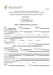
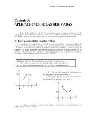
Chapter 2The TOPSPIN Interface2.1 The Topspin WindowThe TOPSPIN window consist of several areas, bars, fields and buttons. The mainpart is a split pane which consists of the data area and the browser. Note that thebrowser can be inactive [hit Ctrl+d] or displayed as a separate window.Fig. 2.1 shows the Topspin window with two data windows in the data area and thebrowser as an integral part.

28 The TOPSPIN InterfacemenubaruppertoolbarlowertoolbarDONEtitle barINDEXINDEXminimizebuttonmaximizebuttonclosebuttonbrowserdataareascrollarrowscommand linestatus bar1D data window2D data windowFigure 2.1Note that the menus and toolbars depend on the data dimensionality. The descriptionsbelow hold for 1D data. For 2D and 3D data, the menus and toolbars are similarand will be discussed in the chapters 9, 10 and 12, respectively.How to Use Multiple Data WindowsTOPSPIN allows you to use multiple data windows. Data windows can be openedfrom the browser or from the Window menu. They can contain the same of differentdatasets. Data windows can be arranged from the Window menu. One ofthem is the active (current) data window. The active window:

The TOPSPIN Interface 29• can be selected by clicking inside the window or hitting F6 repeatedly.• has a highlighted title barINDEX• has the mouse focus• is affected INDEX by menu, toolbar DONEand command line commandsA cursor line (1D) or crosshair (2D) is displayed in all data windows at the sameposition. Moving the mouse affects the cursor in all data windows.How to Use the Title barIn the title bar you can:• Left-click-hold & drag to move the window• Double-click to maximize the window• Right-click to open the title bar menu.• Access the minimize, maximize and close buttons at the right• Access the title bar menu button at the leftHow to Use the Menu barThe menu bar contains the following menus:• File : performing data/file handling tasks• Edit : copy & paste data and finding data• View : display properties, browser on/off, notebook• Spectrometer : data acquisition and acquisition related tasks• Processing : data processing• Analysis : data analysis• Options : setting various options, preferences and configurations• Window : data window handling/arrangement• Help : access various manuals.Experienced users will usually work with keyboard commands rather than menucommands. Note that the main keyboard commands are displayed in squarebrackets [] behind the corresponding menu entries. Furthermore, right-clickingany menu entry will show the corresponding command.

30 The TOPSPIN InterfaceHow to Use the Upper ToolbarThe upper toolbar contains buttons for data handling, switching to interactivemodes, display settings, and starting acquisition. INDEXButtons for DONE data handling: INDEXThe functions of the individual buttons are:Create a new dataset[Ctrl+n, new]Open a dataset [Ctrl+o, open]Save the current dataset [Ctrl+s, sav]Email the current dataset[smail]Print the current dataset [Ctrl+p, print]Copy the data path of the active data window to the clipboard [copy]Paste the data path on the clipboard to the active data window [paste]Switch to the last 2D dataset [.2d]Switch to the last 3D dataset [.3d]For more information on dataset handling, please refer to chapter 4.3.Buttons for interactive manipulationThe functions of the individual buttons are:Switch to phase correction modeSwitch to calibration modeSwitch to baseline correction mode

The TOPSPIN Interface 31Switch to peak picking modeSwitch INDEX to integration modeSwitch INDEX to multiple display DONEmodeSwitch to distance measurement modeFor more information on interactive manipulation, refer to chapter 11 and 12.Buttons for display optionsThe functions of the individual buttons are:Toggle between Hz and ppm axis unitsSwitch the y-axis display between abs/rel/offSwitch the overview spectrum on/offToggle grid between fixed/axis/offFor more information on display options, please refer to chapter 8.5 and 9.5.How to Use the Lower ToolbarThe lower toolbar contains buttons for display manipulations.Buttons for vertical scaling (intensity manipulation)Increase the intensity by a factor of 2 [*2]Decrease the intensity by a factor of 2 [/2]Increase the intensity by a factor of 8 [*8]Decrease the intensity by a factor of 8 [/8]

32 The TOPSPIN InterfaceIncrease/decrease the intensity smoothlyReset the intensity [.vr] INDEXButtons for horizontal DONE scaling (zooming): INDEXReset zooming (horizontal scaling) to full spectrum [.hr]Reset zooming (horizontal scaling) and intensity (vert. scaling) [.all]Zoom in (increase horizontal scaling) [.zi]Zoom in/out smoothlyZoom out (decrease horizontal scaling) [.zo]Exact zoom via dialog box[.zx]Retrieve previous zoom [.zl]Retain horizontal and vertical scaling when modifying dataset orchanging to different dataset. Global button for all data windows[.keep]Buttons for horizontal shiftingShift to the left, half of the displayed region [.sl]Smoothly shift to the left or to the rightShift to the right, half of the displayed region [.sr]Shift to the extreme left, showing the last data point [.sl0]Shift to the extreme right, showing the first data point [.sr0]

The TOPSPIN Interface 33Buttons for vertical shiftingINDEXShiftINDEXthe spectrum baselineDONEto the middle of the data field [.su]Smoothly shift the spectrum baseline up or down.Shift the spectrum baseline to the bottom of the data field [.sd]2.2 Command Line UsageHow to Put the Focus in the Command LineIn order to enter a command on the command line, the focus must be there. Notethat, for example, selecting a dataset from the browser, puts the focus in thebrowser. To put the focus on the command line:! Hit the Esc keyor! Click inside the command lineHow to Retrieve Previously Entered CommandsAll commands that have been entered on the command line since TOPSPIN wasstarted are stored and can be retrieved. To do that:! Hit the ↑ (Up-Arrow) key on the keyboardBy hitting this key repeatedly, you can go back as far as you want in retrievingpreviously entered commands. After that you can go forward to more recently enteredcommands as follows:! Hit the ↓ (Down-Arrow) key on the keyboardHow to Change Previously Entered Commands1. Hit the ← (Left-Arrow) or → (Right-Arrow) key to move the cursor2. Add characters or hit the Backspace key to remove characters3. Mark characters and use Backspace or Delete to delete them, Ctrl+c

34 The TOPSPIN Interfaceto copy them, or Ctrl+v to paste them.In combination with the arrow-up/down keys, you can edit previously enteredcommands.INDEXDONE INDEXHow to Enter a Series of CommandsIf you want to execute a series of commands on a dataset, you can enter the commandson the command line separated by semicolons, e.g.:em;ft;apkIf you intend to use the series regularly, you can store it in a macro as follows:! right-click in the command line and choose Save as macro.2.3 Command Line HistoryTOPSPIN allows you to easily view and reuse all commands, which were previouslyentered on the command line. To open a command history control window;click View " Command Line History, or right-click in the commandline and choose Command Line History, or enter the command cmdhist(see Fig. 2.2).It shows all commands that have been entered on the command line since TOP-SPIN was started. You can select one or more commands and apply one of the followingfunctions:ExecuteExecute the selected command(s).AppendAppend the (first) selected command to the command line. The appendedcommand can be edited and executed. Useful for commands with manyarguments such as re.Save as..The selected command(s) are stored as a macro. You will be prompted forthe macro name. To edit this macro, enter edmac . To executeit, just enter its name on the command line.

The TOPSPIN Interface 35INDEXINDEXDONEFigure 2.22.4 Starting TOPSPIN commands from a Command PromptTOPSPIN commands can be executed from a Windows Command Prompt or LinuxShell. To do that:1. Open a Windows Command Prompt or Linux Shell2. Enter a Topspin command in the following format:\prog\bin\sendgui where is the TOPSPIN installation directory.

36 The TOPSPIN InterfaceExamples:C:\ts1.3\prog\bin\sendgui re exam1d_1H 1 1 C:/bio joeINDEXreads the dataset C:/bio/joe/nmr/exam1d_13C/1/pdata/1.DONE INDEXC:\ts1.3\prog\bin\sendgui ftexecutes a 1D Fourier transform.Commands are executed on the currently active data window.2.5 Function Keys and Control KeysFor several TOPSPIN commands or tasks, you can use a control-key or function-keyshort cut.Focus anywhere in TOPSPINEsc Put the focus in the command lineShift+Esc Display menu bar and toolbars (if hidden)F2 Put the focus in the browser / portfolioF1 Search for string in command help or NMR Guide[help]F6 Select the next window in the data areaAlt+F4 Terminate TOPSPIN [exit]Ctrl+d Switch the browser/portfolio on/offCtrl+o Open data [open]Ctrl+f Find data [find]Ctrl+n New data [new]Ctrl+p Print current data [print]Ctrl+s Save current data [sav]Ctrl+w Close active window [close]Ctrl+c Copy a text that you selected/highlighted in an errorbox, dialog box, pulse program, title etc., to theclipboardCtrl+v Paste text from the clipboard into any editable field.

The TOPSPIN Interface 37Focus in the Command LineCtrl+Backspace Kill current inputCtrl+Delete INDEX Kill current inputINDEXUpArrow SelectDONEprevious command (if available).DownArrow Select next command (if available).Focus in the Browser/PortfolioUpArrow Select previous datasetDownArrow Select next datasetEnter In the Browser: expand selected nodeEnter In the Portfolio: display selected dataFocus anywhere in TOPSPINScaling DataAlt+PageUp Scale up the data by a factor of 2 [*2]Alt+PageDown Scale down the data by a factor 2 [/2]Ctrl+Alt+PageUp Scale up by a factor of 2, in all data windowsCtrl+Alt+PageDown Scale down by a factor of 2, in all data windowsAlt+Enter Perform a vertical resetCtrl+Alt+Enter Perform a vertical reset in all data windowsZooming dataAlt+Plus Zoom in [.zi]Alt+Minus Zoom out [.zo]Ctrl+Alt+Plus Zoom in, in all data windowsCtrl+Alt+Minus Zoom out, in all data windowsShifting DataAlt+UpArrow Shift spectrum up [.su]Alt+DownArrow Shift spectrum down [.sd]Alt+LeftArrow Shift spectrum to the left [.sl]Alt+RightArrow Shift spectrum to the right [.sr]Ctrl+Alt+UpArrow Shift spectrum up, in all data windowsCtrl+Alt+DownArrow Shift spectrum down, in all data windowsCtrl+Alt+LeftArrow Shift spectrum to the left, in all data windowsCtrl+Alt+RightArrow Shift spectrum to the right, in all data windows

38 The TOPSPIN InterfaceFocus in a Table (e.g. peaks, integrals, nuclei, solvents)delete Delete the selected entrieshome Select the first entryINDEXend SelectDONEthe last entryINDEXShift+Home Select the current and first entry and all in betweenShift+End Select the current and last entry and all in betweenDownArrow Select next entryUpArrow Select previous entryCtrl+a Select all entriesCtrl+c Copy the selected entries to the clipboardCtrl+z Undo last actionCtrl+y Redo last undo actionFocus in a Plot EditorF1 Open the Plot Editor ManualF5 Refreshctrl+F6 Display next layoutctrl+Shift+F6 Display previous layoutCtrl+tab Display next layoutdelete Delete the selected objectsCtrl+a Select all objectsCtrl+i Open TOPSPIN InterfaceCtrl+c Copy the selected object from the ClipboardCtrl+l Lower the selected objectCtrl+s Save the current layoutCtrl+m Unselect all objectsCtrl+n Open a new layoutCtrl+o Open an existing layoutCtrl+p Print the current layoutCtrl+r Raise the selected objectCtrl+t Reset X and Y scaling of all marked objectsCtrl+v Paste the object from the ClipboardCtrl+w Open the attributes dialog window.Ctrl+x Cut the selected object and place it on the ClipboardCtrl+z Undo the last actionNote that the function of function keys can be changed as described in chapter2.7.

The TOPSPIN Interface 392.6 Help in TopspinTOPSPIN offers help INDEX in various ways like online manuals, command help and tooltips.INDEX DONEHow to Open Online Help documentsThe online help manuals can be opened from the Help menu. For example, toopen the manual that you are reading now:! Click Help " User’s GuideTo open the Avance Beginners Guide guide:! Click Help " Avance Beginners GuideTo open the Processing Reference guide:! Click Help " Processing Reference ManualNote that most manuals are stored in the directory:/prog/docu/english/xwinproc/pdfThe most recent versions can be downloaded from:www.bruker-biospin.deHow to Get TooltipsIf you hold the cursor over a button of the toolbar, a tooltip will pop up. This is ashort explanation of the buttons function. For example, if you hold the cursor overthe interactive phase correction button, you will see the following:The corresponding command line command, in this case .ph, is indicated betweensquare brackets.Note that the tooltip also appears in the status bar at the bottom of the TOPSPINwindow.

40 The TOPSPIN InterfaceHow to Get Help on Individual CommandsTo get help on an individual command, for example ft:INDEX! Enter ft?DONE INDEXor! Enter help ftIn both cases, the HTML page with a description of the command will be opened.Note that some commands open a dialog box with a Help button. Clicking thisbutton will show the same description as using the help command. For example,entering re and clicking the Help button in the appearing dialog boxopens the same HTML file as entering help re or re?.How to Use the Command IndexTo open the TOPSPIN command index:! Enter cmdindexor! Click Help " Command IndexFrom there you can click any command and jump to the corresponding help page.

The TOPSPIN Interface 412.7 User Defined Functions KeysThe default assignment INDEXof functions keys is described in chapter 2.5 and in thedocument:INDEX DONE! Help " Control and function keysYou may assign your own commands to functions keys. Here is an example of howto do that:1. Open the file cmdtab_user.prop, located in the subdirectory userdefinedof the user properties directory (to locate this directory, enter histand look for the entry "User properties directory=" ). The filecmdtab_user.prop is initially empty and can be filled with your owncommand definitions.2. Insert e.g. the following lines into the file:_f3=$em_f3ctrl=$ft_f3alt=$pk_f5=$halt_f5ctrl=$reb_f5alt=$popt3. Restart TOPSPINNow, when you hit the F3 key, the command em will be executed. In the sameway, Ctrl+F3, Alt+F3, F5, Ctrl+F5 and Alt+F5 will execute the commandsft, pk, halt, reb and popt, respectively. You can assign any command,macro, AU program or Python program to any function keys. Only thekeys Alt+F4, F6, Ctrl+F6, and Alt+F6 are currently fixed. Their functioncannot be changed.2.8 How to Open Multiple TOPSPIN InterfacesTOPSPIN allows you to open multiple User Interfaces. This is, for example, usefulto run an acquisition in one interface and process data in another. To open an additioninterface, enter the command newtop on the command line or click Window" New Topspin. To open yet another interface, enter newtop in the first or in thesecond interface. The display in each interface is completely independent from theothers. As such, you can display different datasets or different aspects of the same

dataset, e.g. raw/processed, regions, scalings etc. When the dataset is (re)processedin one interface, its display is automatically updated in all TOPSPIN interfaces.The command exit closes the current Topspin interface. Interfaces that wereopened from this interface remain open. Entering exit in the last open TOPSPINinterface, finishes the entire TOPSPIN session. The position and geometry of eachTOPSPIN interface is saved and restored after restart.

Chapter 3Trouble Shooting3.1 General Tips and TricksOn a spectrometer, make sure the commands cf and expinstall have beenexecuted once after installing TOPSPIN. cf must be executed again if your hardwareconfiguration has changed. Sometimes, executing cf is useful in case ofacquisition problems.On a datastation, a default configuration is automatically done during the installation.No configuration commands are required. Only if you want to use AU programs,you must run expinstall once.3.2 History, Log Files, Stack TraceIf you have a problem with TOPSPIN and want to contact Bruker, it is useful to haveas much information as possible available. If TOPSPIN is still running, you can viewlog files with the commands hist and ptrace. If TOPSPIN hangs, you can createa stack trace by hitting Ctrl+\ (Linux) or Ctrl+Break (Windows) in the TOP-SPIN startup window.

44 Trouble Shooting3.2.1 History log fileBy default, the history (protocol) feature is switched on.This means all TOPSPINcommands will be protocolled and can be examinedINDEXby entering hist on the commandline.DONE INDEXIf, for some reason, history is switched off, you can switch it on as follows:1. Click Options " Preferences, click Miscellaneous2. Check the entry "Record commands in protocol file"3. Click OK.3.2.2 All log filesA full protocol including not only TOPSPIN commands but also dataserver and networktraffic is show by the command ptrace. This opens the following dialog

Trouble Shooting 45window:INDEXINDEXDONEFigure 3.1Here TOPSPIN log messages from various log files are displayed time sorted.

46 Trouble ShootingMessages from different log files are shown in different colours. The color assignmentand location of the files is shown in the lower part of the dialog window.ptrace supports the following functions: INDEXDONE INDEXSearch keywordsTo search the displayed log files for a certain keyword, just enter it in the textbar at the top of the window and hit Enter.Anchor specific entriesTo anchor an entry:double-click in the first column of the entryThe entry is marked with an X. Now you can use the < > buttons at the upperright of the window to go to the previous or next entry, respectively.Add log filesBy default, the procol.txt, history and dataserver log files areshown.To include additional log files to the ptrace list:click File " Add, specify the file and click Open.Note that most log files are stored in the directory:/prog/curdir/Save the log messagesTo save log messages in a text file;click File " Save and specify the output text file3.2.3 Create a Stack TraceIf TOPSPIN hangs it can be useful to sent Bruker a stack trace about a possiblecause. You can create a stack trace as follows.1. Move the cursor into the TOPSPIN startup window.2. Under Windows: hit Ctrl+Break (=Ctrl+Pause)Under Linux: hit Ctrl+\ (Control backslash)3. Copy the appearing text into a text file.

Trouble Shooting 473.3 How to Show or Kill TOPSPIN processesTo show the currently INDEXrunning TOPSPIN processes, enter the command show orkill on the command line. A list of processes will appear showing the processINDEX DONEcommand, dataset etc.Figure 3.2Fig. 3.2 shows a list with one process (command xfb). To kill a process, select itin the list and click the button Kill...The command show all or kill all work like show and kill, except thatthey also show TOPSPIN system processes. Note that killing such processes maykill TOPSPIN.3.4 What to do if TOPSPIN hangsIf, for some reason, TOPSPIN hangs, please do the following.Under Linux:1. Open a Shell2. Enter /prog/bin/script/killtopspinwhere is the TOPSPIN installation directory.Under Windows:1. Click Start " Programs " Bruker TOPSPIN " TOPSPIN 1.3 " BrukerUtilities 1.32. In the appearing window:

48 Trouble ShootingClick killtopspin.Normally, this kill all TOPSPIN processes including cpr, cprserver, dataserver andjava.INDEXDONE INDEX3.5 How to Restart User Interface during AcquisitionIf Topspin hangs up during a data acquisition, you can restart the user interfacewithout disturbing the acquisition. To do that:1. Open the file:/prog/curdir//historywhere is the TOPSPIN home directory and is the user whostarted TOPSPIN. Look for the term ’Java Virtual Machine’ and check its PID.2. Open the Task Manager (Windows) or System Monitor (Linux)3. Stop the Java(w).exe process with the PID found in the history file.4. Open a Windows Command Prompt or Linux Shell5. Go to the TOPSPIN Installation directory6. Enter topspin -client

Chapter 4Dataset Handling4.1 The Topspin Browser and PortfolioTOPSPIN offers a data browser/portfolio from which you can browse, select, andopen data. Furthermore it allows you to define and list alias names for data. Thebrowser appears at the left of the TOPSPIN window and can be controlled from theView menu.The browser is similar to the Windows Explorer. It shows data directory trees andallows you to expand/collapse their elements. Figure 4.1 shows a TOPSPIN browserwith one top level data directory and one dataset fully expanded.

50 Dataset Handling:INDEXDONEINDEXFigure 4.1The TOPSPIN portfolio shows the list of datasets that has been opened so far by thecurrent user. Each dataset that you open, is automatically added to the current portfolio.A portfolio with five datasets look like this:Figure 4.2Each line displays one dataset showing its name, expno, procno, top level directoryand user.The TOPSPIN Alias list show a list of alias names for datasets. Just right-click any

Dataset Handling 51entry to define, remove or interpret alias names.INDEXINDEXDONEFigure 4.3How to Open the Browser/Portfolio! Click View " Browser Panel On/Off [Ctrl+d]The browser or portfolio will appear depending on which one was used last.How to Open the Browser/Portfolio in a separate windowThe browser or portfolio can be opened in a separate window as follows:! Click Options " Preferences [set], click Window settings and check Displaydataset browser in a separate window.You must restart TOPSPIN for the change to take effect.How to Put the Focus in the Browser/Portfolio! Hit the F2 keyor! Click inside the browser or portfolioHow to Select Folders in the BrowserTo select a particular folder:! Left-click the folder buttonor! Hit the arrow-up/down keys while the focus is in the browserTo select multiple folders:

52 Dataset Handling! Hold the Ctrl key and left-click multiple folders to select themorINDEX! Hold the Shift key and left-click two folders to select these two and allin between. DONE INDEXHow to Expand/Collapse a Folder in the BrowserTo expand a collapsed folder:! Click the + button to the left of the folder buttonor Double-click the folder buttonor Hit the Right-Arrow key while the folder is highlightedor Right-click the folder button and choose Expand fully from the popupmenu to fully expand the folderTo collapse an expanded folder:! Click the - button to the left of the folder buttonor Double-click the folder buttonor Hit the Left-Arrow key while the folder is highlightedHow to Expand a Folder showing Pulse program and Title! Right-click the data name folder button and chooseExpand fully & show PULPROG /Title from the popup menuFig. 4.4 shows an example of an expanded dataset showing the pulse programand title.Figure 4.4

Dataset Handling 53Note that collapsing the data name folder will deselect the display of the pulseprogram and title.INDEXHow to Add/Remove a Top Level Data DirectoryINDEX DONETo add a new top level data directory, local or remote, to the browser:1. Right-click any position in the browser2. Choose Add new data dir... from the popup menu (see Fig. 4.5)3. Enter the top level directory in the dialog box and click OKTo remove an existing top level directory from the browser:1. Right-click the folder button of the top level directory2. Choose Remove selected data dir... from the popup menu (see Fig. 4.5)Figure 4.53. Click OK to confirm the appearing messageBy default, the browser shows the TOPSPIN installation directory with the Brukerexample datasets. To suppress this feature click Options " Preferences [set],click Program startup actions and uncheck Show TOPSPIN default data directoryin data browser.How to Open a New Portfolio1. Right-click inside the portfolio

54 Dataset Handling2. Choose Open portfolio... from the appearing popup menu (see Fig. 4.6)3. Navigate to the folder that contains the portfolio filesINDEX4. Select the desired portfolio file (extension .prop)5. Click OpenDONE INDEXHow to Save the current Portfolio1. Right-click inside the portfolio.2. Choose Save portfolio... from the appearing popup menu (see Fig. 4.6).3. Specify a folder and filename in the appearing dialog box. The filenamemust have the extension .prop.4. Click Save.How to Remove Datasets from the PortfolioTo remove a single dataset from the portfolio:1. Right-click the dataset.2. Choose Remove from portfolio...from the popup menu (see Fig. 4.6).3. Click OK in the appearing alert box.To remove multiple datasets from the portfolio:1. Hold the Ctrl key and left-click several datasets to select them or holdthe Shift key and left-click two datasets to select these two and all inbetween.2. Right-click any of the selected datasets.3. Choose Remove from portfolio...from the popup menu (see Fig. 4.6).4. Click OK in the appearing alert box.How to Find Data and Add them to the Portfolio1. Click Edit " Find data [Ctrl+f | find].2. Specify the search criteria and click OK.3. Select dataset(s) and click Add to portfolio.How to Sort Data in the Portfolio1. Right-click inside the portfolio

Dataset Handling 552. Choose Sort mode from the popup menu (see Fig. 4.6).3. Click Alphabetical to sort data in alphabetical orderINDEXorClick RecentINDEXfirst to sortDONEdata by date of last open.Figure 4.6How to Add, Remove or Interpret Alias NamesTo add an alias name:1. Click the Alias tab in the browser.

56 Dataset Handling2. Right-click in the Alias table to open the popup menu (see Fig. 4.7).INDEXDONEINDEX3. Click Define alias names for data in selected window.4. Enter an alias name in the appearing dialog box and click OK. Note thatalias names must begin with a letter.To remove an alias name:1. Right-click the alias name2. Click Remove selected aliases... from the popup menu (see Fig. 4.7)Furthermore, the popup menu offers entries to display the dataset, list its propertiesand print the full dataset specification.4.2 Creating DataFigure 4.7How to Create a New Dataset1. Click File " New [new , Ctrl+n]orClick the button in the upper toolbar.2. Specify the dataset name, expno, procno, dir, and user in the appearing dialogbox. If one or more datasets are open, the fields are initialized with thecurrent dataset (see Fig. 4.8).

Dataset Handling 573. Click the down-arrow of the Solvent box and choose a solvent from the list,or type a solvent name.4. Click the INDEX down-arrow of the Experiment box and choose a parameter setfrom the list, or type a parameter set name.INDEX DONE5. Type the dataset title in the TITLE box.6. Click OK.A dataset will be created and initialized with the parameters of the chosen experiment.No fid or spectrum are available yet. They can be created by data acquisitionand data processing, respectively.4.3 Opening DataFigure 4.8TOPSPIN allows you to open data in several ways, from the browser, the menu, the

58 Dataset HandlingExplorer or the command line. Furthermore, data can be opened:• in an existing data window replacing the current dataset.INDEX• in a data window which is in multiple display mode, being superimposed onthe current spectra. DONE INDEX• in a new data window which becomes the active window.Note that if a dataset is already displayed in one window and it is opened in a secondexisting window, it still replaces the dataset in the latter one. As a result, thesame dataset will be displayed in two windows (see also command reopen).How to Open Data Windows CascadedBy default, a new data window appears maximized, filling the entire data field andcovering possibly existing window. You can, however, configure TOPSPIN to opennew windows cascaded. This is convenient if you want to open several data windowsand then select one.To open new windows cascaded:1. Click Options " Preferences [set]2. Click Window Setting in the left part of the dialog box.The right part of the dialog box shows the window settings (see Fig. 4.9).Figure 4.93. Check Open new internal windows ’cascaded’ rather than ’max’.4. Optionally you can configure the cascaded windows by clicking the respectiveChange button. This will open the dialog box shown in Fig. 4.10.

Dataset Handling 59INDEXINDEXDONEFigure 4.105. Here you can specify the data window sizes and offsets as fractions of themaximum window sizes.6. Click OK to close the dialog box.How to Open Data from the BrowserIn the browser:! Left-click-hold a data name, expno or procno and drag it into the data area.The data will be displayed in a new data window.or Left-click-hold a data name, expno or procno and drag it into an open datawindow. The data will replace the currently displayed data.or Left-click-hold a data name, expno or procno and drag it into an empty datawindow created with Alt+w n.or Left-click-hold a data name, expno or procno and drag it into a multiple displaydata window. The data will be superimposed on the currently displayeddata.or Right-click a data name, expno or procno and choose Display from the popupmenu; the data will be displayed in the current data window.or Right-click a data name, expno or procno and choose Display in new win-

60 Dataset Handlingdow from the popup menu; the dataset will be displayed in a new data window.or Hold the Ctrl key and left-click several INDEX datasets to select them or hold theShift key and left-clickDONEtwo datasets toINDEXselect these two and all in between.Then right-click one of the selected datasets and choose Displayfrom the popup menu. A new window will be opened showing the selecteddatasets in multiple display mode. However, if the current window was alreadyin multiple display mode, the selected spectra will be superimposedon the currently displayed spectra.How to Open Data from the PortfolioThe portfolio offers the same possibilities to open a dataset as the browser. Additionaloptions are:! Hit the Enter key to display the highlighted dataset in the current window.Figure 4.11! Double-click a dataset to display it in the current window.How to Automatically Select the first expno/procno of a datasetIf you open a dataset from the Browser by clicking a data name, there might bemore that one expno and/or procno available. By default, TOPSPIN then opens adialog box from which you can select the desired expno/procno combination (seeFig. 4.12). You can, however configure TOPSPIN to automatically open the firstavailable expno/procno combination. To do that:1. Click Options " Preferences [set].2. Click Miscellaneous in the left part of the dialog box.3. Uncheck the item Display expno/procno list when opening data.4. Click OK to close the dialog box.

Dataset Handling 61INDEXINDEXDONEFigure 4.12How to Open Data from the Topspin menu1. To open a dataset:! Click the button in the upper toolbar.or! Click File " Open [open, Ctrl+o] (see Fig. 4.13).

62 Dataset HandlingINDEXDONEINDEXFigure 4.132. In the appearing dialog box (see Fig. 4.14):Figure 4.14a) Select the option Open NMR data stored in standard Bruker format.b) Select the browser type RE Dialog.c) Click OK.

Dataset Handling 633. In the appearing dialog box (see Fig. 4.15).:INDEXINDEXDONEFigure 4.15a) Specify the dataset name, expno etc.b) Click OK.Note that the dataset specification consists of the five variable parts of the datadirectory tree, in this case:C:\bio\data\guest\nmr\exam1d_1H\1\pdata\1The text boxes are initialized with the dataset in the current data window.How to Open Data from the Explorer, Konqueror or NautilusYou can open a dataset from the Windows Explorer as follows:1. Open the Windows Explorer. You can do that in two different ways:! from the Windows Start button. Navigate to the data name, expno orprocno.or! by entering the command expl in TOPSPIN. The Explorer shows the contentsof the current dataset procno directory. Navigate to the desired dataname, expno or procno. expl can also be used with the argument topto open the TOPSPIN installation directory, home to open user home directoryor with an absolute pathname to open that directory.2. Now you can open a dataset with:

64 Dataset Handling! drag & drop: click-hold a dataset name or any of its sub-folders or filesand drag it into the TOPSPIN data area or data window.orINDEX! copy & paste: right-click DONE a dataset and INDEX choose copy from the popupmenu. In TOPSPIN, click Edit " Paste [paste] (see Fig. 4.16).Figure 4.16Likewise, a dataset can be opened from the Windows Search window or InternetBrowser.How to Open Data from the Command LineTo open a dataset from the command line:1. Enter re2. Specify a dataset in the appearing dialog box (see Fig. 4.15).3. Click OKTo open a new procno of the current dataset:1. Enter rep2. Specify a procno in the appearing dialog box.3. Click OKTo open a dataset in a new window:1. Enter rew2. Specify a dataset in the appearing dialog box.3. Click OKTo open a new procno of the current dataset in a new window:1. Enter repw

Dataset Handling 652. Specify a procno in the appearing dialog box.3. Click OKINDEXTo open a data browser and read a dataset from there:1. Enter reb INDEX DONE2. Select a dataset from the appearing dialog box.3. Click DisplayNote that re, rep and reb:• Replace the data in the currently selected data window.• Open the data in a new window when they are used after typing Alt+w n• Add the data in the currently selected window if this is in multiple displaymode.whereas rew and repw :• Always open the dataset in a new window.How to Open Special Format DataApart from the standard Bruker data format, TOPSPIN is able to read and displayvarious other formats. To do this:! Click File " Open [open, Ctrl+o]select the option Open NMR data stored in special formats, select the desired filetype (see Fig. 4.17) and click OK..A dialog will appear which depends on the chosen file type. Just follow the instructionson the screen.The following file types are supported:• JCAMP-DX - Bruker TOPSPIN 1 data stored in JCAMP-DX format• Zipped TOPSPIN - Bruker TOPSPIN data stored in ZIP format• WINNMR - Bruker WINNMR data• A3000 - Bruker Aspect 3000 data1. Note that the TOPSPIN data format is identical to the XWIN-NMR data format.

66 Dataset Handling• VNMR - data acquired on a Varian spectrometer• JNMR - data acquired on a Jeol spectrometerINDEX• Felix - 1D data, FID or spectrum, which are stored in FELIX format.Note that in all cases, the data are DONE stored in a single INDEX data file which is unpacked/convertedto standard Bruker format, i.e. to a data directory tree.How to Open a ZIP or JCAMP-DX file from the Windows ExplorerData stored in ZIP or JCAMP-DX format can also be opened directly from theWindows Explorer. You can do that as follows:! drag & drop: click-hold a file with the extension .dx or .zip and dragit into the TOPSPIN data area or data window.! copy & paste: right-click a file with the extension .dx or .zip andchoose copy from the popup menu. In TOPSPIN, click Edit " Paste[paste].4.4 Saving/Copying DataFigure 4.17How to Save or Copy DataYou can save the current dataset as follows:

Dataset Handling 671. Click File " Save [Ctrl+s].This will open a dialog box (see Fig. 4.18).INDEXINDEX DONEFigure 4.182. Select an option and, if applicable, a file type.3. Click OK to execute the option.The six options correspond to the following command line commands:• wrpa - copies the current data to a new data name or expno• tozip - convert a dataset of any dimension to ZIP format• tojdx - convert a 1D or 2D dataset to JCAMP-DX format• totxt - convert a 1D or 2D dataset text format• wpar - write parameter set• convdta - save digitally filtered data as analog filtered data• wrp, wra, genfid, wmisc - write various filesHow to Save an Entire Dataset1. Click File " Save [Ctrl+s].

68 Dataset Handling2. Select the option Copy dataset to a new destination [wrpa] and click OK3. Specify the dataset variables and click OKINDEXHow to Save Processed DataDONE INDEX1. Click File " Save [Ctrl+s].2. Select the option Save other file3. Select File type Processed data as new procno [wrp] and click OK4. Enter a processing number (procno) and click OKHow to Save Acquisition Data1. Click File " Save [Ctrl+s].2. Select the option Save other file3. Select File type Acqu. data as new expno [wra] and click OK4. Enter a experiment number (expno) and click OKHow to Save Processed Data as Pseudo Raw Data1. Click File " Save [Ctrl+s]2. Select the option Save other file3. Select File type 1r/1i as fid [genfid] or 2rr/2ii as ser [genser]4. Click OK5. Enter a destination expno.(optionally, you can specify further data path specifications)6. Click OK4.5 Deleting DataHow to Delete a Specific Dataset! Right-click the data name, expno or procno in the browser, then click Delete...In each case, a delete dialog will appear. The dialog box for a data expno, for anis shown in Fig. 4.19.

Dataset Handling 69INDEXINDEXDONEYou can choose to delete just the raw data, delete the entire expno with all procnosor open further delete options. In the later case, the dialog box shown in Fig. 4.20will appear.How to Delete Types of DatasetsTo delete certain types of data like 1D raw data, 2D processed data etc.:! Click File " Delete...orFigure 4.19! Enter delete on the command line.The dialog window shown in Fig. 4.20 will appear. Here you can select the datatype and selection criteria.

70 Dataset Handling:INDEXDONEINDEXFigure 4.201. Select a data type optionFor each option, the corresponding command appears in the title of the dialogbox. These commands can also be used to delete data from the command line.2. Specify the Required parametersNote that you can use the wildcards:• Asterix (*) for any character and any number of characters.• Question mark (?) for any single character.3. Click OKA dialog box will appear showing the matching datasets. For example, if you selectthe option An entire dataset ... :1. Select dataset entries for deletion (selected entries are highlighted).

Dataset Handling 71To select multiple entries: click them holding the Shift or Ctrl key.2. Click Delete to delete the entire data directory.INDEXIf you select the option Acquisition data or Processed data, you can choose betweendeleting INDEX the data files DONE only and deleting the entire expno or procno directory,respectively (see Fig. 4.21).4.6 Searching/Finding DataFigure 4.21How to Find DataYou can find TOPSPIN data according to various criteria. To start searching do thefollowing:1. Click Edit " Find data [Ctrl+f | find]to open the Find data window (see Fig. 4.22).

72 Dataset HandlingINDEXDONEINDEXFigure 4.222. Specify the search criteria. Note that:• Dataset variables are searched that contain the specified string.• Search is restricted to data created between the specified dates. Note thatthe acquisition date is evaluated.The Reset mask button resets the default criteria.3. Click OKto get a list of data that fulfil these criteria (see Fig. 4.23).

Dataset Handling 73INDEXINDEXDONEFigure 4.23Note that the current search criteria are preserved until you exit TOPSPIN.How to Display one of the Found DatasetsIn the search result window (see Fig. 4.23):1. Click one dataset to select it.Optionally: click Properties to view the datasets properties.2. Click Displayto display the selected dataset in the current data window.Note that if the search result consist of only one dataset, this is automatically selectedand you can skip step 1.How to Select Data from the Found DatasetsIn the search result window (see Fig. 4.23):

74 Dataset Handling! Hold the Ctrl key and left-click several datasets to select these datasets.orINDEX! Hold the Shift key and left-click two datasets to select these datasets andall datasets in between. DONE INDEXor! Click Select all to select all datasets in the search result.How to Add Selected Datasets to the Portfolio1. Select the desired dataset(s) as described above.2. To add them to the portfolio:! Click Add to portfolio to extend the current portfolio.or! Click Replace portfolio to replace the current portfolio.How to Save Selected Datasets to a List1. Select the desired dataset(s) as described above.2. Click Save selection...3. In the appearing browser:a) Navigate to the desired list directory.b) Enter or select the list filename.c) Click OKDataset lists can be used by the acquisition or by serial processing (commandserial).4.7 Handling Data FilesHow to List/Open the Current Dataset FilesA Bruker dataset is represented by a directory tree which contains files in the expnoand procno subdirectories. These files contain the actual data, parameters,lists etc.

Dataset Handling 75! Right-click inside the data window and choose Files from the popup menu.INDEXINDEXDONEIf the spectrum is displayed, the files in the procno subdirectory areshown. If the Fid is displayed, the files in the expno subdirectory areshown.! Select a file and click Open to view its contents.Note that this only makes sense for ascii files.How to List/Open the current Dataset Files in the Windows ExplorerTo list the current dataset files in the Windows Explorer:1. Click Files " Run...2. Select Open file explorer [expl] in the appearing dialog box3. Click OKAlternatively, you can enter the command expl on the command line. The WindowsExplorer will be opened showing the processed data files (the files in theprocno directory) of the current dataset. Under Linux a Web browser like KDE

76 Dataset HandlingKonqueror or Gnome Mozilla will be opened.To open a file:INDEX! Double-click the file or right-click the folder icon and choose OpenDONE INDEXIf TOPSPIN data area contains no datasets, the expl command opens the Explorershowing the users home directory. When entered on the command line, expl canalso be used with the argument top to open the TOPSPIN installation directory,home to open user home directory or with an absolute pathname to open that directory.4.8 Data Consistency CheckTOPSPIN maintains audit trail files for compliance with GLP, GMP and FDArequirements.The processing command that creates processed data from the raw data, e.g. em,creates the processing audit trail file auditp.txt and inserts the first entry. Anyprocessing command that modifies/updates the processed data, e.g. ft, makes anadditional entry. Furthermore, any command that changes one or more processingstatus parameters makes an additional entry. The audit trail can be checked withthe command audit. This command opens a dialog box (see Fig. 4.24).Figure 4.24The first two entries allow you to view the audit trail files. The third entry performsan audit trail check, i.e. a data consistency check. If both raw and processed

Dataset Handling 77data are consistent, you will get the message shown in Fig. 4.25).INDEXINDEXDONEFigure 4.25If the data have been manipulated outside of TOPSPIN, e.g. with third party software,the checksum will be inconsistent. Fig. 4.26 shows the message for inconsistentprocessed data.Figure 4.26The fourth entry in Fig. 4.24 allows you to add a comment to one of the audit trailfiles (raw or processed).

Chapter 5Parameter Handling5.1 Processing ParametersProcessing parameters can be set/changed in three different ways:• from the parameter editor: click the ProcPars tab or enter edp• from the command line: e.g. enter si• from a command dialog box: e.g. wmHow to Set a Processing Parameter from the Command LineEnter the parameter name on the command line. For example to set the size:1. Enter sifor 1D data, the following dialog box will appear:

80 Parameter Handlingfor 2D data, the following dialog box will appear:INDEXDONEINDEX2. Specify the desired value(s), e.g. 32768 or 32k3. Click OKHow to Set Processing Parameters from the Parameter EditorTo open the processing parameter editor:! Click the ProcPars tab in the Tab bar of the data window.or! Enter edp on the command line.Figure 5.1At the left of the parameter editor window you will see a list of parameter sections.The processing parameter editor supports the following functions:

Parameter Handling 81! Enter (part of) a parameter name in the search field and click .! Click a parameter section, e.g. Phase at the left of the dialog box. The sectionbecomes highlighted and the corresponding parameters will appear inINDEXthe right INDEX part of the dialog DONE box.! Click in a parameter field, e.g. PHC0, to set the parameter value.! Hit the Tab key to jump to the next parameter field.! Hit Shift+Tab to jump to the previous parameter field.! Use the scroll bar at the right of the dialog box to move to parameters furtherup or down in the dialog box.How to Undo the Last Processing Parameter Change! Click the following button:Undo last parameter change.How to Display Processing Status Parameters! Click the following button:Show processing status parameters.Note that the command dpp opens the parameter editor and automatically showsthe status parameters.How to Change Processed Data Dimensionality! Click the following button:Change data dimensionality.This changes the number of parameter columns and value of the processing parameterPPARMOD.The parameter editor does not allow you to modify status parameters. Processingstatus parameters reflect the status of the processed data and are used for furtherprocessing, display or plotting. Changing them can make the dataset inconsistent.In rare cases, however, it can be useful to change a status parameter and TOPSPINallows you to do that from the command line. If, for instance, you want to changethe F1 status parameter MC2 of a 2D dataset, you have to enter:

82 Parameter Handlings mc2Note that the command s is used for 1D, 2D and 3D dataset. TOPSPIN automaticallyrecognizes the dimensionality of the data and INDEX displays the parameter in allrelevant dimensions. Note that, forDONEexample, theINDEXparameter MC2 only exists in F1.5.2 Acquisition ParametersHow to Set Acquisition ParametersAcquisition parameters can be set/changed as follows:• from the parameter editor: click the AcquPars tab or enter eda• from the command line: e.g. enter td• from the interactive parameter adjustment window (enter gs)How to Set an Acquisition Parameter from the Command LineEnter the parameter name on the command line. For example to set the time domainsize:1. Enter tdfor 1D data, the following dialog box will appear:for 2D data, the following dialog box will appear:

Parameter Handling 832. Specify the desired value(s), e.g. 65536 or 64k3. Click OKINDEXHow to Set AcquisitionINDEXParametersDONEfrom the Parameter EditorTo open the acquisition parameter editor:! Click the AcquPars tab in the Tab bar of the data window.or! Enter eda on the command line.Fig. 5.2 shows an example of the acquisition parameter editor with the Experimentparameters displayed.Figure 5.2The processing parameter editor supports the following functions:! Enter (part of) a parameter name in the search field and click .! Click a parameter section, e.g. Experiment at the left of the dialog box. Thesection becomes highlighted and the corresponding parameters will appearin the right part of the dialog box.! Click in a parameter field, e.g. TD, to set the parameter value.! Hit the Tab key to jump to the next parameter field.! Hit Shift+Tab to jump to the previous parameter field.

84 Parameter Handling! Use the scroll bar at the right of the dialog box to move to parameters furtherup or down in the dialog box.INDEXHow to Undo the Last Acquisition Parameter ChangeDONE INDEX! Click the following button:Undo last acquisition parameter change.How to Set Pulse Program Parameters! Click the following button:Show pulse program parameters [ased]The button will change to . To make this the default setting:Click Options " Preferences, click Miscellaneous, check the entry "Showreduced parameter set (ased)" and click OK.How to Display Acquisition Status Parameters! Click the following button:Show acquisition status parameters.Note that the command dpa opens the acquisition parameter editor and automaticallyshows the status parameters.How to Get Probehead/Solvent dependent Parameters! Click the following button:Set probehead/solvent dependant parameters [getprosol].Probehead and solvent dependant parameters can be set up with the commandedprosol.How to Change Acquisition Data Dimensionality! Click the following button:Change data dimensionality.This changes the number of parameter columns and value of the acquisition parameterPARMODE.

Parameter Handling 85How to Set Lock ParametersEnter the command edlock and set the lock parameters in the appearing dialogbox. For a detailedINDEXdescription of edlock, please refer to the Acquisition Referencemanual or INDEX enter edlock? DONE on the command line.How to Set Routing ParametersEnter the command edasp and set the routing parameters in the appearing dialogbox. For a detailed description of edasp, please refer to the Acquisition Referencemanual or enter edasp? on the command line.

Chapter 6Data Processing6.1 Interactive ProcessingInteractive processing allows full control over the processing sequence. However,it requires detailed knowledge about the required parameters (see chapter 5.1) andcommands. Therefore, it is only suitable for the advanced user. New or intermediateusers are recommended to use the Processing Guide for semi-automaticprocessing (see chapter 6.2).How to Process Data with Single CommandsData can be processed by entering single commands on the command line. A typical1D processing sequence would be:em : exponential window multiplicationft : Fourier transformapk : automatic phase correctionsref : automatic calibration (referencing)abs : automatic baseline correctionThis allows you full control over each individual processing step.

88 Data ProcessingHow to Process data with Composite CommandsData can also be processed with so called composite commands. These are combinationsof single processing commands. TheINDEXfollowing composite commandsare available.DONE INDEX• ef : Exponential multiplication + Fourier transform• efp : Exponential multiplication + Fourier transform + phase correction• fmc : Fourier transform + magnitude calculation• fp : Fourier transform +phase correction• gf : Gaussian multiplication + Fourier transform• gfp : Gaussian multiplication + Fourier transform + phase correctionThey can be entered on the command line or clicked from the menu. For the latteroption:! Click Processing " More transforms " ShortcutsJust like single commands, composite commands can be used in Macros, AU programsand Python programs.6.2 Semi-automatic ProcessingHow to Use the Processing Guide in Automatic modeThe Processing Guide in automatic mode guides you through the entire processingsequence of data selection, processing, printing and archiving with minimumuser interaction.1. Click Processing " Processing GuideThe Processing Guide window will appear as an integral part of the currentdata window (see Fig. 6.1).

Data Processing 89INDEXINDEXDONEFigure 6.12. In the Processing Guide window:a) Check Automatic modeb) Click Open data set and click OK to open a dataset manually, e.g. fromthe browser or click Browse to open the File Chooser.

90 Data Processingc) Click Window function " Fourier Transform " etc.Each processing step will be executed without user interaction.INDEXHow to Use the Processing GuideDONEin InteractiveINDEXmodeThe Processing Guide in interactive mode guides you through the entire processingsequence of data selection, processing, printing and archiving requiring someuser interaction.1. Click Processing " Processing GuideThe Processing Guide window will appear as an integral part of the currentdata window.2. In the Processing Guide window:a) Uncheck Automatic modeb) Click Open data set and click OK to open a dataset manually, e.g. fromthe browser or click Browse to open the File Chooser.c) Click Window function " Fourier Transform " etc.For each step a dialog box will appear where you can enter options, parametersetc. For details on these items, please refer to the corresponding commands in theProcessing Reference Guide.6.3 Processing Data with AU programsData processing can be performed by using AU programs. An AU program is actuallya C-program which contains TOPSPIN commands (macros) and/or C-languagestatements. Various standard AU programs are delivered with TOPSPIN. A typical1D processing AU program is proc_1d. A simplified version of this AU programis:EFAPKSREFABSAUTOPLOTQUITIt executes the commands ef, apk, sref, abs and autoplot. To run this AU

Data Processing 91program, just enter proc_1d on the command line 1 . You can create your ownAU programs with the command edau. Note that an AU program must end withQUIT or QUITMSG("your INDEX message"), and that all statements must be specified incapital letters. For more information on AU programs, please refer to the AU programreference INDEX manual: DONEClick Help " Programming " AU programmingAs an alternative to AU programs, you can also write Python programs, whichallow you to use TOPSPIN commands, User Interface functions and Graphic functions.For more information:! Click Help " Programming " Python Programming6.4 Serial Processing using Python programsTOPSPIN allows you to process a series of datasets using serial scripts. The datasetlist and command(s) to be used can be easily setup from the TOPSPIN interface asfollows. Enter the command serial on the command line. This will open the1. Before you can use any Bruker AU program, expinstall must have been executed once.

92 Data Processingdialog window shown in Fig. 6.2.INDEXDONEINDEXFigure 6.2Here you can set up and start data processing of a series of datasets using scripts,which can be TOPSPIN macros or Python programs.The dialog offers you the following options:Process specified data set list with specified scriptProcess the data in the specified dataset list using the specified serial script.The flag Show data sets during script execution allows you to either displaythe currently processed dataset or remain on the current dataset.Browse for a dataset listBrowse for an existing dataset list, starting in the users home directory.Browse for a serial script

Data Processing 93Browse for existing serial script. Depending on the parameter Script type, thebrowser opens the ../exp/stan/nmr/py for Script type Python or../exp/stan/nmr/lists/mac INDEX Script type macro. TOPSPIN, by default, searches forfor files named ser_*.INDEX DONEEdit specified data set listView or edit the list specified in the field Data Set List.Edit specified serial scriptView or edit the script specified in the field Serial script nameCreate new data set listOpens a dialog box for finding datasets. Proceed as follows:1. Specify all search criteria and click OK2. In the appearing Search result box:a) Select the desired datasets.b) Click Save selection..3. In the appearing browser:a) Navigate to the desired list directory.b) Enter or select the list filename.c) Click OKAlternatively, you can create a dataset list manually.The format of a list entryis: An example of a dataset list is:exam1d_13C 1 1 C:/bio guestexam1d_13C 2 1 C:/bio guestexam1d_13C 3 1 C:/bio guestCreate new serial scriptOpens the appropriate editor to create a new script. For Script type Python,edpy is executed, for Script type macro, edmac is executed. The name of a serialscript (macro of Python) must start with ser_. Python scripts must have theextension .py. A standard example is the python script ser_efp.py.

94 Data ProcessingAn example of a simple processing sequence is exponential window multiplication,Fourier transform and automatic phase correction of a 1D dataset. A TOPSPINmacro performing this task would be: INDEXefDONEapkA Python programs performing the same task would be:EF()APK()INDEXNote that Python programs are much more versatile than macros. Details onPython programming can be found under:Help " Programming " Python programmingNote that serial processing can also be started as follows:• Click Processing " Serial Processing...or• Click File " Run, select Execute Serial script on Data set list and click OK

Chapter 7Printing/Exporting Data7.1 Printing/plotting DataHow to Print/Plot from the MenuThe current data window can be printed as follows:1. From the TOPSPIN menu:! Click the button in the upper toolbaror Click File " Printor Enter print or Ctrl+pAll these actions are equivalent; they open the Print dialog box (see Fig. 7.1).

96 Printing/Exporting DataINDEXDONEINDEXFigure 7.12. In the Print dialog box:a) Select Print active window [prnt]b) Click OKBefore printing starts, the operating system print dialog box will appear. Hereyou can, for example, select the printer name and the printer properties.The Print dialog box (see Fig. 7.1) contains two further options:• Print with layout - start Plot Editor [plot]If you select this option and click OK, the Plot Editor will be started. Thisoption is equivalent to entering plot on the TOPSPIN command line.• Print with layout - plot directly [autoplot]Selecting this option activates the Plot Editor layout list box. Select thedesired layout and click OK to print. Standard layouts are delivered withTOPSPIN. They use the Windows default printer. User defined layouts use theprinter defined in the Plot Editor. On a 1D dataset, only 1D layouts arelisted, on a 2D dataset only 2D layouts are listed etc.For the last two options, the following Required Parameters are available:

Printing/Exporting Data 97Use plot limits:• from screen/ CYThe plot INDEX limits and maximum intensity are used as they are on the screen(processing parameter F1P, F2P and CY, respectively).INDEX DONE• from Plot Editor Reset ActionsThe plot limits and maximum intensity are set according to the Plot EditorReset Actions (right-click inside the Plot Editor data field and choose Automationto set the Reset Actions).• as saved in Plot EditorThe plot limits and maximum intensity are set in the specified layoutFill dataset list:• from your default portfolioThe portfolio contains the current TOPSPIN dataset plus the data from thedefault Plot Editor portfolio.• from port folio saved in datasetThe portfolio contains the current TOPSPIN dataset plus the data from theportfolio stored in this dataset.How to Plot Data from the Processing guidePrinting/plotting data can be done from the Processing guide by clicking thePlot/Print button. If Automatic mode is checked, the active data window will beprinted as it appears in the screen. If Automatic mode is unchecked, you will getthe dialog box as displayed in Fig. 7.1.How to Plot Data with the Plot EditorThe Plot Editor can be started from the Plot Editor or from the command line(command plot). The Plot Editor allows you to create layouts and plot data. Thecomplete functionality is described in the online manual, which can be openedfrom the Plot Editor Help menu.How to Print the Integral list1. Click the Integrals tab of the data window (see Fig. 7.2).2. Enter print or Ctrl+p to print it.

98 Printing/Exporting DataINDEXDONEINDEXFigure 7.2How to Print the Peak list1. Click the Peaks tab of the data window (see Fig. 7.3).2. Enter print or Ctrl+pFigure 7.3

Printing/Exporting Data 997.2 Exporting DataINDEXHow to Copy data to Other ApplicationsUnder MS Windows, INDEXyou can DONE easily copy the data window contents to other applications.To do that:! Click Edit " Copy [copy].This will copy the data window contents to:• the clipboard. After that you can paste the clipboard contents to any Windowsapplication.• the Windows Metafile file screenDump.wmf in the user propertiesdirectory (enter hist to locate this directory). The Windows Metafilecan be imported by other applications or send to a different computer.Please note:Some programs, when importing spectra from the clipboard or metafile, do notdisplay the contained information correctly. Particularly when you resize the importedgraphics, sections of the text, the spectrum, or the axis sometimes have disappeared.Usually this is only a display problem. When you print the respectivepage, the representation is correct.How to Store (Export) a Data Window as Graphics FileThe clipboard and metafile formats are resizable vector formats. In addition tothis, TOPSPIN allows you to save the contents of a data window in a graphics fileof selectable type, e.g. .png, .tif, .wmf etc. To do that:1. Click File " Export.... [exportfile].2. Navigate to the storage folder.3. Enter the destination filename and extension.4. Click ExportThe resolution of such a screen dump equals the resolution of your screen.Whenyou import a graphics file into an other program, you may loose informationwhen resizing the graphics.

Chapter 81D Display8.1 The 1D Data WindowThe 1D data window consists of a data field, a title bar, a Tab bar and buttons. Fig.8.1 shows a data window with a 1D spectrum.

102 1D Displaydatafieldtitle barTab barDONEINDEXINDEXminimizebuttonmaximizebuttonclosebuttonFigure 8.18.2 Displaying one Dataset in Multiple windowsTOPSPIN allows you to display one dataset in multiple data windows. This is, forexample, convenient to view various regions or various objects (spectrum, fid,parameters etc.) of the same dataset.How to Reopen a Dataset in a Second/Third etc. Window1. Select (activate) the desired dataset.2. Click File " Reopen [reopen].Multiple data windows with the same dataset are indicated with a number insquare brackets, e.g. [1], in the title bar (see Fig. 8.2).

1D Display 103INDEXINDEXDONEFigure 8.2How to Rescale or Shift one Dataset in Multiple windowsDisplay manipulation buttons like and only work on the active data window.The same counts for the keys Alt+PageUP and Alt+PageDown. However,when used with the control key, they work on all windows, for example:! Hit Ctrl+ , Ctrl+Alt+PageUp or Ctrl+Alt+PageDown

104 1D Display8.3 Changing the Display of a 1D Spectrum or FIDTOPSPIN offers buttons to scale or shift the spectrum INDEX vertically and horizontally.How to Change the Vertical ScalingDONEof theINDEXFID or Spectrum! Hit one of the following the keys:• Alt+PageUp : Increase the intensity by a factor of 2.• Alt+PageDown : Decrease the intensity by a factor of 2.• Alt+Enter : Reset the intensity.or! Click-hold the button and move the mouse:Change the intensity smoothly.or! Click one of the following buttons:Increase the intensity by a factor of 2 [*2].Increase the intensity by a factor of 8 [*8].Decrease the intensity by a factor of 2 [/2].Decrease the intensity by a factor of 8 [/8].Reset the intensity [.vr].Alternatively, you can enter the corresponding commands as specified betweensquare brackets [].To manipulate all data windows, press the Ctrl key while clicking one of theabove buttons.How to Change the Horizontal Scaling of the FID or Spectrum! Click-hold the button and move the mouse:Zoom in/out smoothly.

1D Display 105or! Click one of the following buttons:INDEXZoom in (increase horizontal scaling) [.zi].INDEX DONEZoom out (decrease horizontal scaling) [.zo].Perform an exact zoom via a dialog box [.zx].a) Enter the coordinates of the desired region in the dialog box:b) Click OKRetrieve previous zoom [.zl].Reset zooming (horizontal scaling) to full spectrum [.hr].Reset horizontal (zooming) and vertical (intensity) scaling [.all].Retain horizontal and vertical scaling when modifying dataset orchanging to different dataset [.keep]. Effects all data windows.Alternatively, you can enter the corresponding commands as specified betweensquare brackets [].How to Shift a Spectral Region to the Left or to the Right! Click-hold the following button and move the mouse:Smoothly shift to left or right.

106 1D Displayor! Click one of the following buttons:INDEXShift to the left, half of the displayed region [.sl].DONE INDEXShift to the right, half of the displayed region [.sr].Shift to the extreme left, showing the last data point [.sl0].Shift to the extreme right, showing the first data point [.sr0].Alternatively, you can enter the corresponding commands as specified betweensquare brackets [].How to Shift the Spectrum Up or DownTo shift the FID or spectrum display up or down:! Click-hold the button and move the mouse:Smoothly shift the spectrum baseline up/down.or! Click one of the following buttons:Shift the spectrum baseline to the middle of the data field [.su].Shift the spectrum baseline to the bottom of the data field [.sd].Alternatively, you can enter the corresponding commands as specified betweensquare brackets [].8.4 Using the Tab barTabs of the data window can be activated by clicking them or by entering the correspondingcommands, as specified between square brackets, on the commandline. Note that command line commands always work on the currently selected(active) data window.The Tab bar can be configured from the User Preference box (command set).

1D Display 107How to Display the Spectrum! Click the Spectrum tab [spec]INDEXINDEX DONEThis displays the processed data. If these do not exist, the text ‘No processed dataavailable’ appears.How to Set Processing Parameters! Click the ProcPars tab [edp]This opens the processing parameter editor (see also chapter 5.1). The followingextra buttons are available:Undo last value change. Can be used to undo multiple changes.

108 1D DisplayStatus parameter display. The button turns green when activated [dpp].Change processed dataset dimensionality (parameter PPARMOD).INDEXSearch for specified parameter.DONE INDEXChanged parameters are automatically saved.How to Set Acquisition Parameters! Click the AcquPars tab [eda]This opens the acquisition parameter editor (see also chapter 5.1)). The followingextra buttons are available:Undo last value change. Can be used to undo multiple changes.Show pulse program parameters [ased].Status parameter display. The button turns green when activated [dpa].Set probehead/solvent dependant parameters [getprosol].Change raw dataset dimensionality (parameter PARMODE).Search for specified parameter.Changed parameters are automatically saved.

1D Display 109How to Edit the TitleClick the Title tab [edti]INDEXINDEXDONEThis allows you to edit the title that appears in the data window and on the plot.Save the title file under its current name.Save the title file under a new name.Reload the title file. Undo modifications since the last save.How to Edit the Pulse Program! Click the PulsProg tab [edcpul]

110 1D DisplayThis allows you to edit the current pulse program. The following extra buttons areavailable here:Save the pulse program under its current INDEX name.Save the pulse program DONE under a new name. INDEXReload the pulse program. Undo modifications since the last save.Switch to status pulse program.Show the pulse program in an external editor.Start the graphical pulse program display [nmrsim].How to Display the Peak listClick the Peaks tabFigure 8.3This displays the peak list. By default, the peak list shows the following entries:Peak : the peak numberv(F1) [ppm] : the chemical shiftIntensity: the peak intensityDisplay the spectral region around a peak! Right-click the desired peakthis will open the popup menu shown in Fig. 8.4.

1D Display 111INDEXINDEXDONEFigure 8.4Here you can choose from the following options:! Show spectrum " In correlated windowto open a new data window showing the full correlated spectrum! Expand spectrum " In current windowto change the current data window to spectrum display, showing the regionaround the selected peak! Expand spectrum " In correlated windowto open a new data window showing the region around the selected peakExport entries of the peak listEntries of the peak list can easily be exported to Excel or any other programas follows:1. For multiple peaks:Select the desired entries while pressing the Ctrl or Shift key2. Right-click an entry to open the popup menu (see Fig. 8.4)3. Click one of the following menu items:• CopyCopy the selected peak(s) entry to the Clipboard. Equivalent to clickingEdit " Copy or hitting Ctrl+c. Copied peaks can easily bepasted in any other application such as Excel.

112 1D Display• Export...Export selected peaks. Opens a dialog box where you can specify theexport file (.cvs, .txt or .xml). INDEX Check the box in the lower-leftcorner to export the selected peaks only or uncheck it to export theentire list. Then click DONE Export. INDEXImport a peak ListA peak list from a different dataset can be imported as follows:1. Right-click an entry to open the popup menu (see Fig. 8.4)2. Click Import...3. In the appearing dialog box, navigate to the directory where the listresides and select the peak list (.xml or .txt).As such you can import a peak list from a different dataset or a previously exportedlist from the current dataset. Note that peak picking commands store thepeak list in the processed data directory under the name peak.txt.Delete/remove peaks from the peak listTo delete one peak:! Right-click the peak and choose Delete from the popup menuTo delete multiple peaks:1. Select the peaks while pressing the Ctrl or Shift key2. Right-click one of the peaks and choose Delete from the popup menuTo remove possible duplicate peaks:! Right-click any entry and choose Remove " Duplicate peaksTo remove possible peaks outside of the spectrum:! Right-click any entry and choose Remove " Peaks positioned outside ofthe spectrumShortcutsDouble-click a peak : zoom into spectrum, i.e. show region around that peakEnter key : zoom into spectrum, i.e. show region around selected peak(s))Delete key : delete the selected peak(s) from the peak list

1D Display 113Ctrl+c : copy selected peaks to the Clipboard.Ctrl+a : select all peaks.INDEXHome : select the first peakINDEX DONEEnd : select the last peak.Shift+Home : select current and first peak and all in between.Shift+End : select current and last peak and all in between.Note that these keys only work when the cursor focus is in the data window.More featuresThe right-click popup menu has the following entries (see Fig. 8.4):Table propertiesSet the shown columns and specify their decimal places.Show detailed informationShow peak information, dataset information and peak picking parameters.When you move the cursor over the peak list, the active peak will be highlightedin blue (see peak 3 in Fig. 8.5). If the correlated spectrum is also displayed, avertical line moves along, showing corresponding position in the spectrum (seeFig. 8.5)

114 1D DisplayINDEXDONEINDEXFigure 8.5As soon as you click a peak, it is selected and displayed in red (see peak 1 in Fig.8.5). Note that this peak remains selected, i.e. is used by Enter and Delete,until a different peak is selected.To extend the peak list with Regions, Type and Index entries, right-click any partof the header bar.To sort the peaks according to peak number, ppm value or intensity, click theheader of the respective entry.Note that when you delete peaks from the peak list, they are automatically removedfrom the corresponding file. You cannot undo a delete action.Peaks are only available if peak picking has been done (command pp). The peaklist can be printed with print [Ctrl+p]. List items can be selected with themouse, copied with Ctrl+c and pasted to other applications, e.g. a text editor.

1D Display 115How to Display the Integral list! Click the Integrals tab [li, lipp, lippf]INDEXINDEX DONEFigure 8.6This displays the integral list (upper part of Fig. 8.6). By default, this showsthe following items:Object : the integral numberIntegral [abs] : the absolute integral valueIntegral [rel] : the relative integral valuePeaks : the number of peaks within the integral rangeRange (F1) from : the left edge of the integral range

116 1D DisplayRange (F1) to : the right edge of the integral rangePlease note the difference between the following items:INDEX• selected integral: the entry that has been clicked last (Integral 3 in Fig.8.6). If you right-click an DONE entry, it is selected INDEX and you can execute one ofthe commands from the popup menu (see Fig. 8.7) The keys Enter andDelete work on the selected entry.• active integral: the entry on which cursor resides (Integral 1 in Fig. 8.6).The active integral is also marked in the correlated spectrum by a blackvertical line (see lower part of Fig. 8.6 and description below). When youmove the cursor over the integral list, the vertical line in the correlatedspectrum moves along with it and vice versa.Display the spectral region around an integralTo display the spectral region around a particular integral:! Right-click the desired integralThis will open the popup menu shown in Fig. 8.7.Figure 8.7Here you can choose from the following options:! Show spectrum " In correlated spectrum

1D Display 117to open a new data window showing the full correlated spectrum! Expand spectrum " In current windowto change INDEX the current data window to spectrum display, showing the regionaroundINDEXthe selectedDONEintegral! Expand spectrum " In correlated windowto open a new data window showing the region around the selected integral(lower part of Fig. 8.6)Note that clicking the marked entry in the right-click popup menu is equivalentto pressing of the Enter key.Export/Import Entries of the Integral ListEntries of the integral list can easily be exported to Excel or any other programas follows:1. For multiple integrals:Select the desired entries while pressing the Ctrl or Shift key2. Right-click an entry to open the popup menu (see Fig. 8.7)3. Click one of the following menu items:• CopyCopy the selected integral(s) entry to the Clipboard. Equivalent toclicking Edit " Copy or hitting Ctrl+c. Copied integrals can easilybe pasted in any other application such as Excel.• Export...Export selected integrals. Check the box in the lower-left corner toexport the selected integrals only or uncheck it to export the entirelist. Then click Export.TOPSPIN 1.3 supports exporting 1D integrals in .csv format. Future versionwill also 1D exporting integrals in .txt format and importing 1D integrals.These features are already supported for 2D and 3D integrals.Calibrate Integrals to Compare SpectraIntegrals from the current and other spectra can be calibrated with respect to areference integral. To do that:1. Right-click the reference integral and choose Define as reference fromthe popup menu. This will determine the calibration constant.

118 1D Display2. Right-click any integral and choose Calibrate by referenceThis will divide all integrals by the calibration constant, setting the referenceintegral to 1.0.INDEXNow you can read any otherDONEspectrum, and calibrateINDEXits integrals with respectto the reference integral defined above. To do that:1. Read the spectrum2. Enter int to define the integral ranges (if this has not been done yet)3. Click the Integrals tab4. Right-click any integral in the list and choose Calibrate by referencefrom the popup menu.Note that the calibration constant is lost when TOPSPIN is restarted.Display the integral list with peaksThe integral list in Fig. 8.6 shows only integrals. However, if peak picking hasbeen done, the integral list also shows the peaks within each integral range (seeFig. 8.8).

1D Display 119INDEXINDEXDONEFigure 8.8Note that the integral entries can be collapsed, (hiding the peaks) or expanded(showing the peaks). As soon as one or more integrals entries are expanded,two extra columns appear showing:v(F1) [ppm] : the chemical shift of the peakIntensity: the peak intensityDepending on whether or not integrals are expanded, the right-click popupmenu contains the following extra items:• ExpandExpand the current integral showing all peaks within it.

120 1D Display• Expand allExpand all integrals showing all peaks within them.• Collapse allINDEXCollapse all integrals hiding all peaks within them.DONE INDEXIn addition to the integral entry, an individual peak within an integral can beactivated (by placing the cursor on it) or selected (by clicking it). In Fig. 8.8,peak 7 is selected and the correlated spectrum is displayed. Peak 5 is activewhich is also shown by the vertical line in the correlated spectrum.Delete an Integral from the Integral ListTo delete one integral:! Right-click the integral and choose Delete from the popup menuTo delete multiple integrals:1. Select the integrals while pressing the Ctrl or Shift key2. Right-click one of the integrals and choose Delete from the popup menuShortcutsEnter key : zoom into spectrum, i.e. show region around selected integral(s))Delete key : delete the selected integral(s) from the integral listCtrl+c : copy selected integrals to the Clipboard.Ctrl+a : select all peaks.Home : select the first peakEnd : select the last peakShift+Home : select current and first peak and all in betweenShift+End : select current and last peak and all in betweenDouble-clicking an integral will show the peaks within the integral region ifthey exist. It they do not exist, it will zoom into spectrum showing the integralregion.Note that these keys only work when the cursor focus is in the data window.More features

1D Display 121The right-click popup menu has the following extra entry:Table propertiesto set the INDEX shown columns and specify their decimal placesINDEX DONEHow to view Sample Information! Click the Sample tabFigure 8.9This table can be used to fill out any sample information you want to store withthe dataset. The table can easily be modified or extended with the following functions:To select an item: double-click it!Save the sample information table with the dataset.Save the sample information table as default.Reload the original table discarding any changesAdd a new item to the table. You will be prompted for an identificationname and the desired number of lines

122 1D DisplayRemove the selected item from the tableMove the selected item one place up in the tableINDEXMove the selected item one place down in the tableDONE INDEXHow to Open the Jmol Molecule Structure Viewer! Click the Structure tab [jmol]:Figure 8.10opens the Jmol molecule structure viewer. TOPSPIN 1.3 contains Jmol version 10.This has the following features:• The viewer displays the structure file that resides in the expno of the currentdataset. If this does not exist, the structure file defined by the acquisitionparameter CHEMSTR is displayed. CHEMSTR can define a full pathnameor a filename. In the latter case, the file is searched for in the directorydefined in the User Preferences. To set this directory, click Options " Preferences,select Directory pathnames, enter a directory and click OK. If nostructure file is found, you can open one by clicking File " Open in theMolecule Viewer

1D Display 123• The following structure file types are supported: .xyz, .mol, .pdb,.cml, .out, .mmlgp, .res, .cif, .gpr, .hin, .nwo.• Secondary INDEX structure elements of proteins (backbone, cartoons, ribbons, ...)can be displayed in selectable sizes and colors.INDEX DONE• Mouse button effects:Rotate a molecule around the x- and y-axis by pressing the left mouse button,and moving the mouse left/right or up/down, respectively.Rotate a molecule around the z-axis by pressing the middle mouse button andmoving the mouse left/right .Zoom in or out a molecule by pressing the middle mouse button, and movingthe mouse up or down.• RASmol command scripts are supported. To send a RASmol command tothe currently displayed molecule enter:!jmol Here are some example:!jmol zoom 400!jmol ribbon 200!jmol color ribbon yellowYou may create Topspin macros containing RASmol commands. Just enteredmac on the TOPSPIN command line and insert the RASmol commands inthe appearing editor. Here is an example:jmol load /mystructures/alphahelix.pdb # load a structurejmol backbone 0.7 # display its backbone with 0.7 Angstrom sizejmol color backbone yellow # change backbone colorjmol background green # change background colorjmol zoom 200 # zoom structureThe available RASmol commands are described in the Jmol Help menu.• Multiple molecules (or multiple aspects of one molecule) can be displayedsimultaneously. To do that just open multiple data sets or open the samedataset in multiple data windows and click on the Structure Tab in eachwindow.

124 1D DisplayHow to Display the FID! Click the Fid tab [fid]DONEINDEXINDEXdisplays the raw data. If these do not exist, the text ’No raw data available’ appears.The following additional buttons appear at the right of the lower toolbar:Show FID in shuffled modeShow FID in unshuffled modeIf you open a new dataset, the Spectrum tab is activated, no matter which tab wasselected before. If you switch to any interactive manipulation mode, for exampleto phase correction mode, the Tab bar is replaced by a toolbar for that mode.8.5 1D Display OptionsHow to Toggle between Hertz and ppm Axis UnitsClick the following toggle button in the upper toolbar:Toggle between Hz and ppm axis units [.hz]How to Switch on/off the Spectrum Overview displayThe spectrum overview shows the entire spectrum at the top of the data window.It is useful when only a certain region of the spectrum is displayed. In the overview,the displayed region is marked as a green area. To switch on the spectrumoverview, click the following toggle button in the upper toolbar:

1D Display 125Switch the spectrum overview display on/off [.ov]To shift the displayed INDEXregion, simply click-hold the green area in the overviewspectrum and move the mouse (see Fig. 8.11).INDEX DONEHow to Switch Y-axis DisplayClick the following toggle button in the upper toolbar:Switch the y-axis display between abs/rel/off [.y]Fig. 8.11 shows a data window with the spectrum overview on, ppm axis units, andabsolute y-axis display.Figure 8.11

126 1D Display8.6 Show Display Properties/Regions/FilesIf you right-click inside the data window, the following INDEXpopup menu will appear:DONE INDEXIf you choose Display Properties..., a dialog box (see Fig. 8.12) will appear.Figure 8.12Here you can check or uncheck the spectrum components that you want to be displayedin the data window.you the Display Properties... dialog box can also be opened from the View menu.

1D Display 127How to Superimpose the Cursor InformationTo superimpose the cursor information on the spectrum:INDEX1. Right-click in the data window and choose Display Properties [.dopt]2. Check Cursor INDEX information DONE in the appearing dialog box and click OKHow to Superimpose the Title on the Spectrum1. Right-click in the data window and choose Display Properties... [.dopt]2. Check Title in the appearing dialog box and click OKHow to Superimpose the main Status Parameters on the Spectrum 11. Right-click in the data window and choose Display Properties... [.dopt]2. Check Status parameters in the appearing dialog box and click OKHow to Superimpose the Integral Trails/Labels on the Spectrum1. Right-click in the data window and choose Display Properties... [.dopt]2. Check Integrals and, if desired, Integral labels in the appearing dialog box3. Click OKIf no integrals appear, the integral regions have not been determined yet. This canbe done with the int command.How to Superimpose Peak Labels on the Spectrum1. Right-click in the data window and choose Display Properties... [.dopt]2. Check Peak list in the appearing dialog box and click OKIf no peak labels appear, peak picking has not been done yet. This can be donewith the pp command.How to Show Individual Data Points of the Spectrum1. Right-click in the data window and choose Display Properties... [.dopt]2. Check Show data points in the appearing dialog box and click OK3. Expand the spectral region where you want to see individual points.1. These are the status parameters that also appear on the plot.

128 1D DisplayHow to Display the Main Dataset Properties! Right-click inside the data window and choose File PropertiesINDEXAn information box as displayed in Fig. 8.13 will appear.DONE INDEXFigure 8.13Note that this is status information which cannot be changed.How to Display a List of Files of a Dataset! Right-click inside the data window choose FilesFig. 8.14 shows the file list when the Fid tab is active, i.e. when the raw data aredisplayed. It is the contents of the expno directory.

1D Display 129INDEXINDEXDONEFigure 8.14Fig. 8.15 shows the file list that appears when the Spectrum tab is active, i.e. whenthe processed data are displayed. It is the contents of the procno directory.

130 1D DisplayINDEXDONEINDEXThe contents of any file in the list can be displayed as follows:1. Select a filename (it will be highlighted)2. Click OpenNote that this only makes sense for ascii files, e.g. acqu*, proc* or files withthe extension .txt.Dataset files can also be displayed/opened with the command expl. This opensthe Windows Explorer, or under Linux, the Konqueror or Mozilla, showing thecontents of the procno directory.8.7 Saving Display RegionFigure 8.15The currently displayed spectral region can be stored as follows:! Right-click in the data window and choose Save Display Region To...

This will open the dialog box shown in Fig. 8.16.Figure 8.16How to Save the Display Region for Re-display! Click Parameters F1/2 [dpl]The saved region can be restored as follows:! Right-click in the data window and chooseRestore Display Region from Params F1/2How to Save the Display Region for Baseline or Phase Correction! Click Parameters ABSF1/2The region will be stored in the processing parameters ABSF1 and ABSF2.These are used by the commands absf and apkf.How to Save the Display Region for Strip FT! Click Parameters STSR/STSIThe region will be stored in the processing parameters STSR and STSI. Theseare used for Fourier Transform commands like ft and trf to perform strip FT.

Chapter 92D Display9.1 The 2D Data WindowThe 2D data window consists of a data field, a title bar, a Tab bar and buttons.Fig. 9.1 shows a data window with a 2D spectrum.

.134 2D Displaydatafieldtitle barTab barminimizebuttonINDEXmaximizebuttonclosebuttonDONEINDEXFigure 9.19.2 Changing the Display of a 2D spectrumTOPSPIN offers various buttons to scale or shift a 2D spectrum both vertically andhorizontally.How to Change the Intensity Scaling! Click the button:Change the intensity scaling (contour levels) [edlev]or! Hit one of the keys:• Alt+PageUp : Increase the intensity by a factor of 2.• Alt+PageDown : Decrease the intensity by a factor of 2.• Alt+Enter : Reset the intensity.or! Click-hold the button and move the mouse:

2D Display 135orIncrease/decrease the intensity smoothly.INDEX! Click one INDEX of the following DONE buttons:Increase the intensity (decrease the levels) by 2 [*2].Increase the intensity (decrease the levels) by 8 [*8].Decrease the intensity (increase the levels) by 2 [/2].Decrease the intensity (increase the levels) by 8 [/8].Reset the intensity to the last saved intensity (contour levels) [.vr].Alternatively, you can enter the corresponding commands as specified betweensquare brackets [].To manipulate all data windows, press the Ctrl key while clicking one of theabove buttons.How to Switch on/off Square 2D layoutRight-click inside the data field and click Square Layout On/Off

136 2D DisplayINDEXDONEINDEXFigure 9.2The F2 scaling will be adjusted to reach a square display.How to Zoom a 2D spectrum in/out! Click one of the following buttons:Zoom in [.zi].Zoom out [.zo].Perform an exact zoom via a dialog box [.zx].a) Enter the coordinates of the desired region in the dialog box.

2D Display 137b) Click OKRetrieve previous zoom [.zl].INDEXResetINDEXF2 direction zoomingDONEto full spectrum [.f2r].Reset F1 direction zooming to full spectrum [.f1r].Reset F2- and F1-zooming to full spectrum [.all].Retain horizontal and vertical scaling when modifying dataset orchanging to different dataset. Effects all data windows [.keep].Alternatively, you can enter the corresponding commands as specified betweensquare brackets [].How to Shift a Spectral Region in the F2 direction (left/right)! Click one of the following buttons:Shift to the left, half of the displayed region [.sl].Shift to the right, half of the displayed region [.sr].or! Click-hold the button and move the mouse:Smoothly shift up/down and left/right.Alternatively, you can enter the corresponding commands as specified betweensquare brackets [].How to Shift a Spectral Region in the F1 direction (up/down)! Click one of the following buttons:Shift the spectrum up, half of the displayed region [.su].Shift the spectrum down, half of the displayed region [.sd].or! Click-hold the button and move the mouse:

138 2D DisplaySmoothly shift up/down and left/right.Alternatively, you can enter the corresponding commands INDEX as specified betweensquare brackets [].DONE INDEX9.3 Show Display Properties/Regions/FilesIf you right-click inside the data window, the popup menu shown in Fig. 9.3 willappear.Figure 9.3Here you can select various display properties, region setting and file properties. Ifyou choose Display Properties..., a dialog box (see Fig. 9.4) will appear.

2D Display 139INDEXINDEXDONEHere you can set various display options including parameter, integrals, peaks,contours and projections.9.4 Using the Tab barFigure 9.4The 2D data window is a tabbed pane. This means its contents depends on the currentlyactive tab in the Tab bar. The individual tabs are basically the same as for 1Ddisplay (see chapter 8.4). There are, however, some differences, which are discussedbelow.

140 2D DisplayHow to Set Processing Parameters! Click the ProcPars tab [edp]INDEXThe 2D processing parameter editor contains a column for each of the two dimensionsF2 and F1. Note that DONE not all parameters INDEX exist in both dimensions (seeFig. 9.5).Figure 9.5How to Set Acquisition Parameters! Click the AcquPars tab [eda]The 2D acquisition parameter editor contains a column for each of the two dimensionsF2 and F1. Note that not all parameters exist in both dimensions (seeFig. 9.6).

2D Display 141INDEXINDEXDONEHow to Display the Peak list! Click the Peaks tabFigure 9.6Figure 9.7This displays list of peaks if these have been calculated (command pp). The listis basically the same as for 1D spectra. The only difference is that there are twocolumns for the two dimensions now and an extra column for peak annotations:v(F2) [ppm] : the chemical shift in the F2 directionv(F1) [ppm] : the chemical shift in the F1 direction

142 2D DisplayAnnotation: the peak annotationTo specify or edit an annotation, click inside the Annotation field and enter acharacter string. The peak annotations are shown INDEX in the correlated spectrum (seeFig. 9.8)DONE INDEXFigure 9.8How to Display the Integral list! Click the Integrals tab

2D Display 143INDEXINDEXDONEThis displays list of integrals if these have been calculated (command int). Thelist is basically the same as for 1D spectra. The only difference is that, whenpeaks are shown, there are two columns for the chemical shift:v(F2) [ppm] : the chemical shift in the F2 directionv(F1) [ppm] : the chemical shift in the F1 directionFurthermore, a stored or exported 2D integral list can be imported as follows:1. Right-click an entry to open the popup menu2. Click Import...3. In the appearing dialog box, navigate to the directory where the listresides and select the integral list.As such you can import an integral list from a different dataset or a previouslyexported list from the current dataset. Note that integration commands storethe integral list in the processed data directory under the name integrals.txt.Exported integrals are stored in the files .txt and.reg, where is the name specified by the user.How to Display the FID! Click the Fid tab [fid]Figure 9.9

.144 2D Display2D raw data consist of a series of FIDs which are displayed in a row. IndividualFIDs can be displayed by zooming out. To do that, click repeatedly. Nowyou can shift and zoom in/out the data to display INDEX different FIDs (see Fig. 9.10)DONE INDEX9.5 2D Display OptionsFigure 9.10How to Switch between Hertz and ppm Axis Units in F2 and F1! Click the following multi-state button in the upper toolbar:Switch between Hz and ppm axis units in F2 and F1 [.hz]How to Switch on/off the Spectrum Overview display! Click the following toggle button in the upper toolbar:Switch the spectrum overview display on/off [.ov]

2D Display 145With the spectrum overview on, the data window will, for example, look like this:INDEXINDEXDONEHow to Switch on/off the Projection display! Click the following toggle button in the upper toolbar:Switch the projection display on/off [.pr]With the projections displayed, a 2D dataset looks like this:In this example, the F1 projection is selected as indicated by the filled blue square

146 2D Displaywhereas the F2 projection is not selected. A selected projection can be rescaledusing the toolbar rescale buttons of function keys. If you right-click inside the projectionarea of the data window, the following popup INDEX menu appears:DONEINDEXClicking External Projection opens the a dialog box where you can specify orsearch for a 1D dataset and display this as a projection of the current 2D dataset.Clicking Internal Projection calculates and displays the positive projection anddisplays it along with the 2D spectrum.Clicking Baseline at Bottom or Baseline at Center allows you to put the projectionbaseline at the respective positions.Various other projection features are available. To access them:click Processing " Calculate projections [proj]This will open the dialog box shown in Fig. 9.11.

2D Display 147INDEXINDEXDONEFigure 9.11From here, you can calculate positive, negative, sum and disco projections and eithershow them with the 2D spectrum or display them in separate data window asa 1D data. For more details on the corresponding commands (as shown in theheader of the dialog box), please refer to the Processing Reference Manual.How to Switch on/off the Grid display! Click the following multi-state button in the upper toolbar:Switch between ’no grid’, ’axis aligned grid’ and ’fixed grid’ [.gr]Fig. 9.12 shows an example of axis aligned grid display.

148 2D DisplayINDEXDONEINDEXFigure 9.12 Axis aligned grid displayHow to Display a 2D Spectrum in Contour Mode! Click the following button in the upper toolbar:Switch to contour display mode [.co]In contour mode, a spectral region looks like this:

2D Display 149How to Set the 2D Contour Levels! Click the following button in the lower toolbarINDEXEdit contour levels [edlev, .lv]INDEX DONEThis will open the following dialog box shown in Fig. 9.13. Contour levels can beentered manually or they can be calculated.Manual setupThis allows you to create an arbitrary sequence of levels1. Enter the level values in the fields 1, 2, ... at the top of the dialog box.2. Click Apply to update the display or OK to store the levels, update thedisplay and close the dialog box.CalculationThis allows you to easily create a geometric or equidistant sequence of levels.1. Click one of the following items:• Multiply with incrementto create a geometric sequence of levels.• Add incrementto create a equidistant sequence of levels.2. Enter the desired Base level, Level increment and Number of levels.3. Click Fill to display and activate the sequence.4. Click Apply to update the display or OK to store the levels, update thedisplay and close the dialog box.The Contour level sign allows you to select positive levels, negative levels orboth.

150 2D DisplayINDEXDONEINDEXFigure 9.13How to Store interactively set Contour LevelsTo store contour levels that were set interactively, for example by clickingor

2D Display 151pressing Alt+PageUp:! Click the following button in the lower toolbar:INDEXStore contour levels [.ls]INDEX DONEThe levels are stored in the file://data//nmr///pdata//clevelsHow to Display a 2D spectrum in Image Mode! Click the following button in the upper toolbar:Switch to image color display mode [.im]In image mode, a spectral region looks like this:Note that in image mode, the contours are superimposed, in black, on the image.How to Display a 2D Spectrum in Oblique Mode! Click the following button in the upper toolbarSwitch to oblique display mode [.st]In oblique mode, a spectral region looks like in Fig. 9.14.

152 2D DisplayINDEXDONEINDEXFigure 9.14In this mode you can manipulate the display in various ways. Just right-click insidethe data window and choose one of the options from the appearing popupmenu (see Fig. 9.15)

2D Display 153:INDEXINDEXDONEFigure 9.15How to Rotate a 2D Spectrum in Oblique ModeClick-hold one of the following button and move the mouse up/down:Rotate around x-axis.Rotate around y-axis.How to Switch between Displaying Positive and Negative levelsClick the following multi-state button in the lower toolbar:Switch between positive, negative and both contours [.lt].

Chapter 103D Display10.1 Plane Display Mode3D data can be displayed as 2D planes or as a 3D cube. By default, the first F3-F1 plane is displayed (see Fig. 10.1) The plane orientation and number is shown.The cube in the lower left corner graphically indicates which plane is displayed.The full 2D display functionality is available (see chapter 9).

156 3D DisplayINDEXDONEINDEXFigure 10.1How to Switch to 2D Plane DisplayIf the 3D cube is displayed you can switch to 2D plane display by clicking one ofthe following buttons:Switch to 2D contour display.Switch to 2D image display.Switch to 2D oblique display.How to Display various Plane OrientationsClick one of the following buttons:Show F1-F2 planes.

3D Display 157Show F2-F3 planes.Show INDEX F3-F1 planes.INDEX DONEHow to Display various Plane Positions (numbers)Click one of the following buttons:Show the next plane.Show the previous plane.Scan planes smoothly.Enter the exact plane number.10.2 Cube Display ModeHow to Display the 3D CubeClick the following button:Show 3d cube (see Fig. 10.2).

158 3D DisplayINDEXDONEINDEXHow to Rotate the 3D CubeFigure 10.2Click-hold one the following buttons and move the mouse up/down:Rotate cube around x-axis.Rotate cube around y-axis.Rotate cube around z-axis.How to Scale Up/Down the 3D Cube1. Right-click inside the data window.2. Choose Larger or Smaller from the popup menu (see Fig. 10.3).How to Reset the Cube Size and OrientationClick the following button:Reset to default size and orientation.

3D Display 159How to Switch Depth Cueing on/off1. Right-click inside the data window2. Choose DepthINDEXCueing On/off (see Fig. 10.3)Depth cueing INDEX makes data points DONE which are closer to the viewer appear brighterand those that are further away appear dimmer. This increases the depth effect ofthe 3D image.How to Display a Cube Front or Side viewClick one the following buttons:Show F1-F2 plane.Show F2-F3 plane.Show F3-F1 plane.10.3 Using the Tab barFigure 10.3The 3D data window is a tabbed pane. This means its contents depends on thecurrently active tab in the Tab bar. The individual tabs are basically the sameas for 1D and 2D display (see chapter 8.4). When you click the ProcPars orAcquPars tab, you will find a parameters column for each of the three dimensionsF3, F2 and F1. The Fid tab allows you to display the 3D raw data as aseries of 1D FIDs. The Peaks tab will display the 3D peak list with a columnfor the chemical shift in each of the three dimensions. Similarly, the Integrals

160 3D Displaytab will display the 3D integral list. Peaks and integrals only appear if theyhave been calculated (commands pp and int, respectively).When the integrallist shows peaks, with a column for the chemical INDEX shift in each of the three dimensionsappears. Like in 2D, a stored or exported 3D integral list can be imported(see Fig. 9.4). DONE INDEX

Chapter 111D Interactive ManipulationThe upper toolbar of the 1D menu offers various buttons for interactive manipulation.If you click such a button, the active data window will switch to the correspondingmode. An interactive manipulation mode is data window specific, i.e. itonly applies to the active window.11.1 1D Interactive Phase CorrectionManually acquired spectra can be phased corrected automatically, with commandslike apk or apks or, interactively, in phase correction mode.11.1.1 1D Interactive Phase Correction ProcedureHow to Switch to Phase Correction ModeClick the indicated button in the upper toolbar:or enter .ph on the command line.The Tab bar of the active data window will be replaced by a toolbar (see Fig.

162 1D Interactive Manipulation11.1:)INDEXDONEINDEXFigure 11.1 Data window in phase correction modeThe yellow button indicates that you are in phase correction mode.Some buttons will turn green when they are clicked. As long as a buttonis green, it is active.How to Perform a Typical 1D Interactive Phase CorrectionFor a typical 1D phase correction, take the following steps:1. Click-hold the button and move the mouse until the until the referencepeak is exactly in absorption mode.2. Click-hold the button and move the mouse until the entire spectrum isexactly in absorption mode.3. Click the button to save and execute the phase correction and return.11.1.2 1D Interactive Phase Correction DetailsHow to Set the Phase Pivot PointBy default, the phase pivot point is set to the biggest magnitude intensity of thedisplayed region of the spectrum. To change the pivot point:1. Right-click on the desired pivot point position2. Choose Set pivot point from the popup menu (see Fig. 11.1)

1D Interactive Manipulation 163How to Perform Default Zero Order Phase Correction1. Right-click in the data window2. Choose CalculateINDEXph0 in the popup menu (see Fig. 11.1)The spectrum INDEX will automatically DONE be corrected according to the calculated value.How to Perform Interactive Zero Order Phase Correction1. Click-hold the following button (button turns green):Zero order phase correction (parameter PHC0).2. Move the mouse until the reference peak is exactly in absorption mode.3. Release the mouse (button turns grey).How to Perform Interactive First Order Phase Correction1. Click-hold the following button (button turns green):First order phase correction (parameter PHC1).2. Move the mouse until the entire spectrum is exactly in absorption mode.3. Release the mouse (button turns grey).How to Perform 90, -90 or 180° Zero Order Phase Correction! Click one of the following buttons:Perform 90 zero order phase correction [.ph90].Perform -90° zero order phase correction [.phm90].Perform 180° zero order phase correction [.ph180].How to Reset the Phase to the Original Values! Click the following button:Reset zero and first order phase values [.phr].How to Change the Mouse Sensitivity! Click one of the following buttons:

164 1D Interactive ManipulationIncrease (double) the mouse sensitivity [.inc].Decrease (halve) the mouse sensitivity INDEX [.dec].Reset the mouse sensitivity. DONEINDEXHow to Return from Phase Correction Mode with/without SaveTo return while saving the phase correction to the current dataset:! Click the following button:Save, execute and return [.sret].This will perform the following tasks:• Execute phase correction (command pk).• Save the current phase correction values.• Leave the phase correction mode.To return without save:! Click the following button:Return, discarding any changes [.ret].To return while saving the phase correction to the source 2D dataset:! Click the following button:Save to 2D [.s2d].This is only applicable on rows or columns extracted from 2D data. Thephase values will be saved to the 2D dataset from which the current 1D datasetwas extracted.11.2 1D Interactive IntegrationIntegration of 1D data can be done automatically, with the commands abs and lior, interactively, as described in this paragraph.

1D Interactive Manipulation 165How to Switch to Integration Mode! Click the indicated button in the upper toolbar:INDEXINDEXDONEor enter .int on the command line.The Tab bar of the active data window will be replaced by a toolbar (see Fig.11.2).Figure 11.2 Data window in integration modeThe yellow button indicates that the data window is in integrationmode.Some buttons will turn green when they are clicked. As long as a buttonis green, it is active.If integral regions have already been determined, for example with abs orwith a previous interactive integration, these regions are displayed inthe data window, along with the integral values. You can remove them,change them or add to them, as described below.

166 1D Interactive ManipulationHow to Define Integral RegionsTo define integral regions interactively:INDEX1. Click the following button (button turns green):Define integral region DONE interactively. INDEX2. Put the red cursor line at one edge of a peak or multiplet.3. Left-click-hold and drag the cursor line to the other edge of the peak or multiplet.4. Do step 2 and 3 for all regions to be defined.5. Click the green button to leave the "define region" mode (button turns grey).To define integral regions via a dialog box:1. Click the following button:Define region via dialog.2. In the appearing dialog box:Enter the exact values for the region limits.3. Click OK to define the selected region.How to Select/Deselect Integral RegionsTo select/deselect all displayed integral regions:! Click the following button:Select/Deselect all regions.To select a single integral region:

1D Interactive Manipulation 1671. Right-click in the integral region.2. Choose Select/Deselect from the popup menu.INDEXSelected integral regions are indicated by a color filled integral label. In the Fig.11.3, the two INDEX left most regions DONE have already been selected, the right most regionis currently being selected.Figure 11.3How to Read Integral Regions from DiskYou can read integrals regions from disk which have been stored by automatic integration(command abs) or by a previous interactive integration.To read integrals:1. Click the following button:Read integral regions.The following popup menu will appear:

168 1D Interactive ManipulationINDEXDONEINDEXFigure 11.42. From the popup menu, choose one of the following entries:• Read ’intrng’to read the last saved integral regions and apply the saved slope and biascorrection values.• Read ’intrng’ no slope & bias corr.to read the last saved integral regions but do not apply the saved slopeand bias correction values.• Read ’intrng’ use last slope & biasto read the last saved integral regions applying the last slope and biascorrection values.• Edit ’intrng’to edit the file (intrng) that contains the integral regions and slope andbias correction values. Changes in this file are automatically shown onthe screen.How to Perform Interactive Bias and Slope CorrectionTo perform interactive bias correction:1. Select the integral(s) that you want to correct (right-click in the region).If no integral is selected, bias correction will work on all integrals.2. Click-hold the following button (it turns green) and move the mouse,Integral bias correction.until the integral bias is correct.3. Release the mouse (button turns grey).To perform interactive slope correction:1. Select the integral(s) that you want to correct (right-click in the region).

1D Interactive Manipulation 169If no integral is selected, slope correction will work on all integrals.2. Click-hold the following button (it turns green) and move the mouse,INDEXIntegral slope correction.until the integralINDEXslope isDONEcorrect.3. Release the mouse (button turns grey).How to Set the Limit for Bias Determination! Click the following button:Limit for bias determination.How to Change the Mouse Sensitivity! Click one of the following buttons:Increase (double) the mouse sensitivity [.inc].Decrease (halve) the mouse sensitivity [.dec].Reset the mouse sensitivity.How to Calibrate/Normalize IntegralsCalibrating integrals means setting the value of a reference integral and adjustingall other integrals accordingly. To do that:1. Right-click in the reference integral region.2. Choose Calibrate from the popup menu (see Fig. 11.5).3. Enter the desired value for the reference integral and click OKNormalizing integrals means setting the sum of all integrals and adjusting individualintegral values accordingly. To do that:1. Right-click in the reference integral region.2. Choose Normalize from the popup menu (see Fig. 11.5).

170 1D Interactive Manipulation3. Enter the desired sum of all integrals and click OKINDEXDONEINDEXFigure 11.5Calibrating and normalizing only effects the current dataset. To scale integralswith respect to a reference dataset, choose lastscal from the right/click popupmenu (see below).How to Scale Integrals with respect to Different SpectraIntegrals can be scaled with respect to the last spectrum that was integrated interactively.To do that:1. Right-click in the reference integral region.2. Choose Lastscal from the popup menu (see Fig. 11.5).As such, you can compare integrals of different spectra. Note that this only makesense for spectra which have been acquired under the same experimental conditions.The scaling factor is stored in the file:/prog/curdir//intscaleHow to Delete Integral Regions from the DisplayTo delete the selected integral regions from the display:! Click the following button:Delete selected integral regions from the display.To delete a single integral region from the display:1. Right-click in the integral region.2. Choose Delete from the popup menu (see Fig. 11.5)To delete all integral regions from the display:! Click the following buttons:

1D Interactive Manipulation 171Select all integral regions.Delete selected integral regions from the display.INDEXNote that regions are only deleted from the screen. Regions which are saved ondisk (in the intrng INDEXfile) are DONE not affected.How to Scale Selected IntegralsIntegral scaling only manipulates selected integrals. However, if no integrals areselected, it works on all integrals.! Click one of the following buttons:Scale up selected integrals by a factor of 2.Scale down selected integrals by a factor of 2.Scale selected integrals up/down smoothly.To scale up/down integrals by a factor entered via a dialog:1. Click the following button:Scale integrals via a dialog.2. Enter a scaling factor, e.g. 2.5. in the appearing dialog.3. Click OK to apply this factor.To scale all integrals to the same height:! Click the following button:Scale/unscale all integrals to the same height.The individual scaling factor for each region is displayed above the integral.Clicking this button again rescales all integrals to their original height.

es172 1D Interactive ManipulationHow to Move the Integral Trails Up/DownTo move the integrals (selected and unselected) up or down:INDEX! Click one of the following buttons:DONE INDEXThe left edge of the lowest integral is put just above the baseline.The right edge of the highest integral is put at 3/4 of the window height.Shift all integral trails up/down smoothly.How to Cut Integral Regions1. Click the following button (button turns green):Cut integral region.2. Move the red cursor line into an integral region to the position where it mustbe cut and click the left mouse button.3. Do step 2 for each integral region that must be cut.4. Click the (green) button to leave the cut integral mode (button turns grey).How to Save Integral Regions1. Click the following button:Save integral regions.The following popup menu will appear:Figure 11.62. Choose one of the following entries:• Save regions to ’intrng’Save the currently displayed integral regions including the slope and biascorrection values.

1D Interactive Manipulation 173• Save Regions to ’reg’Save the integral regions to the file reg.• Save & INDEX show listSave the currently displayed integral regions including the slope and biasINDEX DONEcorrection values and show the integrals on the screen.How to Undo the Last Region Operation! Click the following button:Undo the last region operation.How to Return from the Integration Mode with/without SaveTo return and save the integrals to the current dataset:! Click the following button:Save integrals and return [.sret].As such, you will:• save the integral regions and corresponding slope and bias correctionsto the file intrng.• save the integral regions, slope and bias corrections and integral valuesto the file integrals.txt. This file is displayed when youclick the Integrals Tab.• leave the integration mode.To return without save:! Click the following button:Return, discarding any changes [.ret].11.3 1D Interactive CalibrationA 1D spectrum can be calibrated (referenced), automatically, with the commandsref or, interactively, as described below.How to Switch to Calibration Mode! Click the indicated button in the upper toolbar

174 1D Interactive ManipulationINDEXDONE INDEXor enter .cal on the command line. The Tab bar of the active data window willbe replaced by a toolbar.Figure 11.7 Data window in calibration modeThe yellow button indicates that the data window is in calibrationmode.How to Calibrate a Spectrum InteractivelyIn calibration mode:1. Position the red cursor line at the reference peak.2. Left-click at that position.

1D Interactive Manipulation 175The following dialog box will appear:INDEXINDEXDONENote that the units (Hz or ppm) correspond to the axis units of the display.3. Enter the frequency you want to assign to the reference peak.4. Click OKThe spectrum will be calibrated and re-displayed. TOPSPIN will automaticallyleave calibration mode.11.4 1D Multiple DisplayThe multiple display mode allows you to display multiple superimposed spectra.Thespectra will be ppm aligned or Hz aligned, according to the selected axisunit. Each spectrum can be individually shifted and scaled allowing exact alignmentof corresponding peaks in different spectra. The number of superimposedspectra is unlimited.Although multiple display is normally used for spectra with matching nuclei, itallows you to superimposed spectra with non-matching nuclei. You will get awarning that the nuclei do not match. Just just click OK to continue.How Switch to Multiple Display Mode and Read Multiple SpectraOne way to superimpose data in multiple display is to read one dataset, switchto multiple display mode and add other datasets:1. Read a 1D dataset.2. Click the button in the upper toolbar or type .md on the command line.The data window will switch to multiple display mode.3. Add a dataset as follows:! Left-click-hold the dataset in the browser and drag it into the data win-

176 1D Interactive Manipulationdow.orINDEX! Right-click the dataset in the browser and choose Display from the popupmenu.DONE INDEXor! Enter re and specify the additional dataset in the appearing dialog box.Another way to superimpose data in multiple display is to read multiple datasetssimultaneously:1. In the browser or portfolio:! Hold down the Ctrl key and click multiple datasets to select them.or! Hold down the Shift key and click two datasets to select these two andall datasets in between.2. Right-click any of the selected data:! Choose Display from the popup menu.This will show the data in the active data window if that is in multiple displaymode or, otherwise, show the data in a new window.or! Choose Display in new window from the popup menu.This will show the data in a new window.In multiple display mode, the Tab bar of the active data window is replaced bya toolbar. Fig. 11.8 shows three comparable 1D spectra and the sum of all three.

1D Interactive Manipulation 177INDEXINDEXDONEFigure 11.8 Data window in multiple display modeThe yellow button indicates that the data window is in multiple displaymode.Some buttons will turn green when they are clicked. As long as a buttonis green, it is active.Furthermore, the browser/portfolio is split in two parts as shown in Fig. 11.9.Figure 11.9

178 1D Interactive ManipulationThe additional lower part shows:• which datasets are displayed in the active data window.INDEX• which datasets are selected (these are highlighted).DONE INDEXHow to Select/Deselect DatasetsTo select a dataset:! Click in the corresponding area in the data window.or Click the small square at the upper right of the spectrum.or Click the corresponding entry in the lower part of the browser/portfolio.In the lower part of the browser/portfolio, you can:! Click one dataset to select it.or Hold down the Ctrl key and click multiple datasets to select them.or Hold down the Shift key and click two datasets to select these two andall datasets in between.When you select a dataset, the corresponding small square is filled (see Fig. 11.8)and its entry in the lower part of the browser is highlighted (see Fig. 11.9).Note that:• no spectrum selected = all spectra selected• scale/shift buttons of the data window toolbar only work on selectedspectraTo deselect a dataset:! Select a different dataset.To deselect all datasets:! Click the following button:Deselect all datasets.How to Remove a Dataset from Multiple Display1. Select the dataset(s) you want to remove.2. Click the following button:

1D Interactive Manipulation 179Remove selected data from the screen.Note that the data on disk are not affected. Furthermore, the first spectrum cannotbe removed from INDEX the screen.INDEX DONEHow to Display the Sum or Difference Spectra! Click one of the following button (button turns green):Show the difference between the first and the sum of the other datasets.Show the sum of all datasets in the multiple display window.How to Save the Sum or Difference Spectra1. Click the following button:Save the displayed sum or difference spectrum.2. In the appearing dialog box, specify the destination procno.How to Display the Next/Previous Name/ExpnoTo compare a series of spectra you can interactively increment or decrement thedataset name or expno. A dataset name is incremented according to the ICON-NMR naming convention of increasing extensions, e.g. name.001, name.002 etc.! Click one of the following button (button turns green):Show the previous name/expno.Show the previous name/expno.Set the increment options. Clicking this button will open the followingdialog:

180 1D Interactive ManipulationINDEXDONEINDEXHere you can choose to increment the expno or name, set the expno incrementand switch individual scaling on/off.How to Toggle between Superimposed and Stacked Display! Click the following button:Toggle between superimposed and stacked display.How to Shift and Scale Individual SpectraTo compare the intensity and chemical shift of corresponding peaks, you can shiftand scale individual spectra. To do this:1. Display the spectra in multiple display mode as described above.2. Expand the spectra to display the desired region or peak.3. Select one of the spectra (e.g. by clicking it in the lower part of the browser).4. Click-hold the button and move the mouse to align the intensities.5. Click-hold the button and move the mouse to align the peak positions.The alignment can be facilitated by showing the difference spectrum ( button)and minimize that. Clicking the button resets individual scaling and shifting.The performed scaling and shifting are displayed in the data window (see Fig.11.10 and 11.11).

1D Interactive Manipulation 181INDEXINDEXDONEFigure 11.10Figure 11.11How to Switch on/off the Display of Datapaths and Scaling Factors! Click the following button:Switch on/off display of datapaths and scaling factors.

182 1D Interactive ManipulationHow to Return from Multiple Display mode! Click the following button:INDEXReturn from multiple display mode [.ret].DONE INDEXHow to Set the Colors of the 1 st , 2 nd , .. DatasetThe colors of the different datasets in the multiple display mode can be set in theUser preferences dialog box. To set, for example, the color of the second spectrum:! Click Options " Preferences and click the Change button for the item Colorof 2nd 1D spectrum.11.5 1D Interactive Baseline CorrectionBaseline correction can be performed with commands like abs or absd or, interactively,as described below.How to Switch to Baseline Correction Mode! Click the indicated button in the upper toolbar:or enter .basl on the command line.The Tab bar of the active data window will be replaced by a toolbar (see Fig.11.12).

1D Interactive Manipulation 183INDEXINDEXDONEFigure 11.12 Data window in baseline correction modeThe yellow button indicates that the data window is in baseline correctionmode.Some buttons will turn green when they are clicked. As long as a buttonis green, it is active.How to Perform Polynomial Baseline Correction1. Click the following button (button turns green):Perform polynomial baseline correction.In the data window, a red horizontal line will appear as well as the equationthat describes the polynomial function:2. Click-hold button A and move the mouse until the red line coincides withthe first point of the spectrum.3. Repeat step 2 with the buttons B, C, D and E until the red line coincideswith the entire baseline of the spectrum.How to Perform Sine Baseline Correction1. Click the following button (button turns green):

184 1D Interactive ManipulationPerform sine baseline correction.A red horizontal line will appear as well as the equation describing the sinefunction:INDEXDONE INDEX2. Click-hold button A and move the mouse until the red line coincides withthe first point of the spectrum.3. Repeat step 2 with the buttons B, C and D until the red line coincides withthe entire baseline of the spectrum.How to Perform Exponential Baseline Correction1. Click the following button (button turns green):Perform exponential baseline correction.A red horizontal line will appear as well as the equation describing the exponentialfunction:2. Click-hold button A and move the mouse until the red line coincides withthe first point of the spectrum.3. Repeat step 2 with the buttons B and C until the red line coincides with theentire baseline of the spectrum.How to Preview the Baseline Corrected SpectrumBefore actually performing the baseline correction, you can preview the result bydisplaying the difference between the uncorrected spectrum and the red correctionline.To do that:1. Click the following button (button turns green):Preview corrected spectrum (show difference).The corrected spectrum will be displayed in red.2. If the baseline is correct, click the button to save the correction. If furthercorrection is needed, click the button to show the original spectrumand the red correction line.

1D Interactive Manipulation 185How to Reset the Baseline Correction Line1. Click the following button:INDEXReset the red correction line to zero.If the difference INDEXspectrum DONE is displayed (the button is active), clicking thereset button will restore the original spectrum.How to Change the Mouse Sensitivity! Click one of the following buttons:Increase (double) the Mouse Sensitivity [.inc].Decrease (halve) the Mouse Sensitivity [.dec].Reset the Mouse Sensitivity.How to Save the Baseline Correction and/or ReturnTo return while saving the baseline correction:! Click the following button:Save baseline correction and Return [.sret]This will perform the following tasks:• Execute the baseline correction [bcm].• Save the baseline correction values A, B, C, D and E.• Leave the baseline correction mode.To return while discarding any changes:Click the following button:Return, Discarding any changes [.ret].How to Perform Cubic Spline Baseline correction! Click the following button:Define points for cubic spline baseline correction.The toolbar of the data window will change as shown in Fig. 11.13.

186 1D Interactive ManipulationINDEXDONEINDEXFigure 11.13 Data window in spline baseline correction modeThe cursor line in the data window turns red. If a list of baseline points alreadyexists, you are prompted to overwrite or append to these points. If you choose Append,the labels of the existing points are displayed on the screen. If you chooseOverwrite, no labels are displayed. Nevertheless, the existing points are onlyoverwritten when you define and save new points.To define new baseline points:1. Move the cursor line to a baseline point and left-click at that position.2. Do this for at least five baseline points.Fig. 11.13 shows a spectrum with five defined baseline points. Note that here thepoints have been chosen at the right part of the spectrum for display reasons only.How to Delete Spline Baseline Points from the screenTo delete one baseline point:1. Right-click the baseline point position in the data window.2. Choose Delete Current from the popup menu (see Fig. 11.14).

1D Interactive Manipulation 187INDEXINDEXDONEFigure 11.14To delete all baseline points:1. Right-click any position in the data window.2. Choose Delete All from the popup menu (see Fig. 11.14).How to Return from Cubic Spline Baseline mode with/without SaveTo return while saving the baseline points:! Click the following button:Save baseline points and Return [.retsab].To return while discarding any changes:! Click the following button:Return, Discarding any changes [.ret].Alternatively, you can right-click in the data window and choose Save & Quit orQuit, respectively.11.6 1D Interactive Peak PickingPeak picking can be performed, automatically, with the commands pps or, interactively,in the peak picking mode.

188 1D Interactive ManipulationHow to Switch to Peak Picking Mode! Click the indicated button in the upper toolbar:INDEXDONE INDEXor enter .pp on the command line.The Tab bar of the active data window will be replaced by a toolbar (see Fig.11.15).Figure 11.15 Data window in peak picking modeThe yellow button indicates that you are in peak picking mode.Some buttons will turn green when they are clicked. As long as a button isgreen, it is active.Note that the button is automatically activated, i.e. you are in Define peakpicking range modeHow to Define New Peak Picking Ranges1. Put the cursor at the upper-left corner of a peak picking range.

1D Interactive Manipulation 1892. Left-click-hold and drag the mouse to the lower-right corner of the range.The peak picking range will be marked green. The minimum and maximumintensity INDEX are set and the peaks in the range are picked and displayed.3. Repeat step INDEX 1 and 2 for each DONE peak picking range to be defined.4. Click the green button to leave the "Define peak picking range" mode.Note that the parameters MI and MAXI are set to the lowest minimum and thehighest maximum intensity, respectively, of all ranges.How to Change Peak Picking Ranges1. Click the following button (button turns green):Change peak picking ranges.2. Put the cursor on one of the edges of the peak picking range.The cursor turns into a double-headed arrow.3. Left-click-hold and drag the peak range edge to its new position.4. Optionally: repeat step 2 and 3 for the other edge and for other peak ranges.5. Click the green button to leave the "Change peak picking range" mode.How to Pick Peaks in Peak Picking Ranges onlyPeaks in a peak range are automatically picked when the range is defined.If peakshave been deleted from a rang, they can be picked again as follows:1. Right-click in the data field.2. Choose Pick Peaks On Ranges from the popup menu.Alternatively, you can enter ppl on the command line. This command can be enteredin Interactive peak picking mode or in the normal display mode.How to Delete all Peak Picking Ranges! Click the button in the data window toolbar.or! Right-click in the data field and click Delete All Ranges in the popup menu.

190 1D Interactive ManipulationHow to Define Peaks Manually1. Click the following button (button turns green):INDEXDefine peaks manually.A red vertical line will appear DONE in the data window. INDEX2. Put the red cursor line at the desired peak and click the left mouse button.The peak label will appear at the top of the data window.3. Repeat step 2 for each peak to be defined.4. Click the green button to leave the "Define peaks" mode.How to Pick Peaks Semi-Automatically1. Click the following button (button turns green):Define peaks semi-automatically.2. Move the cursor into the data window.3. Put the cursor line near the desired peak.4. Left-click to pick forwardorRight-click to pick backward (see Fig. 11.16).A red cursor line will appear at the nearest peak whose intensity is betweenMI and MAXI.5. Right-click to add the selected peak to the peak list (see Fig. 11.16).Figure 11.16The peak label will appear at the top of the data window.6. Click the green button to leave the "define peaks semi-automatically" mode.How to Delete Peaks from the Peak ListTo delete a specific peak:1. Right-click on a defined peak.

1D Interactive Manipulation 1912. Choose Delete peak under cursor from the popup menu (see Fig. 11.17).99INDEXINDEXDONEFigure 11.17To delete all peaks:! Click the button in the data window toolbar.or! Right-click in the data field and click Delete All Peaks in the popup menu.How to Return from Peak Picking Mode with/without SaveTo return while saving the peak list and peak ranges:! Click the following button:Save the Peak Region and Peak List and Return [.sret].This will:• Save the peak list to the file peak.txt and the peak ranges to thefile peakrng.• Leave the peak picking mode.To return while discarding any changes:! Click the following button:Return, discarding any changes [.ret].

Chapter 122D Interactive ManipulationThe upper toolbar of the 2D menu offers various buttons for interactive manipulation.If you click such a button, the active data window will switch to the correspondingmode. An interactive manipulation mode is data window specific, i.e. itonly applies to the active window.12.1 2D Interactive Phase Correction2D spectra can be phase corrected interactively in both the F2 and F1 direction byselecting certain rows and/or columns and phase correct them.12.1.1 2D Interactive Phase Correction ProcedureHow to Switch to 2D Interactive Phase CorrectionClick the corresponding button in the upper toolbar as indicated below:or enter .ph on the command line.The Tab bar of the active data window will be replaced by a toolbar. Fig. 12.1

194 2D Interactive Manipulationshows an example of an unphased 2D inverse spectrum.INDEXDONEINDEXFigure 12.1 Data window in phase correction modeThe yellow button indicates that you are in phase correction mode.Toggle the contour display on/off.Switch to phase row mode to display rows of selected peaks.Switch to phase columns mode to display columns of selected peaks.Save the phase values to the 3D data from which this 2D was extracted.Return.How to Perform a Typical 2D Interactive Phase CorrectionIn this example we will perform F1 phase correction (columns) only. Take the followingsteps:1. Select two or more peaks in different parts of the spectrum. To do that:a) Zoom in on a peak by drawing a box around it. To do that, click-hold theleft mouse button and move the mouse (see Fig. 12.2).b) Right-click at the peak position and choose Add from the popup menu.

2D Interactive Manipulation 195INDEXINDEXDONEFigure 12.2c) Click the button to display the full spectrum.d) Zoom in on the next peak and add in the same way as the first one.e) Zoom in on the next peak etc.Fig. 12.3 shows an example of three selected peaks.

196 2D Interactive ManipulationINDEXDONEINDEXFigure 12.32. Click the button to phase correct the columns (F1).A new data window called Phase 2D will appear showing the columns of theselected peaks (see Fig. 12.4).Figure 12.4

2D Interactive Manipulation 197Note that the toolbar and the right-click popup menu offer the full 1D phasecorrection functions.By default, INDEX all columns are selected as indicated by the filled blue squares .The red verticalINDEXline indicatesDONEthe default pivot point in the upper column.3. A typical way to perform phase correction is:• Click-hold the button for zero order correction and move the mouseuntil the reference peak of the first column is exactly in absorption mode.• Click-hold the button for first order correction and move the mouseuntil the reference peak in other column is exactly in absorption mode.• Click the button to execute, save and return (see Fig. 12.5).Figure 12.512.1.2 2D Interactive Phase Correction Detailswhereas un-. SelectingHow to Scale or Shift Individual Rows/ColumnsTo select one row or column:! Click in the corresponding part of the data window.The selected row/column will be marked with a filled blue squareselected rows/columns will be marked with an unfilled blue square

198 2D Interactive Manipulationa single row /column allows you to shift and scale it separately from the otherrows/columns as shown in Fig. 12.6.INDEXDONEINDEXFigure 12.6To select all rows or columns,! Click the following button:Select all rows or columns.How to Perform Smooth Phase CorrectionTo perform zero order phase correction:1. Click-hold the following button (it turns green) and move the mouse:Zero order phase correction.until the reference peak of the first row/column is exactly in absorption mode.2. Release the mouse (button turns grey).The parameter PHC0 will be set accordingly.To perform first order phase correction:1. Click-hold the following button (it turns green) and move the mouse:First order phase correction.

2D Interactive Manipulation 199until the reference peak of the second and further rows/columns is exactly inabsorption mode.2. Release the INDEX mouse (button turns grey).The parameter INDEX PHC1 will be DONE set accordingly.How to Perform 90, -90 or 180° Zero Order Phase CorrectionClick one of the following buttons:90° zero order phase correction.-90° zero order phase correction.180° zero order phase correction.How to Reset the Phase to the Original ValuesClick the following button:Reset zero and first order phase.How to Change the Mouse SensitivityClick one of the following buttons:Increase (double) the mouse sensitivity [.inc].Decrease (halve) the mouse sensitivity [.dec].Reset the mouse sensitivity to 1.0.How to Show the Next/Previous Row or ColumnTo show the next row/column, click the following button:Show next row/column.Note that only the selected row/column is increased. If all rows/columns are selected,only the first one is increased.To show the previous row/column, click the following button:Show previous row/column.

200 2D Interactive ManipulationNote that only the selected row/column is decreased. If all rows/columns are selected,only the first one is decreased.INDEXHow to Arrange Rows or ColumnsDONE INDEXClick one of the following buttons:Arrange rows/columns horizontally.Arrange rows/columns vertically (see Fig. 12.6).Arrange rows/columns vertically in a split window.How to Return from Multi-1D Phase to 2D Phase DisplayClick the following button:to save, execute and return.This will perform the following tasks:• Execute phase correction.• Save the current phase correction values.• Leave the multi-1D phase mode.Click the following button:to return to the 2D phase display without save.How to Return from 2D Phase ModeClick the following button:Return.12.2 2D Multiple Display and Row/Column Handling2D multiple display shows a 2D spectrum with an arbitrary number of 1D and/or2D spectra superimposed.Spectra are ppm aligned or Hz aligned, according to the selected axis unit.A superimposed 1D spectrum is automatically displayed in the direction of thematching nucleus (for a hetero-nuclear 2D) or in the F2 direction (for a homo-

2D Interactive Manipulation 201nuclear 2D).Although multiple display is normally used for spectra with matching nuclei, itallows you to superimposed INDEX spectra with non-matching nuclei. You will get awarning that theINDEXnuclei do not match.DONEJust just click OK to continue.How Switch to Multiple Display mode and Read Multiple SpectraSwitching to multiple display and reading multiple spectra can be done in twodifferent ways:• Read a 2D dataset and click to switch to multiple display mode.Then add 1D and/or 2D spectra, e.g. from the browser or with re.or• Select multiple spectra in the browser, right-click one of them and clickDisplay.For a more detailed description of reading multiple data in multiple displaymode, see chapter 11.4.In multiple display mode, the Tab bar of the active data window is replaced bya toolbar (see Fig. 12.7).Figure 12.7 Multiple display with two 2D spectra superimposed

202 2D Interactive ManipulationINDEXDONEINDEXFigure 12.8 Multiple display with a 1D spectrum superimposed on a 2D spectrumThe yellow button indicates that the data window is in multiple displaymode.Some buttons will turn green when they are clicked. As long as a buttonis green, it is active.The browser/portfolio in multiple display is split in two parts (see Fig. 12.9).Theadditional lower part shows:• which datasets are displayed in the active data window• which datasets are selected (they are highlighted)Figure 12.9

2D Interactive Manipulation 203How to Align Multiple 2D Spectra2D spectra in multiple display can be individually shifted. To do that:INDEX1. Select one of the spectra in the lower part of the browser.2. Click-hold INDEX the button DONE and move the mouse.Fig. 12.10 shows a region of two comparable 1H/13C inverse 2D datasets whichare shifted relative to each other.Clicking the button resets individual scaling and shifting.Figure 12.10How to Scan Rows/ColumnsClick the following button (it turns green) and move the mouse in the data field:to scan rows in the 2D spectrum.Click the following button (it turns green) and move the mouse in the data field:to scan columns in the 2D spectrum.To scale up the displayed row/column:! Click the left mouse button or turn the mouse wheel up.To scale down the displayed row/column:

204 2D Interactive Manipulation! Click the middle mouse button or turn the mouse wheel down.How to Grab a Row/ColumnINDEXYou can grab a row or column, i.e. keep it displayed in the data window as follows:DONE INDEX1. Scan rows or columns as described above and hold at the desired position.2. Right-click in the data window.3. Choose Grab Row/Column from the popup menu (see Fig. 12.11).Note that a grabbed row/column appears in the lower apart of the browser. It canbe selected there and individually scaled or shifted.Figure 12.11Figure 12.12

2D Interactive Manipulation 205Fig. 12.12 shows row 669 with the 1D baseline at the center of the data window.How to Extract INDEX a Row/Column1. Scan rows or columns as described above and hold at the desired position.INDEX DONE2. Right-click in the data window and choose Extract Row/Column from thepopup menu (see Fig. 12.11).3. Specify the row/column number and output procno in the dialog box. Notethat the ROW/COLUMN field is initialized with the grabbed row/columnor, if no grabbing was done, with the current row/column.4. Click OKThe extracted row or column is stored as a 1D dataset under the specified PROC-NO and displayed in a new data window. In the upper left part is this, the rownumber and source 2D dataset is specified (see Fig. 12.13).Figure 12.13How to Copy Contour Levels from First to Other SpectraClick the following button:Copy contour levels from the first to the other spectra.Note that the contour levels are only changed on screen, not on disk.How to Switch on/off 2D contour displayClick the following button:

206 2D Interactive ManipulationSwitch on/off 2D contour display.How to Position the Baseline of the Row/Column INDEXTo put the baseline at the center of the data window:DONE INDEX1. Right-click in the data window.2. Choose in Baseline At Center from the popup menu (see Fig. 12.11).To put the baseline at the bottom of the data window:1. Right-click in the data window.2. Choose in Baseline At Bottom from the popup menu (see Fig. 12.11).This works both in the scan submode or on a grabbed row/column.12.3 2D Interactive CalibrationA 2D spectrum can be calibrated, automatically with the command sref or, interactivelyas described below.How to Switch to 2D Calibration mode! Click the corresponding button in the upper toolbar:.The Tab bar of the active data window will be replaced by a toolbar (see Fig.12.14).

2D Interactive Manipulation 207INDEXINDEXDONEFigure 12.14 Data window in calibration modeThe yellow button indicates that the data window is in calibration mode.How to Perform 2D CalibrationIn calibration mode:1. Left-click in the data window at the reference peak.The following dialog box will appear:Note that the units for F2 and F1 (Hz or ppm) correspond to the axis units ofthe display.2. Enter the F2 and F1 frequency you want to assign to the reference peak.3. Click OK.

208 2D Interactive ManipulationThe spectrum will be calibrated and re-displayed. The calibration button will turngrey again.INDEX12.4 2D Chemical Shift Distance DONE Measurement INDEXHow to Measure a 2D Chemical Shift Distance1. Click the following button (button turns green):Chemical shift distance measurement.2. Click-hold the left mouse button at one peak position and drag the mouse toanother peak position.The distance in ppm, will be displayed.3. Right-click in the data window to quit distance mode (button turns grey).4.Figure 12.15 Data window in distance measurement mode12.5 2D IntegrationTOPSPIN provides automatic 2D integration. Before you do this, you must first performpeak picking using the pp command.Automatic 2D integration can be started as follows:

2D Interactive Manipulation 209! click Analysis " Integration [int]This opens the following dialog box.INDEXINDEX DONEFigure 12.16Here you can choose between integration using a relative or absolute thresholdand set the required parameters. Integral regions are only determined for pickedpeaks. The calculated integrals will be marked in the data field with the letter Iand can be listed by clicking the Integrals tab.Fig. 12.17 shows a region of peaks after peak picking. Fig. 12.18 shows the sameregion after 2D integration. Here you can see the integral labels and areas (in thiscase yellow). The area color can be set in the user preferences (command set)as Color of 3rd spectrum.

210 2D Interactive ManipulationINDEXDONEINDEXFigure 12.17Figure 12.18

Chapter 13Data Window Handling13.1 Data WindowsThe TOPSPIN window has a data area that may contain multiple data windows. Thesize of the data area depends on the overall size of the TOPSPIN window and onpresence of the Browser and/or Processing Guide. Fig. 13.1 shows the TOPSPINwindow with the Browser and three data windows.

212 Data Window HandlingINDEXDONEINDEXFigure 13.1Note that the three data windows show different data objects: 1D processingparameters, a 1D spectrum and a 2D spectrum.How to Move a Data Window! Click-hold the title bar and move the mouse.How to Resize a Data Window1. Move the cursor to the window edge until it becomes a double-headedarrow.2. Left-click-hold that position and move the mouse.Depending on the position of the double-headed arrow, you can change the windowheight, width or both (see Fig. 13.2)

.Data Window Handling 213INDEXINDEXDONEFigure 13.2How to Select (activate) a Data WindowThe active data window is the window of which the title bar is highlighted. TheTOPSPIN menu, tool bars and command line commands correspond to and act onthat window. Only one data window is active at a time.To activate a different data window:! Click in the desired data window or click its title bar.or! Click one of the colored radio buttons above the data area. The pressed radiobutton (the green one in the example below) corresponds to the currentdataset.If you hold the cursor over one of the buttons without clicking it and waita few seconds, the corresponding dataset specification will be shown.or! Click Window " x dataname expno procno dir user

214 Data Window Handlingorwhere x is the number of the desired window and dataname, expno, procno,dir and user refer to the dataset displayed in that window.INDEX! Hit the F6 key to activate DONE the next window. INDEX Repeat that until the desiredwindow is the active window.How to Open a New empty Data Window! Click Window " New window [Alt+w-n]The new data window will become the active window and will, by default, coverthe entire data area, hiding possible existing data windows. To open a dataset inthe new window, drag a dataset from the browser or from the Windows Explorerinto the new window or click File " Open (see also chapter 4.3).How to Arrange Data WindowsIf the data area contains multiple data windows, you can arrange them in variousways. All the arrange commands arrange the windows left to right and/or top tobottom in the order in which the windows have been active. The currently activedata window will therefore be positioned at the top and/or left of the data area.To arrange the data windows as a grid:! Click Window " Arrange as a GridDepending on the number of windows, they will be arranged vertically and/orhorizontally (see Fig. 13.3).

Data Window Handling 215INDEXINDEXDONEFigure 13.3To arrange data windows in stack (see Fig. 13.4):! Click Window " Arrange in StackFigure 13.4

216 Data Window HandlingTo arrange data windows side by side (see Fig. 13.5):! Click Window " Arrange Side-by-SideINDEXDONE INDEXFigure 13.5To cascade data windows (see Fig. 13.6):! Click Window " CascadeFigure 13.6Note that you can instruct TOPSPIN to open new data windows cascaded rather thanmaximized as well configure cascaded windows (command set " Window settings,see also chapter 4.3)How to Iconify (minimize) a Data Window! Click the button in the windows title bar

Data Window Handling 217or! Click Window " Iconify all to iconify all windows.INDEXHow to De-iconifyINDEXa Data WindowDONE! Click the button or double-click the title bar.How to Maximize a Data Window! Click the button or double-click the title bar.The window will cover the entire data area. Note that a maximized window cannotbe moved of resized but can be restored (in size and position), iconified orclosed.How to Restore the Size and Position of a Data Window! Click the button or double-click the title bar.Note that this is only possible if the title bar contains the button. This is onlythe case after the window has been maximized or iconified.How to Close a Data WindowTo close the active data window:! Click File " Close [Crtl-w]or! Click the button in the windows title bar.To close any data window:! Click the button in the data windows title baror! Click the title bar and then click File " Close [Crtl-w].To close all data windows:! Click File " Closeall [closeall]

218 Data Window HandlingHow to Iconify all Data Windows! Click Window " Iconify allINDEXHow to Maximize all Data WindowsDONE INDEX! Click Window " Maximize allThe active window will be displayed on top, all other windows are hidden.How to Activate the Next Data Window! Click Window " Next window [F6].The windows title bar will become highlighted.13.2 Window LayoutsA data window layout defines the position, geometry and window type of one ormore TOPSPIN windows. The following windows types are available:• data windows• lock display window• acquisition display window• BSMS display window• temperature unit windowHow to Save the Current Window Layout1. Click Window " Save layout2. In the appearing dialog box:Specify the layout File name (extension .prop) and click Save LayoutHow to Read a Window Layout1. Click Window " Read layout2. In the appearing dialog box:Specify or click the layout File name and click Read LayoutWindows are arranged according to the following rules:

Data Window Handling 219• Each currently displayed window type gets the position and geometry tothe corresponding definition in the layout.• If a window INDEXtype is displayed but not defined in the layout, it keeps itscurrent position and geometry.INDEX DONE• If a window type is defined in the layout but not displayed, the layoutdefinition is ignored.• Multiple data windows are, arbitrarily, assigned to the available datawindow definitions.How to Swap Data WindowsWithin a certain layout, you can easily swap two TOPSPIN windows with the commandswin. If the data area contains exactly two windows, swin simple swapstheir position and geometry. If it contains more than two data windows, swinopens a list from which you can select any window to be swapped with the currentlyselected (active) window. Swapping windows can also be executed fromthe Window menu.

Chapter 14AnalysisThis chapter describes various TOPSPIN analysis methods including chemical shiftmeasurement, signal to noise calculation, solids line shape analysis, T1/T2 relaxationanalysis and multiplet analysis.14.1 1D Chemical Shift Distance MeasurementHow to Measure a Chemical Shift Distance1. Click the following button (button turns green):Chemical shift distance measurement.2. Left-click-hold at one peak position and drag the mouse to another peakposition.The distance in ppm, will be displayed.3. Right-click in the data window or move the cursor out of the data window toleave distance measurement mode (button turns grey).

222 Analysis14.2 1D Signal to Noise CalculationINDEXHow to Perform Interactive S/N Calculation1. Click Analysis " Signal/Noise DONE Calculation INDEX [.sino].The current signal region (parameters SIGF1-SIGF2) and noise region (parametersNOISF1-NOISF2) are displayed.Figure 14.1 Data window in S/N measurement mode2. Move the mouse into the data window.3. Left-click-hold and drag the mouse from one edge of the signal region to theother edge.A horizontal double-headed arrow will indicate the signal region.4. Left-click-hold and drag the mouse from one edge of the noise region to theother edge.A horizontal double-headed arrow will indicate the noise region.5. Right-click any position in the data window. The popup menu as shown inFig. 14.2 will appear.

Analysis 223INDEXINDEXDONEFigure 14.2Choose Start S/N calculationThe other entries allow you to redefine or clear the regions. After the noisecalculation has finished, the result will appear on the screen.How to Delete the Signal Region or Noise RegionTo delete the current signal region:1. Right-click in the data window.2. Choose Clear SIGREG from the popup menu (see Fig. 14.2).To delete the current noise region:1. Right-click in the data window.2. Choose Clear NOISEREG from the popup menu (see Fig. 14.2).How to Edit the Limits of the Signal Region or Noise Region1. Right-click in the data window.2. Choose Edit regions... from the popup menu (see Fig. 14.2).

224 Analysis3. Enter new limit values in the appearing dialog box.INDEXDONEINDEX4. Click OKThe S/N value is automatically recalculated and displayed.How to Change the Width of the Signal Region or Noise Region1. Right-click in the data window.2. Choose Change region width... from the popup menu (see Fig. 14.2).3. Enter new width values in the appearing dialog box.4. Click OKNote that as you change the width, the right limit is modified correspondingly. Theleft limit is kept. The S/N value is automatically recalculated and displayed.

Analysis 22514.3 Solids Line Shape AnalysisSolids Line Shape INDEX Analysis allows you to simulate and fit calculated spectra tovarious experimental 1D solid NMR spectra. The following fitting models areINDEX DONEavailable:• Gauss/Lorentz• Chemical Shift Anisotropy• Quadrupolar Central Peak of the +/- 1/2 Transition of a QuadrupolarNucleus• All Quadrupolar Transitions of a Quadrupolar Nucleus• The Combination of the Chemical Shift Anisotropy and Quadrupolar InteractionYou can simulate powder spectra of static or rotating samples at single or doubleaxis conditions. Both rotation angles can be set. The inner and outer rotatingspeeds are freely adjustable. For rotating samples, a maximum of ten rotation sidebands and five DOR bands can be set. You can simulate one 1D spectrum with amaximum of 25 observable nuclei, i.e. 25 sites of a nucleus. Ten other nuclei canbe defined as dipolar coupling partners of the observed nucleus (Topspin 1.3allows only one observed nucleus (site) if you define heteronuclear dipolar couplings).Spectrum PreparationBefore starting Solids Line Shape Analysis, the 1D spectrum must be properlyphase corrected and baseline corrected.Switch to Line Shape Analysis ModeTo switch to Solids Line Shape Analysis mode:! click Analysis " Solids Lineshape Analysis [solaguide]This opens the workflow as shown in Fig. 14.3.

226 AnalysisINDEXDONEINDEXFigure 14.3Clicking Enter here will split the data window in two. Experienced users can enterthis mode directly and skip the workflow with the command sola.

Analysis 227INDEXINDEXDONEThe right part of this window is the data window showing the 1D experimentaland calculated spectrum. The left part is the parameter window with five panels,where the second one, the Main panel is selected by default.The simulation procedureFigure 14.4The simulation procedure consists of the following steps:Set Optional parametersIn the Main panel, you find some parameters which you can normally leave unchanged.See the section Simulation Details below for more information. If asimulation on the current dataset has already been done and stored, you can readthis by clicking Open. If not, you will start from scratch and setup the simulationas described below.Define the ModelClick the Spectrum panel and select the Model according to your experiment.You can refine the experimental conditions by checking one of the following

228 Analysisboxes:• All for all quadrupolar transitions.INDEX• DOR for performed double rotation experiments.• Sync for rotor synchronized DONE experiments. INDEXWhen a parameter is greyed, this means it cannot be changed for the selectedmodel or it is related to one of the other (checked) parameters.Define Rotation ParametersFrom the Spectrum panel, set the values for:• MASR - rotation speed of the single axis MAS (VAS) experiments orDOR outer axis speed.• DORR - inner rotation speed in DOR experiment.and set their checkmark if they must be optimized during the simulation.Set the value for:• SBands: the number of side bands on one side of the central transition.Define the Spectral RegionTypically, non-overlapping experimental peaks are fitted in separated simulations.Before each simulation, the region to which it is applied must be defined.1. Zoom in on the region to be simulated.2. Right-click in the data window choosing Define Fitting Region UsingDisplay Region or click DefReg in the panel window.This will set the parameters F1P and F2P in the Spectrum panel. Alternatively,you can enter the values in the respective parameter fields.Define Nuclei parametersFor each observable nucleus (site), a set of parameters (see below) must be set.To do that:1. Click the Nucleus panel or the button.2. Click Add if the nucleus is not shown yet.3. Adjust the nuclei parameters until the calculated spectrum approximatelyfits the experimental spectrum.You can do that as follows:

Analysis 229! Enter the values in the parameter fieldorINDEX! Click the radio button to the right of the parameter, click-hold the correspondingINDEX toolbar DONE button (colored green) and move the mouse horizontally.Note that the calculated spectrum in the data field is automatically updatedas you adjust a parameter (see Fig. 14.5).4. Check the parameters which must be optimized during the simulation.Figure 14.5Define Dipolar coupling nuclei (if they exist)Dipolar coupling nuclei can be defined if only one observe nucleus is defined.To set dipolar coupling parameters:1. Click the Dip. Interaction panel.2. Click Add if the nucleus is not shown yet.3. Set the nuclei parameters as follows:! Enter the values in the parameter field

230 Analysisor! Click the radio button to the right of the parameter, click-hold the correspondingtoolbar button (colored INDEX green) and move the mouse horizontally.DONE INDEX4. Check the parameters to be optimized during the simulation.Start the SimulationNow you can start the iterative simulation. To do that:! Click the toolbar button.The simulated spectrum is displayed in the data window and continuously updated(see Fig. 14.6).Figure 14.6The parameter window will switch to the Log panel showing:• Iteration Status, including the iteration Cycle and the Best Overlap percentageso far.• Iteration Log with the starting parameters and the results of the fit.Parameters which are marked with an asterisk have been optimized dur-

Analysis 231ing the simulation. They are automatically updated in the respective panels.To save the INDEX Log panel information, click the Save button.To clear the INDEX Log panel, click DONE the Clear button.During the simulation process, you can freely switch to other panels to view theparameter being optimized. After the simulation has finished, the Nucleus panelwill show the optimized values (see Fig. 14.7).Abort the SimulationTo abort a running simulation:Figure 14.7! Click the toolbar button.After a few seconds the iteration stops and the best spectrum will be shown inthe data window.Save the SimulationAfter the simulation process is finished for all spectral regions of interest:1. Switch to the Main panel.

232 Analysis2. Click Saveto save all parameters.Exit Solids Lineshape AnalysisDONETo leave the solids analysis mode:INDEXINDEX! Click the toolbar button.Simulation detailsBasic parametersThe Main panel shows you a list of basic parameters:• NUCLEUS: the observe nucleus. By default, this parameter is set to thevalue of the acquisition parameter NUC1.• SPIN: spin of the observe nucleus. It is automatically set according to theselected NUCLEUS.• EXPs: number of experimental spectra.• NUCs: number of nuclei (sites of the observe nucleus).• DIPs: number of dipolar coupling nuclei.• TRIANG: number of triangles involved in powder spectrum simulationwith several random oriented crystallites. The default value of 32 generallyresults in a good quality spectrum.• MAXITER: maximum number of iterations.• SSIZE: initial step size for the iterated parameters. The value representsthe fraction of the initial parameter value. It ranges from 0.0 to 1.0 with adefault of 0.1.The values of NUCs and DIPs will automatically be updated when you add ordelete nuclei from the Nucleus and Dip.Interaction panels.Spectrum parametersSpc1TOPSPIN 1.3 supports only one experimental spectrum to be fitted.ModelsAvailable fitting models are: Gauss/Lorentz, CSA, QUAD central, QUAD all

Analysis 233and QUAD & CSA.Experimental INDEX SpectrumShows theINDEXdatapath variablesDONEof the experimental spectrum.ParametersThe following parameters are available.• MASR - rotation speed of the single axis MAS (VAS) experiments orDOR outer axis speed.• DORR - inner rotation speed in DOR experiment.• Angle and AngleInt - the outer and inner rotation angles.• SBands and DORBands - number of calculated side bands.• F1 and F2 - the left and right edge of the experimental spectrum.• F1P and F2P - the limits of the region to be fitted. These must bewithin the F1-F2 range. To define F1P and F2P interactively, expandthe spectrum and right-click in the data window choosing Define FittingRegion Using Display Region or click DefReg in the panel window.The displayed parameters SI, O1P, SF, SW, SWH, LB, GB and SR are usedby the fitting calculations. They are defined by the corresponding processingparameters (command edp).Nucleus ParametersThe section Model shows the spectrum model type, which was selected in theSpectrum panel. The section Parameters contains the nucleus dependent modelparameters. The available parameters and the corresponding toolbar buttons are:Iy - Signal intensity.Nu(iso) - isotrope chemical shift given in ppm.Delta(CSA) - Chemical shift anisotropy parameter in ppm (can be positive,negative or zero).Eta(CSA) - Asymmetry parameter (0 ≤ Eta ≤1).

234 AnalysisCQ(Quad) - Quadrupolar coupling constant in kHz.Eta(Quad) - Asymmetry parameter of INDEX the quadrupolar coupling tensor.(0 ≤ Eta ≤ 1)DONE INDEXAlpha Euler angle of the ’CSA & Quad’ tensor.Beta Euler angle of the ’CSA & Quad’ tensor.Gamma Euler angle of the ’CSA & Quad’ tensor.Line broadening parameter (half width if GB=0).Gauss broadening parameter. If GB>0 then LB must be negative.Gauss component of the Gauss/Lorentz ratio. 0.0 ≤ GL ≤ 1.0Lorentz curve: GL=0, Gauss curve: GL=1. Used only by theGauss/Lorentz modelDipolar coupling.Theta (dipolar).Phi (dipolar).Dipolar nucleus parametersTOPSPIN 1.3 supports a maximum of ten dipolar coupling partners. Note, however,that you can only simulate one observable nucleus (site) at a time if youdefine dipolar coupling nuclei.• NUCLEUS - Coupling nucleus partner.• Spin - Nucleus dependent Spin (Read only).• D(dip) - Dipolar coupling constant.• Angle2 - Euler angle of dipolar coupling vector.• Angle3 - Euler angle of dipolar coupling vector.Note that Dipolar couplings are invariant to the first Euler angle (rotation aroundthe Z-axis), so this angle value cannot be set.

Analysis 235The Simplex algorithmThe Simplex iteration minimizes the least square difference of the experimentalspectrum and INDEX the superimposed simulated spectra between F1P and F2P. The’Best overlapINDEX%’ value is determinedDONEas described below.Calculate the area between the curves of the experimental and the calculatedspectra.A(dif) = Sum(Abs(Yexp(i)-Ycalc(i)))Calculate the area of the experimental spectrum.A(exp) = Sum(Abs(Yexp(i)))Compare these to area values.Overlap(%) = 100*(1-A(dif)/A(exp))Overlap(%) = 100, if A(dif)=0. This is the theoretical maximum of the signaloverlap.Overlap(%) = 0, if the calculated spectrum is similar to the experimental one,with same area, but they do not overlap.Overlap(%) > 0, but 70-90, good agreement.Overlap < 0. No agreement. Change the initial parameters and start a new simulation.14.4 Relaxation AnalysisTypically, relaxation data consist of a series of 1D FIDs measured with varyingdelays and stored as pseudo 2D data. To analyze these data, Topspin offers an easyto use T1/T2 Relaxation Guide. Relaxation curves of various experiment typeswith up to six components can be fitted.To start the Relaxation Guide:! Click Analysis " T1/T2 Relaxation [t1guide].This will open the dialog box as shown in Fig. 14.8.

236 AnalysisINDEXDONEINDEXFigure 14.8Just click the successive icons and follow the instructions on the screen. Note thatholding the cursor over an icon shows the command line command that is executedwhen the icon is clicked. If you prefer to execute these commands from the commandline, just click the Close button to close the Relaxation Guide.Extract SlicePrompts you for the FID or spectrum to be extracted for peak determination (seeFig. 14.9). Click FID to extract an FID or Spectrum to extract a spectrum. Notethat the latter only works if the pseudo 2D data have been processed. If you click

Analysis 237FID, the extracted FID is automatically processed. We recommend to enter theINDEXINDEXDONEFigure 14.9FID or spectrum number which was measured with the longest delay. It can befound in the vdlist file in the EXPNO data directory. A new data window willappear, showing the extracted 1D-FID.Transform/PhaseProcesses the extracted 1D FID performing exponential multiplication, Fouriertransform and automatic phase correction.Define RangesSwitches to interactive integration mode. Here you can define the ranges for thepeaks to be included in the relaxation analysis.1. Click the button in the data window toolbar.2. Put the red cursor line at one edge of a peak or multiplet.3. Left-click-hold and drag the cursor line to the other edge of the peak ormultiplet.4. Do step 2 and 3 for all regions to be defined.5. Click the button and choose Export Regions to Relaxation Module6. Click to return [.ret].Relaxation WindowSwitches the 1D data window to relaxation analysis mode (see Fig. 14.10)

ES238 AnalysisINDEXDONEINDEXFigure 14.10and performs a default fitting. By default, this is one-component, T1-intensityfitting (Function type uxnmrt1) for peak 1. If the dataset was already fitted, theprevious type of fitting is performed. The fitting curve is displayed in the datasection and a Brief Report is shown in the parameter section. If this default fittingis appropriate, you can view, interpret and print the results as described below.If not, you can perform the desired fitting as described below.Perform Fitting and Calculate the Relaxation TimeDepending on the experiment, you can perform the appropriate fitting as follows:1. Select a Fitting type: Intensity or Area. Either every point reflects theintensity of the biggest peak in the defined integral range or the integralitself. Both of them can be used but, depending on the experiment, one ofthem usually give a better fitting curve.2. Click the button to open the parameter dialog box. Select a FunctionType and set the required parameters (see below). Click OK.

Analysis 2393. Perform fitting and calculate the relaxation time:Fit the relaxation curve for the current peak.INDEXFitINDEXthe relaxationDONEcurve for all peaks.View and interpret the results as described below.Function Types and ParametersThe TOPSPIN relaxation routine offers functions for various relaxation experimentswith up to 6 components:uxnmrt1 for one-component T1 experiments. Set the parameter List filename to the list type used during the acquisition. The T1 fitting function isdefined by the function:tIt () = I( 0) + P × exp -----⎝⎛ T1⎠⎞where I is Intensity or Area according to the Fitting Type. The best fit is calculatedby varying I(0), P and T1 in an iterative process according to the Levenberg-Marquardtalgorithm. Clicking and executes the commandsct1 (current peak) and dat1 (all peaks), respectively.uxnmrt2 for one-component T2 experiments. Set the parameter List filename to the list type used during the acquisition. A T2 fitting function is definedby the function:tIt () = P × exp -----⎝⎛ T2⎠⎞where I is Intensity or Area according to the Fitting Type. The best fit is calculatedby varying P and T2 in an iterative process according to the Levenberg-Marquardtalgorithm. Clicking and executes the commandsct2 (current peak) and dat2 (all peaks), respectively.invrec, satrec, cpt1rho, expdec, gaussdec, lorgauss linear, varbigdel, varlitdel,vargrad, vardamp: these functions can be used for various experimentswith up to 6 components, except for cpt1rho and lorgauss whichallow only 4 and 3 components, respectively. They all use the simplex algorithmand require some parameters to be set:• Enter the Number of components

240 Analysis• Click the Setup button to set the Iteration Control parameters. Foreach component, the initial guess (G) and step rate (S) can be set. Theinitial guess for I[0] must be selected INDEX such that the sum of all componentsdoes not exceed 1. If there is only one component, I[0] is usuallyset to 1.The step DONE rate is usually set INDEX to about one tenth of the initialguess. If the step rate of a variable is set to zero, then this variable isnot changed during the iterations.Clicking and executes the commands simfit (current peak) andsimfit all (all peaks), respectively.View the Fitting ResultsWhen the fitting procedure has finished, the fitting curve is displayed in the datasection and a Brief Report appears in the parameter section (see Fig. 14.10). Thelatter consists of:• the calculated relaxation value• the fitted parameters• the standard deviation SDFor further examination of the result, click one of the following buttons:Show the fitting result of the previous peak/area.Show the fitting result of the next peak/area.Switch x-axis to linear scaling.Switch x-axis to logarithmic scaling.Switch x-axis to quadratic scaling.Export integrals to dataset ~TEMP and exit.Show an extended report, including the fitted intensity or area distribution.This consists of the same information as the brief report plus a tablewith the intensity or area distribution. Example:Dataset : C:/bio/data/guest/nmr/t1test/1/pdata/1INTENSITY fit :

Analysis 241I[t]=I[0]+P*exp(-t/T1)12 points for Peak 1, Cursor Point = 7.221 ppmINDEXResults Comp. 1INDEXDONEI[0] = 1.215e+000P = -2.211e+000T1 = 19.449sSD = 3.685e-003tau ppm integral intensity30.000s 7.221 2.5811e+009 1.9737e+00810.000s 7.221 -3.2898e+008 -2.9056e+0078.000s 7.221 -7.8525e+008 -6.4616e+0075.000s 7.221 -1.6289e+009 -1.3101e+008...Print, Export of Copy the Fitting ResultsTo print the fitting curve:! Click File " PrintTo export the fitting curve as a graphics file:! Click File " ExportTo copy the fitting curve to the Windows Clipboard:! Click Edit " Copy14.5 Multiplet AnalysisTOPSPIN offers a multiplet analysis package. To start this:! Click Analysis " Multiplet Analysis [managuide].This will open the Multiplet Analysis Guide. This will guide you step by stepthrough the multiplet analysis process.Alternatively, you can enter the command mana which directly switches to MultipletAnalysis mode. The data window Tab bar will change to a multiplet analysis

242 Analysistoolbar. Fig. 14.11 shows a region of an ethanol spectrum.Multiplet analysis can be performed in three different ways:INDEX• define multiplet by region• define multiplet manually DONE INDEX• define multiplet by free gridFor multi-level multiplets, the following methods are available:• couple existing multiplets into a multi-level multiplet• define multi-level multiplet by coupled gridMultiplet analysis uses a maximum intensity search within a user-defined capturerange (see Fig. 14.18). If peak picking has been performed (required for defining amultiplet by region), the found peaks within the capture range are used. However,only peaks with the defined minimum intensity are used (see Fig. 14.18).The three methods are described here for the ethanol CH3, OH and CH2 group,respectively. You can use one of these methods, depending on the type of spectrumand your own preference. In this example, the chosen methods for each group isarbitrary.14.5.1 Define multiplet by regionFigure 14.11In this mode, you simply define the region around the multiplet. The multiplet is

Analysis 243automatically defined from the peaks within the region. At least two peaks mustexist in the region to be defined. To define the multiplet:1. Click the INDEX button (it turns green).2. Click-hold INDEX the left mouse DONE button on one side of the multiplet region, dragthe mouse and release it at the other side of the region.The multiplet will be displayed.3. Click the button to leave region mode.In Fig. 14.13, the triplet of the ethanol CH3-group is being defined. The markedarea shows the defined region.14.5.2 Define multiplet manually.Figure 14.12In this mode, you can define a multiplet by assigning individual peaks. No prior

244 Analysispeak picking is required. If, however, peaks have been picked, they are used.INDEXDONEINDEXTo define the multiplet:1. Zoom in on the region around the desired multiplet.2. Click the button (it turns green).3. Left-click the peaks to be defined.(Note that left-clicking a peak again will undefine it).4. Right-click in the data window and select Define Multiplet in the popupmenu.The multiplet will be displayed.5. Click the button to leave this mode.In Fig. 14.13, the left peak is already assigned and the cursor line is within the capturerange of the central peak as indicated by the faint line on the peak maximum.Manual analysis can also be started by right-clicking in the data field and choosingDefine Multiplet Manually.14.5.3 Free grid analysisFigure 14.13In this mode, you can define a multiplet by assigning one peak manually and allother peaks by free-grid analysis. The grid consists of a predefined number of distancelines.

Analysis 245To define the multiplet:1. Zoom in on the region around the desired multiplet.INDEX2. Click the button (it turns green).3. Right-click INDEX in the data window DONEand, if necessary, set the number of distancelines.4. Left-click the central peak to be defined. For a multiplet with an evennumber of peaks, left-click one of the central peaks.The central peak will be marked. Note that clicking a marked peak againwill unmark it.5. Move the mouse to the left or right until the grid lines coincide with theremaining multiplet peaks and click the left mouse button.The multiplet will be displayed.6. Click the button to leave this mode.Figure 14.14In Fig. 14.14, the triplet of the ethanol OH-group is being defined. The centralpeak is defined and the black grid lines are in the capture range of the other peaksas shown by the faint lines on the peak maxima.14.5.4 Couple existing Multiplets into a Multi-level MultipletIn this mode, you can defined a multi-level multiplet by coupling already definedmultiplets. To do that:

246 Analysis1. Click the button (it turns green).2. Select all multiplets to be coupled by left-clicking them.INDEX3. Move the mouse to the left or right until the grid lines coincide with the multipletpeaks and click the left DONE mouse button. INDEX4. Right-click in the data window and select Define Multiplet in the popupmenu.The multi-level multiplet will be displayed.5. Click the button to leave this mode.14.5.5 Define Multi-level Multiplet by Coupled GridIn this mode, you can define a multi-level multiplet by defining part of the multipletwith one of the methods above and using coupled grid analysis to define thecomplete multi-level multiplet.To define a multi-level multiplet:1. Zoom in on the region around the desired multi-level multiplet.2. Define the leftmost of rightmost multiplet using one of the methodsdescribed above.3. Click the button (button turns green).4. Right-click in the data window and, if necessary, set the multiplicity to thenumber of multiplets in the multi-level multiplet.5. Move the mouse to the left or right until the grid lines coincide with the multipletpeaks and click the left mouse button.The multiplet is defined now.

Analysis 2476. Click the button to leave this mode.INDEXINDEXDONEIn Fig. 14.15, the multi-level multiplet of the ethanol CH2-group is being defined.The left-most doublet is already defined. The (red) lines of the coupled grid arepositioned on the remaining six peaks of the multiplet.14.5.6 Handling Defined MultipletsFigure 14.15Selecting a MultipletYou can select a particular multiplet simply by clicking it in the data field. Thecurrently selected multiplet is displayed in the color of the second spectrum (defaultred). Alternatively, you can select a multiplet from the toolbar as follows:Select the previous multiplet.Select the next multiplet.Selecting a Level in a Multi-Level MultipletMulti-level multiplets can be assigned for a group which couples with multipleother groups, for example the ethanol CH2 group. Each level can be selected anddesignated.Select the next level (up) of a multi-level multiplet.

248 AnalysisSelect the previous level (down) of a multi-level multiplet.Designating a Level in Multi-Level Multiplets INDEXA level of a multi-level multiplet can be designated to connect with another multiplet.To do that:DONE INDEX! Right-click in the multiplet and choose Designate MultipletThe designated level is displayed in the color of the fourth spectrum (default purple).Note that the selected level can be different from the designated level.14.5.7 Define Multiplet IdentifiersTo define multiplet identifiers:1. Left-click the multiplet.2. Right-click the multiple and select Define Multiplet Identifier in the popupmenu.3. Specify the multiplet identifier in the appearing dialog and click OKAlternatively, multiplet identifiers can be defined by clicking the button anddouble-clicking the respective multiplet lines in the appearing Report dialog. Thiswill open the Identifier dialog (see Fig. 14.16). Just fill out the field Identifier andclick OK.

Analysis 249INDEXINDEXDONENote that the dialog also offers a button to Disconnect the current multipletand a field Connection that shows all possible connections using the followingflags:& : the current connection# : a non-existing connection! : a different existing connection14.5.8 Define Multiplet ConnectionsFigure 14.16Once the multiplets of a spectrum are defined, you can define the connectionsbetween them.To define all connections:1. Click the button to see the Report dialog (see Fig. 14.17).

250 AnalysisINDEXDONEINDEXFigure 14.172. The multiplets appear in the order in which they have been defined.Newly defined multiplets appear with numbers as ID’s and no multiplet connections(x,0) defined.3. Click the button Find Connections to make the multiplet connections:a) Set the maximum difference between related couplings or accept thedefault.b) Set the lower limit for couplings or accept the default.c) Check the box Change already defined Connections if applicable.d) Click OK to define the connections.Note that the Report Dialog also offer buttons for Printing the multiplet information,copying it to the clipboard and saving it to a text file.To define individual connections:1. Select the first multiplet. In case of a multi-level multiplet, click the orbutton to select the required level.

Analysis 2512. Right-click and select Designate Multiplet from popup menu.3. Select the second multiplet. In case of a multi-level multiplet, click theor button INDEX to select the required level.4. Right-click INDEX and choose the DONE Connect Multiplets from popup menu.To define individual connections:To disconnect multiplets:1. Select on of the multiplets to be disconnected.2. Right-click and select Disconnect Multiplets from popup menu.Shifting aMultiplet LineAlternatively, you can open disconnect a multiplet from the Identifier dialog (seeFig. 14.16)14.5.9 Further Multiplet FunctionsThe Multiplet Analysis window offers several other function such as:Shift multiplet line. Click this button and move the vertical cursor lineinto the capture area of the desired line which is then marked by a faintline. The left-click-hold and move the moos to the desired position.Shift multiplet vertically. Click this button and move the mouse to putthe horizontal line cursor above or below the multiplet tree. Then leftclickto shift the multiplet to that position.Remove the currently selected multiplet. Clicking this button severaltimes allows you to remove all multiplets.Show Daisy multiplets.Undo the last multiplet action.Redo the last multiplet action.14.5.10 How to Set Multiplet OptionsThe button opens a dialog box where you can set various multiplet options as

252 Analysisshown in Fig. 14.18.INDEXDONEINDEXFigure 14.18• Distance lines: the default number of distance lines in the multiplet dialogs.• Capture range: the search range for maximum intensity of peak position inmanual mode.• Drift range: the maximum difference in data points between line distanceswithin one multiplet• Min. Intensity: The minimum intensity of a peak compared to the referencepeak to be accepted as a multiple line.• Min. Delta/J: the minimum ratio of the difference in chemical shift of thecoupling groups and the coupling constant. Below this value, the couplingconstant in the Report box is indicated with a question mark to suggest possiblesecond order effect.• Labels Vertical: displays multiplet labels 90° rotated.All toolbar functions are also available from a popup menu which appears whenyou right-click in the data window (see Fig. 14.19).

Analysis 253INDEXINDEXDONESave and closeFigure 14.19When you have finished multiplet analysis you can save your work and exit frommultiple mode as follows:Save multiplet analysis.Save multiplet analysis and quit.Quit multiple analysis mode.The multiplet analysis result is saved in the file mult.txt in the procno datadirectory.

Chapter 15AcquisitionThis chapter describes TOPSPIN acquisition as far as the interface is concerned.Individual acquisition command are described in the Acquisition Reference manual.15.1 Acquisition GuideIf you are a new or occasional user, we recommend you to acquire your data withthe TOPSPIN Acquisition Guide. This will guide you through the typical sequenceof acquisition steps. To start the Acquisition Guide, click Spectrometer " AcquisitionGuide.

256 AcquisitionINDEXDONEINDEXFigure 15.1In Automatic mode, the Acquisition Guide will simply execute each commandwhen you click the respective button. This requires the acquisition parameters tobe set correctly. In interactive mode (Automatic mode unchecked), the AcquisitionGuide will, at each step, open a dialog box offering you the available options and

Acquisition 257required parameters. Note that the last button To processing will open the processingequivalent of the Acquisition Guide, the Processing Guide.INDEX15.2 Acquisition INDEX Toolbar DONEAcquisition can be prepared, started and controlled from Spectrometer menu.Clicking this menu opens the pulldown menu shown in Fig. 15.2 :Figure 15.2Here you find several cathegories of acquisition related commands. Each entrygive access to a submenu with various commands. Fig. 15.3, for example, showsthe Setup submenu.

258 AcquisitionINDEXDONEINDEXFigure 15.3For most entries, the command line command, for example expinstall, isspecified in square brackets. Furthermore, Topspin can be configured (commandset) such that right-clicking any menu entry will display the corresponding commandline command.For convenience, common acquisition commands can also be started from the TOP-SPIN toolbar. The right part of the upper toolbar shows the following buttons:Start the acquisition. Acquires NS scans in the current dataset, overwritingpossibly existing data. Equivalent to the command zg.Halt the acquisition. This stops the acquisition after the current scan has finished.All data acquired so far are saved. Equivalent to the command halt.Stop the acquisition. This stops the acquisition immediately. Data acquiredafter the last disk write (if any) are lost. Equivalent to the command stop.Open the online FID display window. Shows the currently acquired FID.Only works during acquisition. Equivalent to the command acqu.Open the Lock display window. Shows the lock signal. Equivalent to thecommand lockdisp.Calculate the experiment time. Shows the total experiment time and file sizeof the raw data. Equivalent to the command expt.

Acquisition 259Set SFO1, O1, O2 and O3 interactively. Puts a red cursor line in the data window.A left-click at the desired frequency opens a dialog box where you canset O1, O2 INDEX and/or O3.Set the sweepINDEXwidth to theDONEcurrent region and the spectrometer frequency tothe center of the current region. Update the parameters SW and SFO1,respectively.Setup a frequency list interactively.15.3 Acquisition Status BarThe acquisition can be followed and controlled from the acquisition status bar.Before you use the acquisition status bar, it must be configured from the User Preferenceswindow. To do that:1. Click Options " Preferences [set].2. Click Acquisition status bar in the left part of the User preferences box.This will show the status bar items (see Fig. 15.4).Figure 15.43. Check the desired entries.To switch the acquisition status bar on:! Click Spectrometer " Acquisition Status Bar On/Offor

260 Acquisition! Right-click in the status line at the bottom of the TOPSPIN window and choosethe popup menu Acquisition Status Bar On/OffWith the entries selected above, the right part of the INDEX status bar will look like this.DONE INDEXThe acquisition status bar not only displays information, it also allows you to performvarious actions, e.g.:• Double-click the Time field to view detailed time and date information.• Double-click the Lock field to open the lock display.• Double-click the Fid Flash field to open the wobble display.• Right-click the Fid Flash field to switch on/off FID flashing.• Right-click the Acquisition information field to open the following popupmenu:from this menu, you can start various acquisition commands.• Right-click the VTU field to open the following popup menu:Clicking Options will open the following dialog box:

Acquisition 261INDEXINDEXDONEFigure 15.515.4 Tuning and Matching the ProbeheadTuning and matching of conventional probeheads, (non ATM), is performed withthe wobble procedure. To start this:1. Enter wobb on the command line.This opens the wobble window (see Fig. 15.6).

262 AcquisitionINDEXDONEINDEXFigure 15.6The buttons of the wobble toolbar have the following functions:Change the number of wobble steps [wbst].Change the wobble sweep width [wbsw].Change the wobble frequency.Switch to the next channel/nucleus (if available).Stop the wobble procedure.Stop the wobble procedure and close the wobble window.2. Turn the tuning and matching knobs on the probehead until the wobblecurve is exactly in the middle and its minimum reaches the zero line.Automatic tuning and matching of ATM probeheads can be performed with thecommand atma.

Acquisition 26315.5 LockingThe lock display INDEX can be opened by clicking the button in the toolbar or enteringlockdisp on the command line. The lock display window will appear (seeINDEX DONEFig. 15.7).:Figure 15.7Here, you can view the lock signal, either during the lock-in procedure or, asshown above, after lock-in has been successful. At the top of the lock window thefollowing buttons are available:Open the user preferences window [set].Toggle lock monitor mode.Lock the magnetic field [lock].Toggle lock display mode between single and dual color. Colors can beset in the User preferences (command set).Switch grid mode between both, vertical, horizontal and off.Make the lock display external.Put focus into TOPSPIN window.

264 AcquisitionClose the lock display window.Note that an external lock display window is independent from the TOPSPIN window.You can for example, minimizes TOPSPIN while INDEX keeping the lock displayopen.DONE INDEXThe lock display can also be opened by double-clicking the lock field in the acquisitionstatus bar (see par. 15.3)The lock process can be started by entering lock on the command line. This commandis described in the Acquisition Reference manual.15.6 BSMS Control PanelThe BSMS control panel allows shimming, locking, sample handling and heliumlevel measurement. To open this panel:! Enter bsmsdisp on the command lineThe BSMS Control Suite window will appear (see Fig. 15.8)

Acquisition 265INDEXINDEXDONEFigure 15.8The individual functions BSMS control panel are described in detail in the AcquisitionReference manual.

266 Acquisition15.7 Interactive Parameter Adjustment (GS)Several parameters can be adjusted interactively, INDEX while observing the acquiredFID. To start this:DONE INDEX! Enter gs on the command line.A split window will appear showing:• the FID display (see Fig. 15.9)• the GS parameter adjustment dialog (see Fig. 15.10)Figure 15.9The buttons of the FID display are the same as for the acquisition command zg(see paragraph Fig. 15.8).The GS parameter adjustment dialog offers tabs at the top of the window to selectpower, frequency, delay etc. The selected parameter is shown in the middle of thewindow. The slider at the right of the window allows you to change the selectedparameter. The current value can be viewed and modified in the field below theslider. The sensitivity of the slider can be set in the field Sensitivity above the

Acquisition 267INDEXINDEXDONEFigure 15.10slider. The effect of the change can be viewed in the FID display, the right part ofthe window. This can be manipulated with the FID display buttons as described inchapter 15.8.At the bottom of the window you find the following buttons:• Save : Save the value of the current parameter.

268 Acquisition• Save all : Save the values of all changed parameters.• Restore : Restore the value of the current parameter.INDEX• Restore all : Restore the value of all changed parameters.• Stop : Stop the acquisition and DONE quit the GS INDEX window.15.8 Running an AcquisitionA typical acquisition is performed as follows:1. Create a new dataset.a) Click File " New [new, Ctrl+n].Figure 15.11b) Specify the datapath variables name, expno, procno, dir and user, selectthe desired Solvent and Experiment, enter the Title and click OK.

Acquisition 269The dataset will appear in the data field with no raw and no processed dataavailable.2. Click the INDEX AcquPars tab to display the acquisition parameters.INDEX DONEFigure 15.12a) Optionally: click to show the pulse program parameters only.b) Click the button to read the prosol parametersorSet the relevant parameters manually.As an alternative to step 2, you can set the acquisition parameters interactivelyin the GS window (see par. 15.7).3. To start the acquisition:• Click in the upper toolbar or enter zg on the command line.The FID display window will appear:

270 AcquisitionINDEXDONEINDEXFigure 15.13The buttons in the toolbar have the following functions:Show FID in shuffled mode.Show FID in unshuffled mode, horizontally arranged.Show FID in unshuffled mode, vertically arranged.Show FID in unshuffled mode, interleaved.Switch between FID and spectrum.Switch to spectrum data window.Stop the acquisition [stop].Halt the acquisition [halt].Close the FID window.Clicking thebutton to switch to real time FT, turns the button green and

Acquisition 271opens two extra buttons:Switch INDEX between FID and spectrum.Real INDEX time FT settings. DONEToggle calculation of peak with at 50%, 5.5% and 1.1% height(Shown as status parameters).Clicking thebutton opens the following dialog window:The acquisition information will appear in the acquisition status bar at thebottom of the TOPSPIN window, for example:4. When the acquisition has finished:! Enter efp to process the FID.The processed spectrum will be displayed in the data window that wasopened upon creating the dataset (see Fig. 15.14).

272 Acquisition:INDEXDONEINDEX15.9 Shape toolFigure 15.14From here, the processed data can be analysed, printed and/or archived.The Shape tool interface allows you to create/manipulate RF shapes and gradients.To start the Shape Tool interface:! Click Spectrometer " Shape Toolor enter stdisp on the command line.The Shape Tool window will appear (see Fig. 15.15.). This consists of a toolbar, acommand line and a split pane with a data section at the right and a parameter sectionat the left.

Acquisition 273INDEXINDEXDONEFigure 15.15By default, a 1000 point Gauss shape is displayed with Truncation level 1.0.The TOPSPIN menu is changed showing the additional Shapes and Manipulatemenus and the adjusted File, Analysis and Options menus.Note that all functions of the interactive Shape Tool can also be performed noninteractivelywith the TOPSPIN command st. This command must entered with theappropriate arguments on the command line while the associated dataset is displayedand selected. For a description of the st command see:! Help " Application manuals " Shape Tool15.9.1 How to Open a Shape/GradientTo open an existing shape/gradient, click the button:Open a shape or gradient.select Shape or Gradient, select a file from the appearing file list and click OK.The selected shape/gradient will appear in the data section.

274 Acquisition15.9.2 How to Use Shape Tool Display OptionsThe Shape Tool toolbar offers the following display options:INDEXDisplay amplitude and phase.DONE INDEXDisplay amplitude only.Display phase only.Toggle cursor information on/off. Cursor information consists of thepoint number and amplitude/phase value.Wrap/unwrap phase (actual phase/phase modulo 360°).Toggle between polar and cartisian coordinates.15.9.3 How to Save a Shape/Gradient as a 1D datasetTo save the current shape/gradient stored under a procno of the associated dataset,click:Save shape/gradient as a 1D dataset.15.9.4 How to Superimpose Multiple Shapes/GradientsSeveral shapes/gradient can be displayed superimposed using the following buttons:Add the currently displayed shape to multiple display.Switch to multiple display mode. This shows all ’added’ shapes/gradientssuperimposed.15.9.5 How to Save a Shape/GradientTo save a shape/gradient, click the button:Save a Shape or Gradient or a fraction of it.and select Save Shape, Save Gradient or Save Fraction. A dialog window appears

Acquisition 275where you can enter a (File)Name, Title, Flip Angle and the Type of Rotation.INDEXINDEXDONEFigure 15.16If you save a fraction of a shape or gradient, the above dialog is preceded by thefollowing dialog:Enter the Start and End point and click OK.15.9.6 How to Generate Shapes/GradientsThe Shape Tool allows you to generate RF and gradients shapes. Various Basic,Classical or Adiabatic shapes can be created from the Shapes menu. AdditionallySolids, Imaging and Decoupling shapes are available.How to Generate a Gauss shapeTo generate a Gauss shape:! Click Shapes " Classical Shapes " GaussA Gaussian shaped curve will appear in the data section. The parameter sectionshows the two parameters that can be set for a Gauss:

276 AcquisitionSize of Shape: the number of shape data pointsTruncation level: the minimum amplitude at the edge of the shapeINDEXIf you change these parameters, the displayed shape will automatically be updated.To save the shape, click DONE , enter a Name, INDEX e.g. mygauss, Title, Flip Angleand the Type of Rotation (see chapter 15.9.5) and click OK.How to Generate a ShapFour shapeTo generate an RF shape that is defined by Fourier coefficients:! Click Shapes " Classical Shapes " ShapFourThe following dialog box will appear:Figure 15.17Here you can enter the Size of Shape and the Number of coefficients. ClickingOK or Apply will open a further dialog box (see Fig. 15.18), where you can enterthe required coefficients. A ShapFour shape is defined by two coefficients arraysa[0,1,...] and b[1,...]. Note that the element a[0] is listed separately.

Acquisition 277INDEXINDEXDONEHere, you can enter the desired coefficients and then click:Save to store the coefficients for later usage. You will be prompted for afilename which will be stored as:/.topspin-hostname/shapetoolApply to display the shape while keeping the dialog box open for possiblefurther changes.OK to display the shape and close the dialog box.With the coefficients above you have created a Rsnob shape.To save it:Click , enter a Name, e.g. myrsnob, Title, Flip Angle and the Type of Rotation(see chapter 15.9.5) and click OK.15.9.7 How to Analyse ShapesFigure 15.18The Shape Tool interface offers several functions to analyse shapes. Most of thesefunctions are only meaningful for RF shapes.To access these functions:! Click Analysis

278 Acquisitionin the TOPSPIN menu bar. This will open the pull-down menu shown in Fig. 15.19.INDEXDONEINDEXFigure 15.19From here, you can start the analysis functions discussed below.How to Calculate the Bandwidth for ExcitationTo calculate the excitation band width factor ∆ω∗∆Τ :! click Analysis " Calculate Bandwidth for Excitation [bandw2]For the excitation band width, the √(Mx 2 + My 2 ) magnetization is used.Fig. 15.20 shows the resulting parameter section for a Gauss shape.

Acquisition 279INDEXINDEXDONEFigure 15.20As you can see, for a 90° Gaussian shape the bandwidth factor is 2.122.The bandwidth factor is the product of the width of excitation (DeltaOmega) andthe pulse length (DeltaT).This means a pulse length of 21220 µsec gives a band width (∆ω) of 100.0 Hz.The bandwidth is the excitation width at the 3 dB point, i.e. the point where themagnetization has dropped to 70.8 %.When you change one of the parameters in the parameter section, the others areautomatically adjusted. Clicking the Update Parameters button will store thelength of the shaped pulse (DeltaT) to the associated dataset parameter (defaultP11).How to Calculate the Bandwidth for InversionTo calculate the inversion band width factor ∆ω∗∆Τ :! Click Analysis " Calculate Bandwidth for Inversion [bandw2i]For the inversion band width, the Mz magnetization is used.How to Calculate Bandwidth for RefocusingTo calculate the refocusing band width factor ∆ω∗∆Τ:

280 Acquisition! Click Analysis " Calculate Bandwidth for Refocusing [bandw2ry]For the refocusing band width, the -My magnetization is used.INDEXHow to Calculate Special BandwidthsDONE INDEXFurther routines for the evaluation of various magnetization components areavailable under the menu item Special Bandwidth Calculations.How to Calculate the Maximum RF Field Strength for Classical PulsesTo calculate the RF field strength for classical pulses:! Click Analysis " Calculate gammaB1max [calcb1mo]Fig. 15.21 shows the resulting parameter section for a Gauss shape.Figure 15.21The result consists the field strength (γB1max/2π) and the corresponding 90°square pulse length. To obtain this result, the integral of the shaped pulse is comparedto that of a square pulse of same length, with the latter being normalizedto 1.The maximum power is:γB1(max)/2π = γB1/2π (square pulse of same length) / integral ratiowhereγB1/2π (square pulse of same length) = (1 / pulse length * (360°/ flip angle))

Acquisition 281How to Calculate the Maximum RF Field Strength for Adiabatic PulsesTo calculate the RF field strength for adiabatic pulses:INDEX! Click Analysis " Calculate gammaB1max for Ad. shapes[calcb1adia] INDEX DONEFigure 15.22Fig. 15.22 shows the resulting parameter section for a HypSec shape.The result γB1(max)/2π / √(Q) is calculated from the on-resonance sweep rate.Here, Q is the quality or adiabaticity factor. After entering the appropriate valuefor Q the value for γB1(max)/2π is obtained. As a rule of thumb Q is set to 5 forinversion pulses. However, for decoupling pulses, Q should be set between 2 and3 to allow a lower decoupling power.How to Calculate the Bloch-Siegert ShiftTo calculate the phase difference due to the Bloch-Siegert shift:! Click Analysis " Calculate Block-Siegert Shift [bsiegert3]Input parameters are the length of the shaped pulse in µs, γB1(max) in Hz andthe offset of a theoretical signal relative to the frequency of the RF-pulse in Hz.The result consists of the phase difference due to Bloch-Siegert shift in Degreeand the corresponding frequency shift in Hz.

282 AcquisitionHow to Calculate the Average Power LevelTo calculate the average power:INDEX! Click Analysis " Calculate average Power Level [calcpav]DONE INDEXThe result is the percentage of the average power of a square pulse of the samelength.How to Integrate Classical ShapesTo calculate the power level required for a classical shaped pulse:! Click Analysis " Integrate Shape [integr3]Figure 15.23Fig. 15.23 shows the parameter section where you can enter the length of the softpulse, the flip angle and the length of the 90° hard pulse. Soft pulse and hardpulse length are initialized with the values of the corresponding parameters ofthe associated dataset. If these values are zero or if no dataset is associated, defaultvalues are taken, a 10000 µs soft pulse and 50 µs hard pulse.The result for a Gaussian shape with 1000 points and 1% truncation is shown.The Integral ratio and the Corresponding difference in dB are calculated fromshape amplitude and phase, assuming equal pulse length and flip angle for soft

Acquisition 283and hard pulse. The Change in power level, however, is calculated from thespecified pulse lengths and rotation.Clicking the INDEX Update Parameters button saves the length of the shaped pulse andthe change inINDEXrequired powerDONElevel to the corresponding parameters of the associateddataset. Note that the latter is the sum of the shown Change of power leveland the current hard pulse power level (e.g. PL1).How to Integrate Adiabatic ShapesTo calculate the power level required for an adiabatic shaped pulse:! Click Analysis " Integrate Adiabatic Shape [integradia]The change of power level is calculated from the length of the corresponding 90°pulse and the length of the hard pulse.Clicking the Update Parameters button saves the length of the shaped pulse andthe required power level to the corresponding parameters of the associated dataset.How to Start SimulationTo evaluate the shape behaviour, you can start the TOPSPIN NMRSIM routine:! Click Analysis " Simulation [simulate]This allows you for example, to view the excitation profile, or, for adiabaticpulses, check the adiabaticity.15.9.8 How to Manipulate ShapesShapes can be manipulated in various ways. Most of these functions are onlymeaningful for RF shapes.Frequency EncodingTo perform a phase (and amplitude) modulation encoding one or more offset frequencies:! Click Manipulate " Phase modulation acc. to Offset Freq. [offs]

284 AcquisitionINDEXDONEINDEXFigure 15.24A dialog box will appear (see Fig. 15.24) where you can set the required parameters.The Alignment radio buttons allow you to define the position of phase 0; the beginning,middle or end of the shape.The Reference Frequency radio buttons allow you to choose whether the referencefrequency:• is not used• is set to O1 of the associated dataset

Acquisition 285• is set to the first entry of the frequency list. The Option ’Frequenciestaken from Frequency’ List will automatically be checked.The Options INDEX check boxes allow you to set:• Frequencies INDEXtaken from DONE a Frequency list. The Parameter Name of FrequencyList will automatically appear. Frequency lists can be set up fromthe TOPSPIN interface with the command edlist or, interactively, by clickingthe button.• With additional Phase Setting• With additional Scaling (0-100%): the relative amplitude for each excitationregion. The overall amplitude will be divided by the number of frequencies.For example, for 3 frequencies with equal scaling factors, eachfrequency will contribute 33%.The Parameters fields:• The Length of Pulse• The Number of Frequencies or, when the Option Frequencies taken froma Frequency list is checked, Name of the Frequency List.Clicking Apply or OK will open a new dialog box where the selected parametersare shown.If no reference frequency is used, the values entered as frequencies have to bedifference frequencies.How to Calculate a Shape from an Excitation RegionA shape can be modulated according to specific regions in a spectrum. To dothat, take the following steps:1. Switch to the associated dataset.2. Determine the integral regions interactively.3. Switch back to the Shape Tool interface.4. Click Manipulate " Calc. Shape from excitation Region [region].

286 AcquisitionINDEXDONEINDEXFigure 15.25If the intrng file does not exist, you will be prompted for the number of regionsand the carrier frequency O1. In that case, the fields Left Limit and RightLimit are empty. Note that overlapping regions are not allowed.In Fig. 15.25 the default values for Flip Angle, Initial Phase, Alignment andType of 180 Degree Pulse are shown. Depending on the application these settingshave to be modified accordingly.You can use the same shape for each region of all different shapes. In the lattercase, the check box Use same Shape for all Regions must be unchecked.How to Add ShapesTo add multiple shapes:! Click Manipulate " Add Shapes [addshapes]A dialog box will appear where you can select up to 10 shapes from the availableshape files.

Acquisition 287A minimum of two shapes must be selected. Note that the selected shapes replacethe current shape.The file size INDEX of each shape is shown in the Size column. Note that if the sizesdiffer, the desiredINDEXalignmentDONEmust be selected.For each added shape, you can specify a scaling factor between 0 and 100% inthe Scaling column.The Scale resulting shape radio button allows you to rescale the resulting shape:• to 100%• to the average of the individual scaling factorsThe alignment of the added shapes may be with respect to the Beginning ofShape, the Center of Shape or the End of Shape. If Arbitrary Alignment is selected,the start point must be entered for each shape in the Start column. In othercases the Start entry is deactivated.How to Perform Single Sine ModulationTo perform an amplitude modulation such that the pulse excites at two symmetricsidebands (+/- offset) with opposite phase:! Click Single Sine Modulation [sinm2]and set Offset frequency to be relative to the carrier frequency.How to Perform Single Cosine ModulationTo perform an amplitude modulation such that the pulse excites at two symmetricsidebands (+/- offset) with the same phase:! Click Manipulate " Single Cosine Modulation [cosm2]and set Offset frequency to be relative to the carrier frequency.How to Create a Shape with a Linear SweepTo create a shape with a phase modulation according to a linear frequencysweep:! Click Manipulate " Linear Sweep [sweep]and set the pulse length and sweep width.Then specify the Q factor to obtain thevalue for γB1(max)/2π. Q is the quality or adiabaticity factor which, as a rule ofthumb Q is set to 5 for inversion pulses and between 2 and 3 for decoupling puls-

288 Acquisitiones.How to Create a Shape with Const. Adiabaticity INDEX SweepTo create a shape with a phase modulation according to a constant adiabaticitysweep:DONE INDEX! Manipulate " Const. Adiabaticity Sweep " [caSweep]and set the pulse length and sweep width.Then specify the Q factor to obtain thevalue for γB1(max)/2π. Q is the quality or adiabaticity factor which, as a rule ofthumb Q is set to 5 for inversion pulses and between 2 and 3 for decoupling pulses.How to Calculate a Shape with Amplitude to the Power xTo create a shape with an amplitude to the power of a specified exponent:! Click Manipulate " Power of Amplitude [power]and enter the desired exponent.How to Scale the AmplitudeTo scale the amplitude of a shape to a specified percentage:! Click Manipulate " Scale Amplitude [scale]and enter the desired scaling factor (percentage).How to Add Constant PhaseTo add a constant phase to the shape:! Click Manipulate " Add constant Phase [addphase]and enter the phase to be added.How to Perform Time ReversalTo time reverse a shape:! Click Manipulate " Time Reversal [trev]How to Expand ShapeTo expand a shape according to a specified phase list (supercycle):! Click Manipulate " Expand Shape [expand]

Acquisition 289and selected a phase cycle. The following standard phase cycles are offered:mlev4, mlev16, p5(150 deg), p5(330 deg), p5m4, p5m16, p9, p9m16, p5p9INDEXFor example, mlev4 has the following supercycle: 0 0 180 180INDEX DONEIn addition, the entry YourOwn appears, which allows you to define your ownphase cycles. These can be saved for later usage. The specified file must havethe extension .expand. It is stored in the directory:/.topspin-hostname/shapetool15.9.9 How to Set Shape Tool OptionsWhen the Shape Tool window is selected, the upper three entries in the TOPSPINOptions menu concern the Shape Tool.How to Change the Relation between Shape Tool and TOPSPIN parametersTo define the relation between Shape Tool parameters and TOPSPIN acquisitionparameters:! Click Options " Define Parameter Table

290 AcquisitionA dialog box will appear with a list box for each parameter (see Fig. 15.26).INDEXDONEINDEXFigure 15.26Make any changes you want and click OK. The acquisition parameters of the associateddataset can be set/viewed from the TOPSPIN interface by clicking AcquParsor entering eda.How to Change the Shape Storage DirectoryTo change the shape storage directory:! Click Options " Set path to Shape Directory

Acquisition 291INDEXINDEXDONEFigure 15.27In the appearing dialog box, you can select the default path or select and specifya different path. Note that a shape base directory must be shape and a gradientbase directory must be gp. Opening and saving shapes/gradients will access thespecified directory.How to select the Associated DatasetTo set the dataset associated to the Shape Tool interface:! Click Options " Select associated datasetA list of open datasets will appear. Select the desired dataset and click OK.15.9.10 Examples of using the Shape ToolExample 1: Create a Shaped Pulse for Multiple Solvent Suppr. using WETTo create a shaped pulse:1. Acquire a reference 1D spectrum.2. Click to switch to frequency list mode.• Select the frequency list type and enter the list name freqlist. If you get amessage that this list already exists, click Overwrite to overwrite theexisting list or click Cancel and specify a new name.• Move the vertical cursor line to the desired frequencies.• Left-click the desired frequencies.

292 Acquisition• Click to save the frequency list and return.3. To view the frequency list:INDEX! Enter edlist f1 freqlist and click OK.It should look, for example,DONElike this:INDEXO 300.193759.748775.998712.96Click Cancel to close the list.4. Enter stdisp to start the Shape Tool interface.5. Proceed as follows:! Click , choose Open Shape, select Sinc1.1000 and click OKor! Click Shapes " Classical Shapes " Sinc and enter:Size of shape: 1000Number of cycles: 1in the parameter section.6. Click Manipulate " Phase modulation acc. to Offset Freq. [offs]In the appearing dialog box (see Fig. 15.28):• Select Ending at Phase 0.• Select Reference = O1 from current Data Set.• Check the box Frequencies taken from Frequency List.• Set Length of Pulse to 10000.• Set Name of Frequency List to freqlist or the name you specified instep 2.• Click OK.7. Check the frequency values in the appearing dialog box (see Fig. 15.29) andclick OK.8. Click and click Save Shape, enter a Name and Title, set the Flip Angle

Acquisition 293to 90° and the Type of Rotation to excitationNow you have created a shape that can be used in a WET experiment.INDEXINDEX DONEFigure 15.28

294 AcquisitionINDEXDONEINDEXFigure 15.29Example 2: Two-step Procedure to a Selective Experiment1. Read/acquire a 1D reference spectrum.2. Determine the width of the region to be excited. Let’s assume this is 40 Hz.3. Create a new dataset.4. Read the pulse program selgpse.5. Enter ased and set all acquisition parameters for selgpse, except for theshaped pulse parameters.6. Enter stdisp to start the Shape Tool interface.7. Click Shapes " Classical Shapes " Gauss8. In the parameter section, enter:Size of shape: 1000Truncation level : 19. Click Options " Define Parameter Table• Set Length of shaped pulse to P12• Set Power level of shaped pulse to SP2• Set Name of shaped pulse to SPNAM2and click OK.10.Click Analysis " Calculate Bandwidth for Refocusing -My

Acquisition 295• Enter Total Rotation: 180this calculates the bandwidth factor, which is the product of the width ofexcitation INDEX (DeltaOmega) and the pulse length (DeltaT).• Enter INDEX Delta Omega: 40 DONE (the bandwidth determined in step 2)this calculates the shaped pulse length DeltaT !!!• Click update parameters to store this pulse length as P12.11. Click Analyses " Integrate Shape• Click update parameters to store the name of the shaped pulse toSPNAM212. On the associated dataset: enter the command ased and check the valuesof P12 and SP2. If the steps above were performed correctly, they shouldhave the values of DeltaT and Change of power level (+ hard power level),respectively.Note that if the peak is off-resonance, you need to determine the chemical shiftdifference between the peak and O1 and set the parameter SPOFFS2 accordingly.To determine the proper value, click , put the cursor on the desired peakand subtract the value of SFO1 from the MHz value displayed in the upper leftof the data field.Example 3: Create a Shaped Pulse for Sel. Excitation from Integral Regions1. Read/acquire a 1D reference spectrum.2. Click to switch to integration mode.3. Click to define regions around the peaks to be excited.4. Click to save these regions and return.5. Create a new dataset.6. Read the pulse program selgpse.7. Enter ased and set all acquisition parameters for selgpse, except for theshaped pulse parameters.8. Switch back the reference spectrum.9. Enter stdisp to start the Shape Tool interface.10.Click Shapes " Classical Shapes " Gauss11. In the parameter section, enter:

296 AcquisitionSize of shape: 1000Truncation level : 1INDEX12.Click Options " Define Parameter Table• Set Length of shaped pulse DONE to P12 INDEX• Set Power level of shaped pulse to SP2• Set Name of shaped pulse to SPNAM213.Click Manipulate " Calc. Shape from excitation Region [region]Figure 15.30

Acquisition 29714.Click OKINDEXINDEXDONEFigure 15.3115.Click Options " Select associated dataset and select the selgpse dataset.16.Click update parameters, specify a name for the shaped pulse and click OK.17.Now switch to the selgpse dataset and start the experiment.

Chapter 16Configuration/Automation16.1 NMR Superuser and NMR Administration passwordDuring TOPSPIN installation, you are prompted to define:• the username for the so called NMR Superuser. Under Windows this mustbe the name of an existing user. Under Linux it can also be a non-existinguser, which is then automatically created by the installation program. Afterthe installation, the NMR Superuser is the owner of all TOPSPIN programfiles. Logging in as this user allows you to remove these files, change filepermissions etc. The name of the NMRSUPERUSER will be stored in thefile:/conf/nmrsuperuser• the NMR Administration password to be used for TOPSPIN configurationcommands. This password can be freely chosen and is not connected to anyuser. It is asked for by TOPSPIN commands like cf, expinstall etc. Theencrypted NMR Administration password is stored in the file:/conf/nmradminpasswordNote that the NMR Superuser login password and the NMR Administrationpassword have different purposes and are totally independent. Changing one ofthem does not affect the other.

300 Configuration/AutomationHow to Change the NMR Administration PasswordThe NMR Administration password can be changed as followsINDEXUnder WindowsDONE INDEX1. Login as NMR Superuser or Administrator.2. Open a Command Prompt.3. Enter:\perl\bin\perl \prog\bin\installnmr where in the TOPSPIN installation directory.4. Enter the old password and new password as requested.Under Linux1. Login as NMR Superuser or root.2. Open a Shell.3. Enter:/prog/bin/installnmr where in the TOPSPIN installation directory.4. Enter the old password and new password as requested.If you don’t know the old NMR Administration password, you can still define anew one. In that case, you have to delete the file:\conf\nmradminpasswordbefore you run the installnmr script.16.2 ConfigurationThe main configuration steps are performed by the commands cf and expinstall.They can be started from the:• Command line• Options " Spectrometer tools menu• Spectrometer " Setup menuHowever, the Spectrometer menu is only available after cf has been performed

Configuration/Automation 301once, choosing Installation for spectrometer.How to Perform INDEX a Default Configuration on a DatastationA default configuration can be used on a datastation. It is automatically performedINDEX DONE(no cf required) during the installation of TOPSPIN on a new computer, a new diskor in a new TOPSPIN installation directory. The default configuration name isBruker_default_av500 and corresponds to a Avance 500 MHz spectrometer.For manual or interactive data processing, the automatic default configuration issufficient. If, however, you want to use AU programs, you must execute expinstallonce, selecting Installation for Datastation (Default).How to Perform a Customized Configuration on a DatastationIf you want to configure your datastation according to a spectrometer other thandefault, you must first copy the configuration directory:/conf/instr/from that spectrometer to the datastation. Here: is TOPSPIN home, the directory where TOPSPIN is installed. Notethat this can be different on the spectrometer than on the datastation. is the configuration name.After copying the configuration directory, you have to perform expinstall asfollows:• Click Spectrometer " Setup " Experiment installation or enter expinstallon the command lineFollow the instructions on the screen. In successive dialog boxes check/select theoptions below and click Next to continue:• Installation for Datastation (Customize)• High Resolution Systems• The configuration name as it was copied from your spectrometer• The items you want to install• Select the desired printer and paper format for the parameter sets• The spectrometer frequency, acquisition mode and pre-scan-delayIn the last dialog box, click Finish. The installation of the selected items, will start

302 Configuration/Automationnow. Wait until this process has finished.For more details on expinstall, please refer to the description of this commandin the Acquisition Reference manual. INDEXDONE INDEX16.3 Parameter set conversionThe command paracon changes the basic frequency in parameter sets. Thisallows you to use parameter sets which were created on a spectrometer with a differentfrequency. It opens dialog box shown in Fig. 16.1Figure 16.1

Configuration/Automation 303Here you can setup a list of available parameter sets. You can select Bruker and/orUser defined parameter sets and use a match string. The matching parameter setsappear in the right INDEX part of the dialog box. To start the conversion, select one ormore parameter sets and click OK.INDEX DONE16.4 AutomationHow to Install AU ProgramsTo install AU programs, you have to run the command expinstall (see chapter16.2).How to Open the AU Program Dialog BoxTo get a list of all AU programs, enter edau or:1. Click File " Run...2. Click Execute an AU program in the appearing dialog box.3. Click OKA dialog box showing either the Bruker defined or User defined AU programs.Fig. 16.2 shows a dialog box with two User defined AU programs.Figure 16.2 List with two User defined AU programsNote that Bruker AU programs are only shown if the command expinstallhas been executed once, after the installation of TOPSPIN.How to Switch to the List of User defined AU Programs! Click Options " User defined in the AU program dialog box

304 Configuration/AutomationHow to Switch to the List of Bruker defined AU Programs! Click Options " Bruker defined in the AU program dialog boxINDEXHow to Create an AU ProgramDONE INDEX1. Click File " New in the AU program dialog box.2. Enter the AU program lines in the edit field of the appearing dialog box.3. Click Save as...to store the AU program under a new name.4. You will be prompted to compile the AU program: click OK.Alternatively, you can enter edau on the command line to create theAU program .How to Edit an Existing AU Program1. Double-click the AU program name in the AU program dialog boxorClick the Edit button to edit the highlighted AU program.2. Modify the AU program according to you wishes.3. Click Save to store the AU program under the name shown in the title bar.4. You will be prompted to compile the AU program: click OK.Alternatively, you can enter edau on the command line to edit the AUprogram .How to Execute an AU Program1. Select the AU program in the AU program dialog box.2. Click the Execute button.Alternatively, you can enter or xau on the command lineto execute the AU program .If the AU program has not been compiled, compilation is automatically performedbefore the execution starts.How to Delete an AU Program1. Select the AU program in the AU program dialog box.2. Click File " Delete or click the Delete button.

Configuration/Automation 305How to Show Comments (short descriptions) in the AU Program ListTo switch on/off the comments in the AU program list:INDEX! Click Options " Comment on/off in the AU program dialog box.INDEX DONEA comment is a short description of the AU program which is also part of the AUprogram header.

Chapter 17Remote Control17.1 Remote controlTOPSPIN supports remote control of your spectrometer over the local network orover the internet. This means you can control your spectrometer from your officedesk or from your PC at home. Using your local TOPSPIN interface, you haveaccess to the remote data directories and remotely running TOPSPIN commands.Furthermore, in TOPSPIN 1.3 and newer, ICON-NMR is web-enabled which means itcan be controlled from any web browser which is networked to the spectrometer.Remote access is operating system independent.17.2 How to Establish a Remote Connection from your PCIn order to establish a remote connection, please do the following on the local PC:1. Click Options " Preferences [set].2. Click Miscellaneous in the left part of the dialog box.3. Click the Change button at the entry Setup remote systems.• Server ID: an arbitrary name which is just a mnemonic to easily identifythe remote system

308 Remote Control• Hostname or address: the hostname or IP address of the remote host• TCP/IP port number: the port number of the remote TOPSPININDEXThe Server ID can be freely chosen, whereas the hostname and TCP/IP portnumber can be identified using DONE the hist command. INDEX Run hist on the remotesystem and look for the line:To connect to this Topspin .... use host=, port=Before you can establish a remote connection, you have to make sure the remotePC is open for remote access (see chapter 17.6). Then do the following on the localPC:1. Click Options " Remote connection...2. Select a Remote system from the appearing dialog box and click OK.Figure 17.1Now you are prompted for a user and password on the remote computer:

Remote Control 309INDEXINDEXDONEFigure 17.2The TOPSPIN browser will show the data directory tree of the remote system. Youare now ready to acquire, process or analyse remote data.17.3 How to Configure TCP/IP Communication PortsThe communication between various parts of the TOPSPIN program is based onTCP/IP technology and uses a high-level protocol known as CORBA (an acronymfor 'Common Object Request Broker Architecture'). This concerns communicationbetween the TOPSPIN interface on the one hand and various other objects like e.g.the command interpreter and servers for datasets and hardware control on the otherhand. CORBA allows these objects to run on the local host or, alternatively, on aremote host in the network. Each component automatically allocates two TCP/IPports for its services. One for local network traffic and another one for SSLsecured remote connections. To give system administrators control over this traffic(e.g. for firewall configuration), default port numbers can be configured by entriesin the file:/prog/server/corba.confThis file contains one line for each object and looks like this:ConfigurationServer: 5500CPR: 5500CPRCallback: 5501NMRDataServer: 5505

310 Remote ControlFidDataServer: 5510GSServer: 5511BsmsServer: 5512INDEXEdacbServer: 5513EdteServer: 5514 DONE INDEXLockDataServer: 5515For the component NMRDataServer several instances could be active which thenautomatically use increasing port numbers (5505, 5506, 5507...). The ports usedfor remote connection are derived by adding 100 to these numbers. That means toenable remote control over a firewall secured connection the ports 5600-5615 mustbe opened on the firewall for the local system.17.4 How to Make a Remote Connection without a Local LicenseTOPSPIN requires a license to operate on your local computer. However, you canmake a remote connection without a local license.To do this, you have to start TOPSPIN as follows:1. Open a Windows Command Prompt or Linux Shell.2. Go to the TOPSPIN installation directory.3. Enter topspin -client4. TOPSPIN will start up and show an empty data field but no browser.Before startup you will get the error message: "The program failed to communicatewith local ....". Just click OK to continue.5. Click Options " Remote connection...and establish a remote connection as described in chapter 17.2.Note that without a local license:• TOPSPIN on the remote system must run with a licence.• Local data cannot be accessed.17.5 Security of Remote ConnectionsAll data transferred during a remote control session is, by default, encrypted. Thisensures that nobody can see data or commands by observing and recording your

Remote Control 311network traffic. TOPSPIN uses the Secure Socket Layer (SSL) technology forencryption, which is also used for secure web sites. SSL needs digital certificateson both sides of INDEX a connection to achieve a valid authentication. After a TOPSPINinstallation, default certificate files are provided to secured connections. There is achance, however INDEX small, such connections DONE are attacked by a malicious person whoalso has the same default certificate files. If, for this reason, you want to createyour own set of certificate files, you can do this by executing a script that isinstalled in /prog/server/make_new_certificates andfollow the instructions given there. To start a remote connection the new certificatefiles must be installed on BOTH machines.17.6 How to Allow Remote ConnectionsFor security reasons, remote access to a PC is, by default, prohibited for all systems.To open a PC for remote access:1. Click Options " Preferences [set]2. Click Miscellaneous in the left part of the dialog box.3. Click the Change button to the right of the object Enable/Disable remoteaccess.4. Enter the Administration password as requested5. In the appearing dialog box, click Enable (see Fig. 17.3)Figure 17.3

312 Remote Control6. Click OKNow a running TOPSPIN on this PC can be accessed from any computer in the network.INDEXDONE INDEX17.7 Note to Windows XP Service pack 2If the remote PC is running under Windows XP with Service Pack 2, the WindowsFirewall is enabled by default. In this case, the Firewall must be configured forTOPSPIN operations. This can be done either during TOPSPIN installation (TOPSPIN≥ 1.3 only) or with the script setfirewall.cmd.Note that the firewall must to be configured for TOPSPIN :• spectrometer control• remote accessTOPSPIN can be used for processing/analysis on a local datastation, even if it is notregistered on the firewall. However, you will get a few Security Alert messagesduring startup.17.8 How to Access ICON-NMR from a Remote Web BrowserIn TOPSPIN 1.3 and newer, ICON-NMR is web-enabled. The standard Bruker AutomationSoftware now provides a built-in website which can be activated to allowremote access to ICON-NMR from any web browser which is networked to thespectrometer workstation. Experiments may be cancelled/submitted, the run maybe paused or halted and spectra in PDF format are available from the browser window.No added software apart from ICON-NMR is required and configuration isperformed via the standard ICON-NMR Configuration window. For security aSSL/HTTPS connection is supported. Pocket PC Internet Explorer is also supportedfor full spectrometer control via Windows Mobile 2003 (TM) or equivalent.PDF files of spectra may also be viewed on this platform making the mobilepocket spectrometer a reality.

314 User Preferences(see Fig. 18.1)INDEXDONEINDEXFigure 18.1Click the cathegory of which you want to view/change certain objects. It willbecome highlighted and the corresponding objects will be displayed at the rightpart of the dialog box. For example, if you click Spectrum, the spectrum objectswill appear at the top of the dialog box. The rest of this paragraph will describesome examples of setting various user preferences.How to Define the Startup DatasetTOPSPIN allows you to define the dataset to be displayed after startup. To do that:1. Open the Windows Explorer and navigate to the user properties directory(enter hist in TOPSPIN to identify this directory).2. Open the file autostart.prop and enter the desired startup commandwith the following format:_VERSION=1.0cmd_=Note that the file normally exists and the first line is already there.

User Preferences 315Example:_VERSION=1.0cmd_read_spectrum=re INDEXexam1d_13C 1 1 c:/bruk/ts guestThe above lines INDEX would cause TOPSPIN DONE to display the dataset:C:/bruker/ts/data/guest/nmr/exam1d_13C/1/pdata/1after startup.Note that you can use a single forward slash (/) or a double backslash (\\) as pathseparator. An example of the latter would be:_VERSION=1.0cmd_read_spectrum=re exam1d_13C 1 1 c:\\bruk\\ts guestHow to Set Automatic Startup Actions1. Click Options " Preferences [set].2. Check or uncheck the options under Program startup actions, for example:Auto-open last used data setShow NMR Data Processing GuideHow to Change the Preferred EditorYou can choose your preferred editor as it is used by commands like edau, edpul,edcpd etc. To do that:1. Click Options " Preferences [set].2. Click Miscellaneous in the left part of the dialog box.3. Click the Change button to the right of the object Preferred text editorenter the desired Editor and its path. For example for Wordpad under

316 User PreferencesWindows 2000, this would look like:INDEXDONEINDEX4. Click Save to save the changes.How to Configure the Tab BarThe default Tab bar at the top of the data window consist of Tabs to switch betweenvarious dataset objects like Spectrum, Parameters, Title, etc. You can, however,configure the Tab bar to contain Tabs for interactive data manipulation likephase correction, integration etc. These Tabs have the same function as the correspondingbuttons in the upper tool bar (see chapter 11 and 12) but are easier toaccess. You can configure the Tab bar as follows:1. Click Options " Preferences2. Click Spectrum in the left part of the User preferences box.3. Click the Change button to the right of the object Tabbed pane layout.4. Check the desired Tabs, uncheck the others.5. Click OKHow to Configure the Right-click Menu FunctionBy default, right-clicking a pull-down or popup menu, either displays or executesthe corresponding command line command. This can be configured as follows:1. Click Options " Preferences2. Click Miscellaneous in the left part of the User preferences box.3. Check/uncheck the item:Right click on a menu item shows associated command.4. Click OK

User Preferences 31718.2 Changing ColorsINDEXHow to Change Colors of Data Objects on the ScreenThe color of various INDEXobjects in DONE a data window on the screen, like 1 st , 2 nd and 3 rdspectrum, axis, parameters etc. can be changed. To set these colors:1. Click Options " Preferences [set].2. Click Spectrum in the left part of the User preferences box.3. Click the Change button to the right of the object you want to change e.g.:4. Select the desired color in the appearing dialog box and click OK5. Click ApplyHow to Change Colors of Data Objects on the PrinterThe color of data objects on the printer is independent from the color of the correspondingobject on the screen. To set print colors:1. Click Options " Preferences [set].2. Click Printer in the left part of the User Preferences box.3. Click the Change button to the right of the object you want to change, e.g.:4. Select the desired color in the appearing dialog box and click OK5. Click ApplyHow to Change Colors of the Lock DisplayThe colors of lock display objects can be changed as follows:1. Click Options " Preferences [set].2. Click Lock display in the left part of the User preferences box.

318 User Preferences3. Click the Change button to the right of the object you want to change, e.g.:INDEX4. Select the desired color in the DONE appearing dialog INDEX box and click OK5. Click ApplyHow to Create a New Data Window Color SchemeTo create a new data window color scheme:1. Click Options " Preferences [set].2. Change any color of the objects Spectrum, Spectrum title, Spectrum cursoror Spectrum parameters.3. Click Apply4. Click Spectrum in the left part of the User preferences box.5. Click the button Save as... to the right of the object:Save spectral window colors as a new color schemeand enter a new name in the appearing dialog box.6. Click OKHow to Read a Different Data Window Color Scheme1. Click Options " Preferences [set].2. Click Spectrum in the left part of the User preferences box.3. Click in the list box to the right of the object:Change spectral window color schemeand select an element from the appearing list.4. Click OKTOPSPIN is delivered with two colors schemes:• light (default): a white background with black axes• dark: a dark blue background with a white axes

User Preferences 31918.3 Changing FontsINDEXHow to Change All Fonts of the Topspin Interface1. Click Options INDEX " Preferences DONE [set].2. Click Fonts/Dialogs/Icons in the left part of the dialog box.3. Set the entry Change size fonts listed above by .... pointsYou can enter a positive or negative number.Fig. 18.2 shows an example of increasing the font sizes by 4 points.Figure 18.24. Click OK to store the new value.Figure 18.3Fig. 18.3 shows the same part of the Preferences dialog box dialog box after thechange of fonts. Note that:

320 User Preferences• The value all four font entries has been increased by 4.• The font of the dialog box itself is larger.INDEX• The change size has been reset to 0.DONE INDEXHow to Change the Font of the TOPSPIN menuTo change the font of the TOPSPIN menu:1. Click Options " Preferences [set].2. Click Fonts/Dialogs/Icons in the left part of the dialog box.3. Click the Change button to the right of the Menu font object:4. Select the desired name, style and/or size in the appearing dialog box.5. Click OK to store the new font.6. Click ApplyThe default menu font is Dialog/Plain/18 and looks like this:After changing the font to, for instance, to Serif/Italic/18, the menu looks like this:A change in menu font also affects all sub-menus and popup menus.How to Change the Font of the Tab bar1. Click Options " Preferences [set].2. Click Fonts/Dialogs/Icons in the left part of the dialog box.3. Click the Change button to the right of the Dialog window font object.4. Select the desired name, style and/or size in the appearing dialog box.5. Click OK to store the new font.6. Click Apply

User Preferences 321Fig. 18.4 and Fig. 18.5 shows a Tab bar with font size 10 and 14 respectively.INDEXINDEX Figure 18.4 Tab DONE bar with font size 10Figure 18.5 Tab bar with font size 14How to Change the Font of Dialog Boxes1. Click Options " Preferences [set].2. Click Fonts/Dialogs/Icons in the left part of the dialog box.3. Click the Change button to the right of the Dialog window font object.4. Select the desired name, style and/or size in the appearing dialog box.5. Click OK to store the new font.6. Click ApplyFig. 18.6 shows an example of a dialog box with the font Time New Roman ItalicFigure 18.6How to Change the Font of the BrowserTo change the font of the browser:

322 User Preferences1. Click Options " Preferences [set].2. Click Fonts/Dialogs/Icons in the left part of the dialog box.INDEX3. Click the Change button to the right of the Dialog window font object.4. Select the desired name, style DONE and/or size in INDEX the appearing dialog box.5. Click OK to store the new font.6. Click ApplyTOPSPIN must be restarted for this change to become effective. Note that thischange will affect all dialog boxes.How to Change the Font of the Command Line1. Click Options " Preferences [set].2. Click Fonts/Dialogs/Icons in the left part of the dialog box.3. Click the Change button to the right of the Command line font object.4. Select the desired name, style and/or size in the appearing dialog box.5. Click OK to store the new font.6. Click ApplyHow to Change the Font of the Status Line1. Click Options " Preferences [set].2. Click Fonts/Dialogs/Icons in the left part of the dialog box.3. Click the Change button to the right of the Status line font object.4. Select the desired name, style and/or size in the appearing dialog box.5. Click OK to store the new font.6. Click Apply18.4 Command Line PreferencesHow to Resize the Command LineBy default, the TOPSPIN command line shows one command, the command that is

User Preferences 323currently entered, e.g.:INDEXINDEX DONEHowever, you can resize the command line to show the currently entered commandplus the last and second last command, e.g.:You can toggle between the two different command line sizes as follows:• Click View " Resize command lineor• Right-click in the command line and click Resize command lineHow to Set the Minimum and Maximum Command Line SizeBy default, the size of the command line can be toggled between 1 and 3. You can,however, change this minimum and maximum value, respectively. To do that:1. Click Options " Preferences [set].2. Click Fonts/Dialogs/Icons in the left part of the dialog box.3. Specify the Minimum visible command lines (> 0).4. Specify the Maximum visible command lines (≥ Minimum visible).5. Click Apply18.5 Disabling/Enabling Toolbar Buttons, Menus and CommandsHow to Hide the Upper and Lower ToolbarsRight-click in an empty area of one of the toolbars and choose:Hide the toolbars

324 User Preferencesfrom the appearing popup menu (see Fig. 18.7).INDEXDONEINDEXFigure 18.7How to Hide the MenubarRight-click in an empty area of the Menubar and choose:Hide the menubarfrom the appearing popup menu.To restore the toolbars:! hit the keys SHIFT+ESCHow to Disable/Remove Toolbar ButtonsButtons of the upper or lower toolbar can be disabled or removed as follows:1. Right-click a toolbar button.2. Choose one of the entries:! Make this button invisible to remove the button from the toolbar! Make this button inactive to disable the button (it will appear greyed)To restore the complete toolbars, click:! Reactivate all invisible or inactive buttons to restore the default toolbarHow to Disable/Remove Menus or CommandsBy default, all existing TOPSPIN commands can entered from the menu and/orfrom the command line. You can, however, selectively disable/remove commandsor menus. This is typically done by system administrators who want to disablecertain functions for standard users.

User Preferences 325Open the Menu Configuration table as follows:1. Click Options " Preferences [set].INDEX2. Click Fonts/Dialogs/Icons in the left part of the dialog box.3. Click the INDEX Change button DONE of the entry Disable/Enable menus and commands.The table consists of the following columns:Command Description Menu StatusYou can disable/remove:• Menus, e.g. Optionsto be found in the column Menu• Sub-menus, e.g. Options " Administration toolsto be found in the column Menu• Menu entries, e.g. Options " Preferencesto be found in the column Description• Commands, e.g. setto be found in the column CommandNote that in this configuration table, each menu entry corresponds to a certaincommand. In the TOPSPIN menu, most commands are indicated in square bracketsbehind the corresponding menu entries, e.g.:! Processing " Fourier transform [ftf]Menu entries which are not used very often appear without the correspondingcommand indicated, e.g.:! Options " PreferencesHowever, if you want, you can look up the corresponding command, in this caseset, in the configuration table and use it.As an example, we will describe how you can disable/remove the menu entry Remoteconnection.. in the Options menu:1. Open the configuration table as described above.2. Scroll to the Description Remote connection

326 User Preferences3. Set the Status to disabled.4. Click ApplyINDEXClicking the TOPSPIN Options menu, will now show the following popup menu:DONE INDEXThe entry Remote connection.. is greyed and can no longer be used.Go back to the Configuration table, change the Status of Remote connection... toinvisible and click Apply.Clicking the TOPSPIN Options menu, will now show following popup menu:The entry Remote connection.. has disappeared.Note that if you disable or remove a menu entry, the corresponding command isautomatically disabled. For example, if you disable:! Analysis " Deconvolution [dcon]entering dcon on the command line will lead to an error message.How to (Re)enable a disabled Command/Menu1. Open the Menu Configuration table as described above.2. Set the Status of a disabled or removed (invisible) entry to enabled.3. Click OK to close the Configuration table.

User Preferences 327How to (Re)enable All Commands/Menus1. Open the Menu Configuration table as described above.2. Click theINDEXReset button to enable all menus and commands.3. Click OK INDEX to confirm the appearing DONE message.4. Click the OK button to close the Configuration table.18.6 Resizing/Shifting Toolbar IconsHow to Change the Toolbar Icon Size1. Right-click of the toolbar,2. In the appearing popup menu (see Fig. 18.8), click:! Change Icon Size...Figure 18.83. Enter the icon size in the appearing dialog and click OK.How to Shift Toolbar Icons to the Right1. Right-click at an empty area of the toolbar.2. In the appearing popup menu (see Fig. 18.8), click:! Change Toolbar Offset...3. Enter the toolbar offset in the appearing dialog and click OK.

Chapter 19User ExtensionsTOPSPIN offers various ways to extend the standard commands, buttons, programsetc.19.1 User NotebookYou can create your own user specific notebook with the command:! View " Notebook [nbook]Figure 19.1This can be used to store and retrieve any personal notes, information etc.

330 User Extensions19.2 MacrosA macro contains a sequence of TOPSPIN commands. INDEX It can be created with thecommand edmac. A simple macro for processing and plotting the current datasetDONE INDEXis:emftapksrefautoplotAll entries in a macro file must be written in lower case letters.In TOPSPIN 1.3 and newer, a macro may contain Python commands. Any line in amacro that starts with:py>executes a Python command. An example of such a macro is:re exam1d_13C 1 1 C:\bio guestefppy>NEWWIN() # open new windowre exam1d_1H 1 1 C:\bio guestefppy>x = INPUT_DIALOG()py>if x == None: EXIT()py>y = 2* int(x[0])py>MSG("done: y=" + str(y))Note that commands like NEWWIN(), INPUT_DIALOG(), MSG() and EXIT() areBruker defined whereas "x=" and "if" are original Python commands.Once created, a macro can be executed by entering its name on the command line.19.3 AU ProgramsAn AU program may contain TOPSPIN commands, AU macros and C-languagestatements. It can be created with the command edau. A simple AU programwhich performs the efp command on a series of dataset expno’s is:#include

User Extensions 331int first, max;char string[80];first = expno; INDEXGETINT ("EnterINDEXfirst expnoDONEto process : ",first)max = 10;GETINT ("Enter number of expnos : ",max)WPAR("tmpmefp","proc")expno = first;TIMES(max)RPAR("tmpmefp","proc")EFPIEXPNOENDDEXPNODELPAR("tmpmefp")QUITMSG("--- multiefp finished ---")Note that TOPSPIN commands like EFP and RPAR and AU macros like IEXPNOare written in upper case letters whereas C-language statements like are written inlowercase letters. Once created, an AU program can be executed by entering itsname on the command line.For more information on writing AU programs:! Click Help " Programming " AU programming19.4 Python ProgramsA Python program may contain TOPSPIN commands, User Interface functions andGraphic functions. It is created with edpy.The Python program below reads a region of the real part of a spectrum and thecorresponding region of the imaginary part and displays both. The simplest formof DISPLAY_DATALIST is used.from TopCmds import *import mathregion = [80, 72] # define region in ppm# open testdata, don't displaytestdata = ["exam1d_13C", "1", "1", "c:/Bruker/topspin", "guest"]

332 User ExtensionsRE(testdata, "n")# read real and imaginary points of the regionreals = GETPROCDATA(region[0], region[1]) INDEXimags = GETPROCDATA(region[0], region[1], dataconst.PROCDATA_IMAG)DONE INDEXif reals == None or imags == None: EXIT()# set up list of data to be displayed and respective axis info listdataList = [reals, imags]# display the data in the listDISPLAY_DATALIST(dataList)For more information on writing Python program:! Click Help " Programming " Python programming19.5 Button PanelsA button panel is a window with user-defined buttons for executing TOPSPIN commands,AU programs, Python programs or macros. It appears as an integral part ofthe active data window and acts on that. Bruker delivers a few standard button panelslike bnmr and bnmrsel. To create your own button panels, you can modifyone of these or write them from scratch.In this description we will create a very simple button panel with some 1Dprocessing commands and print/export buttons (see Fig. 19.2)Figure 19.2To write this button panel, take the following steps:1. Open the Windows Explorer and navigate to the subdirectoryuserdefined

User Extensions 333of the users properties directory 1 .2. Create a text file with the nameINDEXcmdpanel_.propwhere INDEXis the nameDONEof the button panel.3. Enter the button definitions including Panel title, Colors, Toggle buttons,Top buttons, Panel layout, Panel buttons and Tooltips.4. Save the file under a name cmdpanel_.propwhere is the actual name of your command panel.Make sure the extension of the file is .prop and not .txt, .prop.txt oranything else.5. Enter bpan on the command line to open the button panel.Here is an example for a small button panel for 1D processing:# Color definitions used in this file (RGB)BLUE1=51$ 204$ 255YELLOW1=255$ 255$ 0GREEN1=84$ 196$ 20# Title definitionTITLE=1D Processing PanelTITLE_COLOR=0$ 0$ 255# Toggle button definitionTOGGLE_BUTTON=To 2DTOGGLE_CMD=bpan bproc2dTOGGLE_TIP=Switch to 2D processing# Top row button definitionTOP_BUTTONS=EM$ $FT$ $PK$ $TOP_COLORS=YELLOW1$ YELLOW1$ YELLOW1TOP_CMDS=em$ ft$ pkTOP_TIPS=Exponential multiplication $\Fourier transform$\Phase correction1. To locate this, enter hist and look for the entry "User properties directory=".

334 User Extensions# Panel button definitions# LAYOUT format: rows columns hgap vgapPAN_LAYOUT=1$ 3$ 8$ 8INDEXPAN_BUTTONS=Print$ $DONEEXPORT$ $SENDINDEXTO$ $PAN_COLORS=BLUE1$ BLUE1$ BLUE1PAN_CMDS=prnt$ exportfile$ smailPAN_TIPS=Print the spectrum\as it appears on the screen$\Export the dataset\to png, jpg, bmp etc.$\Send the dataset by emailNote that:• The Close button and Tips switch are automatically created. You don’tneed to specify them.• The TOGGLE button is typically, but not necessarily, used to callanother button panel. In this example it calls the panel bproc2d.• Items must be separated with the "$" character, button items with "$ $"• A "\" followed by "end of line" continues an item on the next line.• Tooltips may use html tags for text formatting.• Commands may be specified as single commands like "em" or as compositecommands like "em\nft\npk". Note that in the latter case, the commandsmust be separated by "\n".19.6 Adding User Defined Buttons to the ToolbarsThe upper and lower toolbar at the top of the TOPSPIN window can be extendedwith user defined buttons. They can be assigned to any TOPSPIN command, macro,AU program or Python program.To create a user defined button, take the following steps:1. Right-click at an empty area of the toolbar.2. In the appearing popup menu, click:

User Extensions 335Add User-Defined ButtonINDEXINDEXDONE3. In the appearing dialog box (see Fig. 19.3)a) Choose between the options text label or iconThe corresponding parameters are enable/disabled.b) Enter the command name, the tool tip and the label text or icon filepathname.c) For a text label: set its font, text color and background color.

336 User Extensionsa) Set the separator flag to yes or no and select the data dimension(s) forwhich the button must appear.INDEXDONEINDEXFigure 19.3In the example above, a button FT is created with a separator, which only appearsfor 1D datasets, and executes the command ft.How do I Remove a User Defined Toolbar ButtonRight-click the toolbar button and click:Remove this user-defined button...in the appearing popup menu (see Fig. 9.5).

User Extensions 337INDEXINDEXDONEFigure 19.4The button definitions are stored in the file toolbar_user.prop whichresides in the subdirectory userdefined of the user properties directory. Tolocate this directory enter the TOPSPIN command hist. A dialog box will showthe contents of the history file. Near the top of this file, you will see an entry"User properties directory=". For icon image buttons, the formats .gif, .jpg,.jpeg and .png, are supported. Standard TOPSPIN toolbar icons have a size of 16* 16 pixels. If your own icons have a different size, they are automatically rescaledand displayed at the standard size.19.7 Adding User Defined Menus to the MenubarThe menubar at the top of the TOPSPIN window can be extended with user definedmenus. They can be assigned to any TOPSPIN command, macro, AU program orPython program. They are specific for the dimensionality of the active dataset.To create a user defined menu, take the following steps:1. Open a dataset of the desired dimensionality.2. Right-click at an empty area of the menubar.3. In the appearing popup menu, click:

338 User ExtensionsUser_defined MenusINDEXDONE INDEX4. In the appearing dialog box (see Fig. 19.5).a) Click Add Menu and specify the Menu Name in the appearing dialog.b) Click Add Menu Item and specify the Menu Item name and the correspondingCommand in the appearing dialog.c) Click Apply.Figure 19.5The new menu will appear in the menubar.Furthermore the dialog box in Fig. 19.5 contains the following buttons:• Remove : Remove menu names and/or menu items• Apply+Close : Apply any changes and close the dialog box• Up/Down : Move up/down the menu name list• Cancel : Close the dialog box discarding any changes.User defined menu definitions are stored in the file umbar_menubar1d.prop,umbar_menubar2d.prop or umbar_menubar3d.prop depending on thedata dimensionality. These files resides in the subdirectory userdefined of the

User Extensions 339user properties directory. To locate this directory enter the TOPSPIN commandhist.INDEX19.8 Adding User INDEX Defined Guides DONETOPSPIN offers several guides like the Acquisition Guide (commandaqguide), the Processing Guide (command prguide) and the T1/T2Guide (command t1guide). You can set up your own guides, which canbe adaptations of Bruker guides or new written ones. In order to do that,you must edit the file toolbar_user.prop and cmdtab_user.prop inthe directory:/userdefined/To identify this directory, enter the command hist in TOPSPIN.The file toolbar_user.prop contains the guide definition. If the file doesnot exist, it must be created. Here is an example of a user-modified T1/T2guide.MyT1T2Toolbar=\NM=t1fid_40.gif, NM2=$Extract fid, TIP=$Do rser,CMD=_t1_fid, END=,\NM=t1spec_40.gif, NM2=$Transform, TIP=$Do ef+apk,CMD=_t1_spec, END=,\NM=t1ranges_40.gif, NM2=$Ranges, TIP=$Enter integ. mode,CMD=_t1_ranges, END=,\NM=t1screen_40.gif, NM2=$Relax. Window, TIP=$Enter Relaxmode, CMD=_t1_relax, END=,\NM=-, END=,\NM=myicon.gif, NM2=$Fit Methods, TIP=$Select fit funcs.,CMD=_t1_func, END=,\NM=c:/myicons/myicon1.gif, NM2=$Start, TIP=$ct1,ct2, simfit,CMD=_t1_start, END=,\NM=c:/myicons/myicon2.gif, NM2=$Show Report, TIP=$report,CMD=_t1_report, END=,\NM=t1print_40.gif, NM2=$Print it, TIP=$print,CMD=_t1_export, END=Notes to this guide definition:

340 User Extensions• The original Bruker guides are defined in the file toolbar.prop inthe directory /classes/prop. The corresponding commandsare defined in cmdtab_main.prop in INDEX the same directory.• The bold lines in the example above are user-modified lines.DONE INDEX• NM=t1fid_40.gif: a Bruker defined icon with a size of 40x40 pixels• NM=myicon.gif: a user-defined icon, which must be located in the userproperties directory (Caution: not in its subdirectory userdefined)• NM=C:/myicons/myicon1.gif: a user-defined icon located C:/myicons.Using the absolute pathname allows you to store icons in an arbitrary directory.• NM=- : indicates the start of the second icon column• NM2= : the text to appear underneath of the icon. The $ sign is mandatory.• CMD= : the command to be executed when the icon is clicked. This can be aregular TOPSPIN command, a macro or an AU or Python program.• TIP= : the tooltip to be displayed when the cursor is held over the icon. Notethat the $ sign is mandatory.Before you can start a user defined guide, you must edit the filecmdtab_user.prop and define the corresponding command in the file, forexample:myt1guide=EM=J, MC=N, CL=tutor.TutStarter, ME=startTutorial,AR=MyT1T2Toolbar;MyT1 T2 Tutorial=Here:• "MyT1T2Toolbar" is the toolbar identifier as it is used in the filetoolbar_user.prop.• "My T1 T2 Tutorial" is the title as it appears at the top of the guide.If your guide is a Bruker modified guide, you can also redefine the originalBruker command, i.e. specify t1guide instead of myt1guide. Notethat the original Bruker guide is then no longer accessible.If you want to access a user defined guide from the TOPSPIN toolbar, you have tocreate a new toolbar button. To do that, right-click in an empty area of the toolbarand define a button in the appearing dialog.

IndexSymbols*2 command 31, 37, 104, 135*8 command 31, 104, 135.2d command 30.3d command 30.all command 32, 105, 137.basl command 182.bmp files 22.bzip files 23, 66.cal command 174.co command 148.dec command 164, 169, 185, 199.dopt command 127.dx files 66.emf files 22.f1r command 137.f2r command 137.gif files 337.gr command 147.hr command 32, 105.hz command 124, 144.im command 151.inc command 164, 169, 185, 199.int command 165.jpeg files 22, 337.jpg files 22, 337.keep command 32, 105, 137.ls command 151.lt command 153.lv command 149.md command 21, 175.ov command 125, 144.ph command 39, 161, 193.ph180 command 163.ph90 command 163.phr command 163.png files 22, 99, 337.pp command 188.pr command 21, 145.prop files 54, 218.ret command 164, 173, 182, 185, 187, 191.retsab command 187.s2d command 164.sd command 33, 106, 137.sino command 222.sl command 32, 106, 137.sl0 command 32, 106.sr command 32, 106, 137.sr0 command 32, 106.sret command 164, 173, 185, 191.st command 151.su command 33, 106, 137.tif files 99.txt files 130.vr command 32, 104, 135.wmf files 22, 99.y command 125.zi command 32, 105, 136.zl command 32, 105, 137.zo command 32, 105, 136.zx command 32, 105, 136/2 command 31, 37, 104, 135/8 command 31, 104, 135? command help 40Numerics180 degree phase correction1D 1632D 199-90 degree phase correction1D 1632D 19990 degree phase correction1D 1632D 199I-1

I-2Aabs command 87, 90, 164, 165, 167, 182absd command 182 INDEXabsorption mode 162, 163, 197, 198, 199acqu command 258 INDEXacquisitioncommands 258, 260mode 301parameters 82, 83, 269status bar 259, 271toolbar 257Acquisition Reference Manual 19, 85, 264, 265, 302AcquPars tab 82, 108, 140, 269activatea data window 213the next data window 218addcomment to audit file 77data to portfolio 74directory to the browser 20, 53found data to portfolio 54, 74functionalities to Topspin 25peak in 2D phase correction 194peak to peak list 190add increment in 2D levels 149alignintensities in multiple display 180peak positions in multiple display 180Alt-F11 key 104, 134Alt-F4 key 36, 41Alt-F6 key 41Analysis menu 23, 29anisotropy 225apk command 87, 90, 161apks command 161arrangedata windows 214data windows horizontally 216data windows vertically 215rows/columns in 2D phase correction 200ascii files 75, 130ased command 84, 108Aspect 3000 data 65ATM probehead 261, 262atma command 262DONEAU macros 25, 330, 331AU program reference manual 91AU programs 19, 25, 90, 303, 330, 334, 337audittrail check 76trail files 76audit command 76auditp.txt file 76automate data acquisition 26automatic1D baseline correction 871D calibration 87, 1731D integration 1641D peak picking 1871D phase correction 87, 1612D calibration 206allocation of TCP/IP ports 309compilation of an AU program 304configuration of a datastation 301selection of the first expno/procno 60startup actions 315tuning and matching 262automatic modeof the Acquisition Guide 256of the Processing Guide 23, 88automation 25, 26, 303autoplot command 90, 96autostart.prop file 314Avance spectrometers 16, 301axis units 31, 124, 144, 175, 207Bbackground of a data window 318Backspace key 33backward peak picking 190baseline correction1D 87, 182mode 30, 182bcm command 185bias correction 168bio-molecular experiments 26bnmr command 332bnmrsel command 332bpan command 333browser 27, 28, 36, 49, 59

I-3font 321in multiple display mode 177, 202BrukerAU programs 25, 303data format 19, 23, 24, 62, 65, 66, 74example datasets 20, 53BSMS control panel 264BSMS display window 218bsmsdisp command 264Ccalibration 871D interactive 1732D interactive 206mode 30, 173, 206cf command 18, 43, 299, 300, 301chemical shift 180chemical shift distance1D 2212D 208CHEMSTR parameter 122C-language 25, 90, 330, 331clevels file 151clipboard 22, 36closeactive data window 217lock display window 263, 264the active data window 36wobble window 262close button 29close command 36cmdhist command 34cmdindex command 40cmdtab_user.prop file 41collapse a data directory 49, 52color scheme 318colorsof data objects 317of the lock display 317on the printer 317commandaudit 76definition 41dialog box 79help 39INDEXINDEXDONEindex 40interpreter 309line 33, 34, 322command linecommands 258focus 33, 36font 322history 33, 34preferences 322resize 323usage 33Command Prompt 18, 300compileAU program 304componentsof a spectrum 22composite commands 88configurationcommands 18customized 301default 301directory 301name 301of a datastation 18of a firewall 309of a spectrometer 18of TCP/IP communication ports 309of the acquisition status bar 259of the tab bar 316of the Topspin menu 325password 299consistency check 76contour display 194of 2D spectra 148of 3D planes 156contour levels 134, 149control keys 36convdta command 67conventions in this document 15convertdata to JCAMP-DX 67data to text 67data to ZIP 67copy & paste data 29, 64, 66copy command 22, 30, 99

I-4copy data 66CORBA 309corba.conf file 309C-program 90INDEXcreatean AU program 25, 91, 304,INDEX330an empty data window 59data window color scheme 318dataset 30macro 25, 330new data window 19new dataset 56, 268plot layouts 22, 97Python program 26, 331set of user preferences 313user defined command 25user notebook 329C-statements 25Ctrl key 52, 54, 60, 71, 74, 104, 135, 176, 178Ctrl-c key 33, 36, 114Ctrl-d key 27, 36, 51Ctrl-f key 36Ctrl-F3 key 41Ctrl-F5 key 41Ctrl-F6 key 41Ctrl-n key 30, 36, 56, 268Ctrl-o key 30, 36, 61, 65Ctrl-p key 22, 30, 36, 97, 114Ctrl-s key 23, 30, 36, 67, 68Ctrl-v key 34, 36Ctrl-w key 36cube display 155cubic spline baseline correction 185cursor information 127customized configuration 301cut integrals 172Ddataarea 20, 27, 59, 64, 66, 211, 214, 217compression 24dimensionality 28, 81, 84, 108directory 49, 53, 71field 33, 101, 106, 133object colors 317DONEdata window 19, 27, 29, 59, 64, 662D 1333D 155color scheme 318contents 22, 99creation 59handling 29, 211in 1D peak picking mode 188in 1D phase correction 162in 2D calibration mode 207in 2D multiple display mode 201in 2D phase mode 194in baseline correction mode 183in calibration mode 174in integration mode 165in multiple display mode 177in S/N measurement mode 222in spline baseline correction mode 186objects 22popup menu 126, 138printing 95reopen 102tab bar 1D 106tab bar 2D 139tab bar 3D 159toolbar 21datasetactive 213colors 182dir 19directory tree 19, 63expno 19, 50, 56files 75, 130handling 25, 49last 2D 30last 3D 30last used 315name 19, 50, 56, 64procno 19, 50, 56procno directory 63properties 73, 128selection in multiple display 178specification 63, 213title 57top level directory 50

I-5user 19, 50, 56variables 68datastationconfiguration 301INDEXdcon command 24, 326dconpeaks.txt file 24INDEXdeconvolution 24defaultcolor scheme 318command line size 322configuration 301find criteria 72menu font 320pivot point in 1D phase correction 162pivot point in 2D phase 197plane in 3D display 155port numbers 309printer 96Tab bar 316zero order phase correction 163definecubic spline baseline points 185integral regions 166NMR ADMINISTRATOR password 299NMR SUPERUSER 299peak ranges 188peaks 190de-iconifydata window 217deleteAU program 304data 68integrals from display 170noise region S/N 223peaks from a peak list 190signal region S/N 223spline baseline points 186Delete key 33depth cueing in 3D 159deselectdata in multiple display 178integral regions 166dialog box font 321difference spectrumin baseline correction 184DONEin multiple display 179dimensionality of a dataset 28, 81, 82, 84, 108dipolar coupling 229dir command 20disablecommands 324menus 324toolbar buttons 324Displaybutton 19, 65, 73menu item 59, 176display1D acquisition status parameters 1081D data 1011D FID 1241D integral list 1151D peak list 1101D processed data 1071D raw data 1241D spectrum 1071D spectrum overview 1242D contours 1482D data 1332D FID 1432D grid 1472D integral list 1422D peak list 1412D projections 1452D spectrum in contour mode 1482D spectrum in image mode 1512D spectrum in oblique mode 1513D cube 1573D data 155columns in 2D phase correction 194contours in 2D phase 194data from the browser 20, 60data from the portfolio 60data in multiple windows 102dataset file list 128dataset properties 128expno/procno list 60found dataset 73full spectrum in 2D phase correction 195integrals 20JCAMP data 24

I-6manipulation 103manipulations 31mode of the lock window 263molecule structure 122INDEXoptions 31options 1D 124INDEXpeaks 20planes of 3D data 155, 156positive/negative 2D levels 153processing status parameters 1D 108projections 21rows in 2D phase correction 194settings 30special data formats 65spectra 19spectrum overview in 2D 144status parameters 81, 84sum/difference spectrum 179superimposed 1D spectra 175superimposed 2D spectra 200y-axis 31, 125zipped data 23display properties 21distance measurement1D 2212D 208mode 31DORR parameter 228double rotation experiments 228double-headed arrow 212, 222Down-Arrow key 33, 37dpa command 108dpp command 81, 84, 108drag & drop data 64, 66Eeda command 82, 83, 108, 140edasp command 85edau command 25, 91, 303, 304, 330edcpul command 109editAU program 304commands 34contour levels 149integral ranges 168DONEpulse program 109signal/noise regions 223title of a dataset 109Edit menu 29edlev command 134, 149edlock command 85edmac command 25, 330edp command 23, 79, 80, 107, 140edprosol command 84edpy command 26, 331edti command 109ef command 88, 90efp command 88, 271em command 23, 87email data 24empty data window 59enabledisabled commands 326menus/commands 323Enter key 37, 60equidistant sequence of levels 149Esc key 33Euler angle 234executeAU program 303, 304macro 25, 330Python program 26exit command 36, 42expanda data directory 37data directory 19, 20, 49data directory fully 52data directory in the browser 52individual spectra in multiple display 180spectrum 24experiment time 258expinstall command 18, 43, 258, 299, 300, 301, 303expl command 63, 75, 76, 130Explorer 49, 63, 75, 130expno 56, 60, 63, 68, 128exponentialbaseline correction 184window multiplication 87, 88export data 22, 99expt command 258

I-7extend the Topspin functionality 329external projection 21extract a row/column in 2D 205INDEXFF1 dimension 137, 144, 193F1 key 15, 36F1-F2 plane 156, 159F2 dimension 137, 144, 193F2 key 36, 51F2-F3 plane 157, 159F3 key 41F3-F1 plane 155, 157, 159F5 key 41F6 key 36, 41, 214FDA 76fid command 124, 143FID display 258, 260, 266, 269Fid tab 124, 128, 143File Chooser 19File menu 19, 29file size of raw data 258files of a dataset 64, 67, 75, 128, 130find command 36, 54, 71find data 29, 54, 71firewall 309first order phase correction1D 1632D 197, 198fitting peaks 24fmc command 88focus 33, 36, 51fontof dialog windows 321of the browser 321of the command line 322of the interface 319of the menu 320of the status line 322of the tab bar 320forward peak picking 190Fourier transform 87, 88fp command 88fromjdx command 24fromzip command 23INDEXDONEft command 23, 87ftf command 23, 325function keys 36GGaussian deconvolution 24Gaussian window multiplication 88genfid command 67, 68genser command 68geometric sequence of levels 149geometry of a Topspin window 218, 219getprosol command 84, 108gf command 88gfp command 88GLP 76GMP 76Gnome Mozilla 76grab rows/columns in 2D 204gradient enhanced spectroscopy 25graphic functions 331graphics files 22, 99griddisplay 31, 147, 263window arrangement 214gs command 82, 266GS parameter adjustment window 266Hhalt an acquisition 258, 259halt command 258, 270helium level 264Helpbutton 40menu 29, 39menu of the Plot Editor 22, 97helpin Topspin 39on commands 40help command 40Hertz axis units 124, 144hist command 41, 44, 99, 308, 314, 333, 337, 339history file 337hostname of a remote system 308HTML page 40

I-8Iiconifyall data windows 218data window 216iconnmr command 26image displayof 2D data 151of 3D planes 156import data 24inconsistent dataset 81initial guess 240installAU programs 19, 303pulse programs 19Topspin 299installation directory 53, 300, 301installnmr script 300int command 127Integrallist 2D 142integralbias 168display 20label 167list 1D 115regions 165, 166, 167, 172scaling factor 171slope 169trails 127, 172values 165Integrals tab 115, 142, 173integrals.txt file 173integration1D automatic 164, 1671D interactive 164, 167mode 31, 165, 173, 295intensityalignment in multiple display 180decrease 1D 104, 134increase 1D 104, 134manipulation 31reset 1D 32, 104, 105, 134scaling 2D 135interactive1D baseline correction 182INDEXINDEXDONE1D calibration 1731D data manipulation 1611D integration 1641D peak picking 1871D phase correction 1611D signal to noise calculation 2222D calibration 2062D data manipulation 1932D phase correction 193data manipulation 23, 30, 316modes 30parameter adjustment 82, 266processing 87Processing Guide mode 90interface fonts 319internal projection 21Internet Browser 64intrng file 168, 171, 173IP address of a remote system 308IUPAC standard 24JJCAMP-DX format 24, 65, 66, 67Jeol spectrometer 66Jmol molecule structure viewer 122JNMR data 66KKDE konqueror 75keyboard commands 29kill command 47Konqueror 76, 130LLeft-Arrow key 33, 37, 52Levenberg-Marquardt algorithm 239li command 115, 164Liouville equation 25lipp command 115lippf command 115list 1421D integrals 1152D integrals 1422D peaks 141AU programs 303

I-9baseline points 186Bruker AU programs 304color schemes 318data files 74, 128EXPNOS/PROCNOS 60found data 72integrals 97, 173macros 25opened datasets 50parameter sets 57peaks 98, 127, 190peaks 1D 110plot layouts 96solvents 57user defined AU programs 303localhost 309network 307Topspin interface 307lockparameters 85signal 263lock command 264lock displaycolors 317mode 263window 218, 258, 260, 263lockdisp command 258, 263lock-in procedure 263Lorentzian deconvolution 24lower toolbar 31INDEXINDEXMmacrosin AU programs 90, 331in Topspin 25, 41, 88, 330, 334, 337magnitude calculation 88managuide command 241MASR parameter 228matching the probehead 261MAXI parameter 190maximizeall data windows 218data window 217the Topspin window 29DONEmaximize button 29maximumcommand line size 323MC2 parameter 81menubar 29commands 29configuration table 325, 326entries 29, 325font 320settings 313MI parameter 190minimizedata window 216minimize button 29minimumcommand line size 323Minus key 37mixtures 25molecule structure viewer 122mouse sensitivityin 1D baseline correction 185in 1D integration 169in 1D phase correction 163in 2D phase correction 199movedata window 212Topspin window 29Mozilla 76, 130multiple display1D 31, 175, 2011D/2D 21, 60, 652D 21, 200in deconvolution 24multiple display mode 60, 175multiple window display 102multiplet 166, 237multiplet analysis 241multiply with increment in 2D levels 149Nnbook command 329negative2D levels 153new command 30, 36, 56, 268

I-10newtop command 41nextchannel for wobbling 262command 37INDEXdataset in Browser 37parameter field 81, 83INDEXplane in 3D 157row/column in 2D phase correction 199window in data area 36, 214, 218NMR ADMINISTRATION password 299NMR SUPERUSER 299nmradminpassword file 299nmrsim command 25, 110nmrsuperuser file 299noise region 222NOISF1 parameter 222NOISF2 parameter 222notebook 329NS parameter 258OO1 parameter 259O2 parameter 259O3 parameter 259objectsof a dataset 22, 102, 212, 313, 316, 317, 318of Topspin 309oblique displayof 2D spectra 151, 153of 3D planes 156online help 39online manualplot editor 97Topspin 39openbrowser/portfolio 51data 30, 36, 49, 59, 60, 61data from the browser 19data from the command line 64, 66data from the Explorer 63data from the menu 19IconNmr interfaces 26Linux Shell 18new data window 214new portfolio 53DONEnew procno 64online help documents 39special format data 65title bar menu 29Topspin command index 40open command 30, 36, 61, 65Options menu 29overview spectrum1D 1242D 144Ppaper format 301paracon command 302parameteradjustment window 82, 266change 81, 84display 20editor 79, 80, 82, 83field 81, 83files 74handling 79name 79, 82search 108value 81, 83parameter set 57, 67PARMODE parameter 108paste command 30, 64, 66peakalignment 21, 180display 20fitting 24group 24labels 127, 190list 190, 191list 1D 110, 190list 2D 141picking mode 187position 221position alignment 180ranges 191peak picking1D automatic 1871D interactive 187mode 31

I-11mode 1D 188ranges in 1D 189peak.txt file 191peakrng file 191INDEXPeaks tab 98, 110, 141phase correctionINDEX1D automatic 87, 881D interactive 1612D interactive 193first order 1D 163mode 30mode 1D 162mode 2D 194pivot point in 1D 162values 1D 164zero order 1D 163PHC0 parameter 81, 163, 198PHC1 parameter 163, 199pivot pointin 1D phase correction 162in 2D phase correction 197pk command 164plane display in 3D 156plotdata from the menu 95data from the Plot Editor 97data from the Processing Guide 97layouts 22plot command 22, 96, 97Plot Editor 22, 96Plus key 37polynomialbaseline correction 183port numbers 309portfolio 20, 36, 49, 54, 60, 74, 202file 54in multiple display mode 177positionof a Topspin window 219position of a Topspin window 218position the baseline of a row/column in 2D 206positive2D levels 153pp command 114, 127, 208PPARMOD parameter 81, 84, 108DONEppl command 189ppm axis units 124, 144pps command 187preferences 29, 313pre-scan-delay 301previewthe baseline corrected spectrum 184previouscommands 33dataset in browser 37parameter field 81, 83plane in 3D 157row/column in 2D phase correction 199zoom 32, 105, 137print1D peak list 114active window 22, 96colors 317data from the menu 95data from the Processing Guide 97integral list 97metafiles 99peak list 98the current dataset 36print command 30, 36, 95, 97, 114printer colors 317prnt command 96probehead/solvent dependent parameters 84proc_1d AU program 90process data 22, 29from the command line 87from the Processing Guide 88with AU programs 90with composite commands 88processingparameters 79, 80parameters 1D 107parameters 2D 140Processing Guide 23, 88Processing menu 23, 29Processing Reference Manual 20, 39procno 60, 64, 68, 75, 129ProcPars tab 23, 79, 80, 107, 140projections of a 2D spectrum 21, 145properties

I-12of a dataset 73, 128of a printer 96prosol parameters 269pseudo raw data 68pulse program 19, 24, 52, 109display 110parameters 84, 108, 269PulsProg tab 109Python programs 26, 331, 334, 337QQUIT AU macro 91QUITMSG AU macro 91INDEXINDEXRre command 20, 64, 176readcolor scheme 318data formats 65integrals from disk 167the prosol parameters 269window layout 218reb command 19, 65re-enable disabled commands 326reference peakin 1D calibration 174in 1D phase correction 162, 163in 2D calibration 207in 2D phase correction 197referencing 87reg file 173relaxationcurve 235remote connections 313remote control 307removecommands 324data from multiple display 178datasets from the portfolio 54menus 324toolbar buttons 324top level directory from the browser 53reopen a dataset 102reopen command 58, 102rep command 20, 64DONEreplace the current portfolio 74repw command 64rescale2D projection 146data in multiple windows 103reset1D baseline correction 1851D phase values 1633D cube size and orientation 158default find criteria 72F1 zoom factor in 2D 137F2 and F1 zoom factor 137F2 zoom factor in 2D 137intensity 1D 104intensity in 2D 135search mask 72zoom factor 32, 105resizecommand line 323data window 212graphics 99resolution of a screen dump 22, 99restoreadjusted acquisition parameters (GS) 268size and position of a data window 217toolbar 324uncorrected baseline 185retrievepreviously entered commands 33rew command 20, 64Right-Arrow key 33, 37, 52rotate 3D cube 153, 158routing parameters 85SS/N value 224Sample tab 121sav command 30, 36save1D baseline correction 184, 1851D integrals 1731D phase correction 164acquisition data 68adjusted acquisition parameters (GS) 267AU program 25, 304

I-13color scheme 318cubic spline baseline points 187current window layout 218data 23, 30, 36, 66INDEXdata in analog filtered format 67data to a JCAMP-DX file 24INDEXdata to a ZIP file 23data window to a graphics file 22, 99entire dataset 66, 67integral regions 172macro 25parameters 108peak list and peak ranges 191phase correction 2D 197, 200portfolio 54processed data 68processed data as pseudo raw data 68pulse program 110, 121sum or difference spectrum 179title of a dataset 109scale1D integrals 1711D spectrum 1042D spectrum 1343D cube 158individual spectra in multiple display 21, 175,180row/column in 2D phase 198scaling factorof integrals 171scanplanes of 3D data 157rows/columns in 2D 203screen dump 22, 99screenDump.wmf file 99scroll bar 81, 84searchcriteria 54, 71, 73data 71field in the parameter editor 81, 83result window 73selectAU program 304color scheme 318data 49DONEdata in multiple display 176, 178data window 213default printer 301expno/procno combination 60first expno/procno 60folders in the browser 51font 320, 321, 322integral regions 166, 168lock signal color 318multiple datasets 60, 74multiple folders 51peaks in 2D phase correction 194plot layout 96printer 96remote system 308row/column in 2D phase 197spectra in 2D multiple display 203spectrum color 317spectrum print color 317Topspin window 219selective excitation 25semi-automaticpeak picking 190processing 88sensitivityof the GS slider 266of the mouse 163, 169, 185, 199serial command 91serial processing 91Server ID 307set1D acquisition parameters 1082D acquisition parameters 1402D processing parameters 140colors for multiple display 182contour levels 149lock parameters 85phase pivot point 162processing parameters 79processing parameters 1D 107routing parameters 85user preferences 314set command 106, 313SFO1 parameter 259Shell 18

I-14shift1D data down 1061D data smoothly 1061D data to the extreme leftINDEX1061D data to the extreme right 1061D data to the left 106INDEX1D data to the right 1061D data up 1061D/2D data 32, 372D data down 1372D data smoothly 1372D data to the left 1372D data to the right 1372D data up 137data in multiple windows 103individual spectra in multiple display 21, 175,180row/column in 2D phase 198Shift key 52, 60, 71, 74, 176, 178Shift-Tab key 81, 83short descriptionof an AU program 305shortcuts for processing 88show command 47SIGF1 parameter 222SIGF2 parameter 222signal region 222signal to noise calculation 222Simplex algorithm 235, 239simulatation of powder spectra 225simulating experiments 24sinebaseline correction 183single commands 87slider sensitivity 266slope correction 168smail command 24, 30smooth1D phase correction 1981D scaling 32, 1041D shifting 1051D zooming 32, 1041D/2D shifting 322D scaling 1352D shifting 137DONEscaling of 1D integrals 171scanning of planes in 3D 157shifting of 1D integrals 172solaguide command 225Solids Line Shape Analysis 225solvent 57sort data in portfolio 54sort mode 55spec command 107special format data 24spectrometerfrequency 259spectrometer hardware 18, 19Spectrometer menu 29, 257spectrumdisplay 1D 107objects 313, 314overview 1D 124overview 2D 144Spectrum tab 107, 124, 129split pane 27square 2D layout 135square brackets 29, 39, 102, 106sref command 87, 90, 173, 206stacked multiple display 180Start button 63startup actions 313, 315status line font 322status parameterchange 81display 84, 127display 1D 108stop an acquisition 258stop command 258, 270store2D contour levels 150structure file 122Structure tab 122sum spectrumin multiple display 179superimpose1D spectra 175cursor information 127integral trails/labels 127main status parameters 127

I-15peak labels 127spectra 21title of a dataset 127SW parameter 259swap data windows 219sweep width 259swin command 219switchto the last 2D data 30to the last 3D data 30synchronized experiments 228INDEXINDEXTT1 calculation 16T1/T2 Relaxation 235t1guide command 235T2 calculation 16Tab bar1D 102, 1062D 134, 1393D 159configuration 106, 316font 320usage 106Tab key 81, 83tabbed pane 139, 159, 316TCP/IP port 308temperature unit window 218Terminal Window 18time domain signal 25title bar 29, 101, 102, 133, 212, 213, 216, 217, 218,304title file 109title of a dataset 20, 52, 57, 109, 127, 268, 318Title tab 109tojdx command 24, 67toolbar1D 1612D 193configuration 324extension 334for acquisition 257icons 337of the data window 21, 124of the FID display window 270DONEtips 39usage 30tooltips 39top level directory 20, 49, 53Topspincolor schemes 318communication 309data area 64, 66fonts 320help 39installation 301installation directory 301portfolio 50startup 17, 18tailoring 313window 27topspin command 18Topspin icon 18totxt command 67tozip command 23, 67tshome directory 18, 39, 301, 309tuning the probehead 261Uundolast parameter change 81, 84last region operation 173unzip utility 24Up-Arrow key 33, 37upper toolbar1D 30, 1612D 193user definedAU programs 303buttons 334, 337, 339commands 23, 25functions keys 41plot layouts 96User Interface functions 331user preferences 313user properties directory 41, 99, 314User’s guide 39VVarian spectrometer 66

I-16vertical scaling 104View menu 29, 49, 126virtual spectrometer 24VNMR data 66Wwalk-up 26wbst command 262wbsw command 262wildcards 70window layout 218Window menu 29, 219WINNMR data 65wm command 23, 79wmisc command 67wobb command 261wobbledisplay 260frequency 262procedure 261steps 262sweep width 262window 261wpar command 67wra command 67, 68wrp command 67, 68wrpa command 23, 67, 68Xxau command 304x-axis rotation in 3D 153, 158xmac command 25Yy-axis display 31, 125y-axis rotation in 3D 153, 158Zz-axis rotation in 3D 158zero order phase correction1D 1632D 197, 198zg command 258, 269ZIP data format 23, 65zoomINDEXINDEXDONE1D data 32, 1042D data 136in 2D phase correction 194reset in 1D 105reset in 2D 137zoom 1D/2D data 37