TOPOLOGICAL OPTIMIZATION OF THE EVALUATION ... - BearSpace

More documents

Recommendations

Info

6 R. C. KIRBY AND A. LOGG AND L. R. SCOTT AND A. R. TERRELA standard graph-theoretic object called a minimum spanning tree is exactlywhat we need [14]. A spanning tree, which we shall denote (Y, E ′ ) is a subgraph thatsatisfies certain properties. First, it contains all of the n nodes of the original graph.Second, (Y, E ′ ) is connected. Finally, E ′ has n − 1 edges, so that there are no cycles(thus it is a tree). Now, there are possibly many spanning trees for a given graph.Every spanning tree has a weight associated with it that is the sum of the weightsof its edges. A minimum spanning tree is a spanning tree such that the sum of theedge weights is as small as possible. Minimum spanning tree algorithms start witha particular node of the graph, called the root. Regardless of which root is chosen,minimum spanning tree algorithms will generate trees with exactly the same sum ofedge weights.While technically a minimum spanning tree is undirected, we can think of it asbeing a directed graph with all edges going away from the root. Such a notion tellsus how to compute all of the dot products with minimal operations with respect toρ. We start with the root node, which we assume is y 0 , and compute (y 0 ) t g. Then,for each of the children of y 0 in the tree, we compute the dot products with g usingthe result of (y 0 ) t g. Then, we use the dot products of the children to compute thedot products of each of the children’s children, and so on. This is just a breadth-firsttraversal of the tree. A depth-first traversal of the tree would also generate a correctalgorithm, but it would likely require more motion of the computed results in and outof registers at run-time.The total number of multiply-add pairs in this process is m for computing (y 0 ) t gplus the sum of the edge weights of (Y, E ′ ). As the sum of edge weights is as small asit can be, we have a minimum-cost algorithm for computing {(y i ) t g} n i=1 with respectto ρ for any g ∈ R m . On the other hand, it is not a true optimal cost as one couldfind a better ρ or else use relations between more than two vectors (say three coplanarvectors). One other variation is in the choice of root vector. If, for example somey i has several elements that are zero, then it can be dotted with g with fewer thanm multiply add pairs. Hence, we pick some ȳ ∈ Y such that the number of nonzeroentries is minimal to be the root. We summarize these results in a theorem:Theorem 3.4. Let G = (Y, E) be defined as above and let g ∈ R m be arbitrary.The total number of multiply-add pairs needed to compute {(y i ) t g} n i=1 is no greaterthan m ′ + w, where m ′ is the minimum number of nonzero entries of a member of Yand w is the weight of a minimum spanning tree of GThe overhead of walking through the tree at runtime would likely outweigh thebenefits of reducing the floating point cost. We can instead traverse the tree andgenerate low-level code for computing all of the dot products - this function takesas an argument the vector g and computes all of the dot products of Y with g. Anexample of such code was presented in [11].3.4. Comparison to spectral elements. Our approach is remarkably differentthan the spectral element method. In spectral element methods, one typicallyworks with tensor products of Lagrange polynomials over logically rectangular domains.Efficient algorithms for evaluating the stiffness matrix or its action follownaturally by working dimension-by-dimension. While such decompositions are possiblefor unstructured shapes [8], these are restricted to specialized polynomial bases.On the other hand, our approach is blind both to the element shape and kind ofapproximating spaces used. While spectral element techniques may ultimately provemore effective when available, our approach will enable some level of optimizationin more general cases, such as Raviart-Thomas-Nedelec [21, 22, 18, 19] elements on
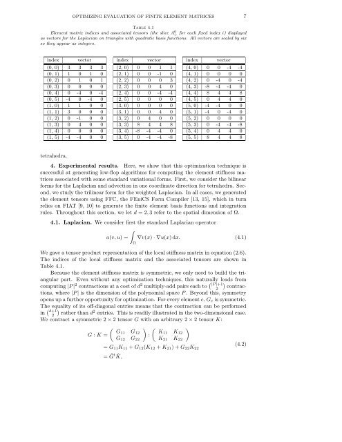
OPTIMIZING <strong>EVALUATION</strong> <strong>OF</strong> FINITE ELEMENT MATRICES 7Table 4.1Element matrix indices and associated tensors (the slice A 0 i· for each fixed index i) displayedas vectors for the Laplacian on triangles with quadratic basis functions. All vectors are scaled by sixso they appear as integers.indexvector(0, 0) 3 3 3 3(0, 1) 1 0 1 0(0, 2) 0 1 0 1(0, 3) 0 0 0 0(0, 4) 0 -4 0 -4(0, 5) -4 0 -4 0(1, 0) 1 1 0 0(1, 1) 3 0 0 0(1, 2) 0 -1 0 0(1, 3) 0 4 0 0(1, 4) 0 0 0 0(1, 5) -4 -4 0 0indexvector(2, 0) 0 0 1 1(2, 1) 0 0 -1 0(2, 2) 0 0 0 3(2, 3) 0 0 4 0(2, 4) 0 0 -4 -4(2, 5) 0 0 0 0(3, 0) 0 0 0 0(3, 1) 0 0 4 0(3, 2) 0 4 0 0(3, 3) 8 4 4 8(3, 4) -8 -4 -4 0(3, 5) 0 -4 -4 -8indexvector(4, 0) 0 0 -4 -4(4, 1) 0 0 0 0(4, 2) 0 -4 0 -4(4, 3) -8 -4 -4 0(4, 4) 8 4 4 8(4, 5) 0 4 4 0(5, 0) -4 -4 0 0(5, 1) -4 0 -4 0(5, 2) 0 0 0 0(5, 3) 0 -4 -4 -8(5, 4) 0 4 4 0(5, 5) 8 4 4 8tetrahedra.4. Experimental results. Here, we show that this optimization technique issuccessful at generating low-flop algorithms for computing the element stiffness matricesassociated with some standard variational forms. First, we consider the bilinearforms for the Laplacian and advection in one coordinate direction for tetrahedra. Second,we study the trilinear form for the weighted Laplacian. In all cases, we generatedthe element tensors using FFC, the FEniCS Form Compiler [13, 15], which in turnrelies on FIAT [9, 10] to generate the finite element basis functions and integrationrules. Throughout this section, we let d = 2, 3 refer to the spatial dimension of Ω.4.1. Laplacian. We consider first the standard Laplacian operator∫a(v, u) = ∇v(x) · ∇u(x) dx. (4.1)ΩWe gave a tensor product representation of the local stiffness matrix in equation (2.6).The indices of the local stiffness matrix and the associated tensors are shown inTable 4.1.Because the element stiffness matrix is symmetric, we only need to build the triangularpart. Even without any optimization techniques, this naturally leads fromcomputing |P | 2 contractions at a cost of d 2 multiply-add pairs each to ( )|P |+12 contractions,where |P | is the dimension of the polynomial space P . Beyond this, symmetryopens up a further opportunity for optimization. For every element e, G e is symmetric.The equality of its off-diagonal entries means that the contraction can be performedin ( )d+12 rather than d 2 entries. This is readily illustrated in the two-dimensional case.We contract a symmetric 2 × 2 tensor G with an arbitrary 2 × 2 tensor K:G : K =( )G11 G 12:G 12 G 22( )K11 K 12K 21 K 22(4.2)= G 11 K 11 + G 12 (K 12 + K 21 ) + G 22 K 22= ˜G t ˆK,
Page 4 and 5: 4 R. C. KIRBY AND A. LOGG AND L. R.
Page 8 and 9: 8 R. C. KIRBY AND A. LOGG AND L. R.
Page 11: OPTIMIZING EVALUATION OF FINITE ELE
Page 14 and 15: 14 R. C. KIRBY AND A. LOGG AND L. R
Page 16 and 17: 16 R. C. KIRBY AND A. LOGG AND L. R

TOPOLOGICAL OPTIMIZATION OF THE EVALUATION ... - BearSpace

You also want an ePaper? Increase the reach of your titles

Delete template?

Save as template?