IMPROVED HUFFMAN CODING USING RECURSIVE SPLITTING ...

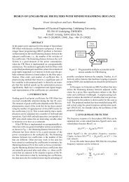
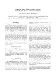
IMPROVED HUFFMAN CODING USING RECURSIVE SPLITTING.Karl Skretting, John Håkon Husøy and Sven Ole AaseHøgskolen i Stavanger, Department of Electrical and Computer EngineeringP. O. Box 2557 Ullandhaug, N-4004 Stavanger, NorwayE-mail: Karl.Skretting@tn.his.noABSTRACTLossless compression of a sequence of symbols is animportant part of data and signal compression. Huffmancoding is lossless, it is also often used in lossycompression as the final step after decomposition andquantization of a signal. In signal compression, thedecomposition/quantization part seldom manages toproduce a sequence of completely independent symbols.Here we present a scheme giving better resultsthan straightforward Huffman coding by utilizing thisfact. We split the original symbol sequence into twosequences in such a way that the symbol statistics are,hopefully, different for the two sequences. IndividualHuffman coding for each of these sequences will reducethe average bit rate. This split is done recursively foreach sub-sequence until the cost associated with thesplit is larger than the gain.Experiments were done on different signals. Theywere decomposed with the Discrete Cosine Transform,quantized, and End Of Block coded, to give the inputsymbol sequence. The results using the split schemewas a bit rate reduction of usually more than 10%compared to straightforward Huffman coding, and 0-15% better than JPEG-like Huffman coding, best atlow bit rates.1. INTRODUCTIONHuffman coding creates variable-length codes, eachrepresented by an integer number of bits. Symbolswith higher probabilities get shorter codewords. Huffmancoding is the best coding scheme possible whencodewords are restricted to integer length, and it isnot too complicated to implement [1]. It is thereforethe entropy-coding scheme of choice in many applications.The Huffman code tables usually need to be includedin the compressed file as side information. Toavoid this one could use a standard table derived forthe relevant class of data, this is an option in theJPEG compression scheme [4]. Another alternative isadaptive Huffman coding as in [3]. While these methodsdo not need side information they use non-optimalcodes and consequently more bits for the symbol codewords.The efficiency of Huffman coding can oftenbe significantly improved by the use of custom madeHuffman code tables. This possibility is also includedin the JPEG compression scheme [4]. The methodsused in this paper all use custom made Huffman codetables.Huffman coding is effective when integer codewordlengths are suitable for the symbol sequence. Generally,this is the case when no symbols have very highprobabilities, especially no symbol should have probabilitygreater than 0.5. If the symbols probabilitiesare 0.5, 0.25, 0.125, 0.0625 or less than 0.05 then ascheme using integer codeword lengths will do quitewell. Huffman codes do not exploit any dependenciesbetween the symbols, so when the symbols arestatistically dependent other methods may be muchbetter.1.1. Lossy signal compressionLossy signal compression often has the following steps1. Decomposition.2. Quantization, often with threshold.3. Run Length and End Of Block coding.4. Huffman coding.Here we compare three different schemes for compression:straightforward, JPEG- like, and recursive Huffmancoding. The two first steps are identical for allthree methods, we use DCT and uniform quantizationwith threshold. The results can then be representedin a matrix where the rows are the frequencies andthe columns are time. The entries are the quantizedvalues, there are as many entries as there are samplesin the signal. The upper left part of this matrix maybe

Block 1 2 3 4 5 6 7 8 · · ·LP (DC) 4 5 5 0 -4 -2 4 2 · · ·BP (AC) 1 0 3 0 0 -1 0 -2 · · ·0 1 1 0 0 4 1 0 · · ·0 0 0 0 5 0 0 -1 · · ·0 0 0 0 0 0 0 0 · · ·HP (AC). ... . ... ... ... ... .. ...· · ·Since we have used a 16 points DCT, the matrix willhave 16 rows (bands) and each block is 16 samples.The three different methods used here all start withthis matrix of quantized values, and use different waysto form the symbol sequences.Straightforward Huffman Coding use only Endof Block coding. The End of Block symbol, (0), andthe rest of the symbols are formed from the quantizedvalues according to this tableValue EOB · · · -2 -1 0 1 2 · · ·Symbol 0 · · · 4 2 1 3 5 · · ·The symbol sequence after EOB coding for the exampleabove will then be:9, 3, 0, 11, 1, 3, 0, 11, 7, 3, 0, 0, 8, 1, 1, 11,0, 4, 2, 9, 0, 9, 1, 3, 0, 5, 4, 1, 2, 0, · · ·.We note that there will be as many EOB symbols asthere are columns in the matrix, and that the symbolsequence will be non-negative integers where thesmaller ones are more probable than the larger ones,because symbols represented by small integers correspondto small magnitude of the quantized values.JPEG-like Huffman Coding makes the symbolsthe same way as JPEG does, each column of the matrixcorrespond to the zigzag scanned sequence of a8 × 8 pixel picture block in JPEG. The DC componentand the AC components are coded separately.The DC component is DPCM coded and the symbolsare defined by the following tableSymbol DPCM difference Additional bits0 0 01 -1, 1 12 -3, -2, 2, 3 23 -7, . . ., -4, 4, . . ., 7 34 -15, . . ., -8, 8, . . ., 15 4..Each symbol is followed by some additional bits touniquely give the DPCM difference. For the data examplethis gives (the two last lines are stored)Quantized DC value 4 5 5 0 -4 . . .DPCM difference 4 1 0 -5 -4 . . .Symbol 3 1 0 3 3 . . .Additional bits 100 1 - 010 011 . . ..For the AC component the zeros are run lengthcoded. Each symbol consists of two parts, the firstpart is the run that tells how many zeros that precedethe value (R), and the second part is the value symbol(S). The value symbols are the same as the symbolsused for the DPCM differences. To completely specifythe value each symbol is succeeded by additional bitsthe same way as for the DPCM differences. The combinedsymbol (represented as one integer) is 16R + S.Symbol (0) is EOB. For the example data this givesQuantized AC value 1 EOB 1 EOB 3 . . .Value symbol (S) 1 0 1 0 2 . . .Preceding zeros (R) 0 0 1 0 0 . . .Symbol (16R+S) 1 0 17 0 2 . . .Additional bits 1 - 1 - 11 . . .Recursive Huffman Coding uses the same symbolsequence as straightforward Huffman coding. Usuallythese symbols are not independent, which meansthat the true entropy (lower limit for possible bit rate)is less than zero-order entropy (lower limit for bit ratefor Huffman code). The proposed scheme takes advantageof some dependencies in the symbol sequenceand exploits this in the Huffman coding procedure.The next two sections of the paper explain the detailsof this method. Note that the method has some limitations.If the symbol sequence is highly correlated, itwill probably be better to try to improve the decompositionpart rather than to hope that this Huffmancoding scheme will utilize all of the correlation. Also,if integer codeword lengths are not suitable then othermethods may be much better.2. SPLITTING THE SYMBOL SEQUENCEThe basic idea is that by splitting a long sequence intoseveral shorter ones in a way that makes the symbolprobabilities (and the optimal code lengths) differentfor each sequence, then individual Huffman coding ofeach sequence will reduce the total number of bitsused for the codewords. On the other hand, therewill be more Huffman code tables to include. Cleversplitting combined with effective coding of the sideinformation should give an improvement in overall bitrate. We choose to use a scheme that first splits thesymbol sequence after End of Block coding into threesequences.2.1. Splitting into three sequencesWhen we examine the End of Block coded sequencewe make the following observations• A symbol succeeding an EOB symbol (0) is theDC component, or possibly another EOB symbol.

• An EOB symbol (0) will never succeed a (1)symbol.This may be exploited by creating three symbol sequencesfrom the original sequence. The first sequencecontains the first symbol and the symbols followinga (0) symbol, the next sequence contains the symbolsfollowing a (1) symbol, and the third sequencecontains all the other symbols. The key to successis that the symbol probabilities will be different forthese sequences. In fact only this splitting improvestraightforward Huffman coding considerably. Usingthis scheme, the example sequence will be split asOriginal EOB sequence: 9, 3, 0, 11, 1, 3, 0, 11, 7, 3, 0,0, 8, 1, 1, 11, 0, 4, 2, 9, 0, 9, 1, 3, 0, 5, 4, 1, 2, 0, . . .First sequence: 9, 11, 11, 0, 8, 4, 9, 5, . . .Second sequence: 3, 1, 11, 3, 2, . . .Third sequence: 3, 0, 1, 0, 7, 3, 0, 1, 0, 2, 9, 0, 1, . . .Then each of these is dealt with independently of eachother and in the same way by the recursive splittingpart of the function.2.2. Recursive splittingThe recursive splitting part either1. splits the input sequence into two sub-sequences,this split is done either(a) by cutting the sequence in the middle or(b) by letting the previous symbol decide towhich sub-sequence the following symbolshould be put into,and then calls itself twice with each of the subsequencesas arguments or2. does Huffman coding of the input sequence, thatis store the Huffman table information and thecodewords into the output bit sequence.The decision rules are: If the symbol sequence is long,1.a is done. Else, we test if splitting (as in 1.b) willreduce the number of bits, and if so, we split as in 1.b,else we do point 2.Cutting in the middle (1.a) is one obvious way tosplit the symbol sequence, especially if the signal isnon-stationary. When sequence length is larger than2 15 , the sequence is split into two sequences of halfthe length. This ensure that no used symbol has aprobability less than 2 −15 . Then the given code wordlengths always will be less or equal to 15, which is themaximum code word length that we allow when wecode the Huffman tables.Splitting by previous symbol (1.b) tries to utilizecorrelation between successive symbols by lettingthe previous symbol decide to which sub-sequence thefollowing symbol should be put into. The first subsequencecontains the symbols following a symbol witha value less or equal than a limit value, the secondsub-sequence contains the other symbols (includingthe first symbol). Using this scheme with limit valueequal 1, one example sequence will be split asEx. sequence: 3, 0, 1, 0, 7, 3, 0, 1, 0, 2, 9, 0, 1, . . .First sequence: 1, 0, 7, 1, 0, 2, 1, . . .Second sequence: 3, 0, 3, 0, 9, 0, . . .By using the median (of the numbers representing thesymbols in the original sequence) as this limit value,we split into two approximately equal size sub- sequences.In addition, the split is done in such a waythat we do not need the decision rule or the limit valueto be included as side information.3. INCREASED SIDE INFORMATIONThe way we have done splitting, very little side informationis needed to specify when and how to split asequence. In fact, we use only one bit to tell whethera sequence is split or not. However, we need to includeas many Huffman tables as we have sequences.To keep this side information small we put a bit of effortinto doing a good job on compact storing of thesetables. This effort pays off; our scheme often uses lessthan one third of the bits to store the Huffman tables,compared to what JPEG uses. Let us start by lookingat how JPEG store the Huffman tables.3.1. JPEG Huffman table specificationUsually this side information is relatively small, andconsequently not much effort has been used in representingthis in few bits. JPEG use a special segment,the DHT marker segment structure, to specify a Huffmantable [4]. In this segment, one byte are used totell how many symbols there are with code length i,for i = 1 : 16, then follows the symbols with one bytefor each. This requires (16 + N) bytes for N symbols.3.2. Efficient Huffman table specificationWe tried several different ad-hoc methods to store theHuffman tables. The problem was to find a methodthat performed well for all possible Huffman tables.We ended up with a method that performed quitewell, which we will now briefly describe. This methoduses 4 bits to give length of first symbol, then for eachof the next symbols a code to tell its length whereSymbol what it means0 same length as previous symbol10 increase length by 11100 reduce length by 11101 increase length by 2111xxxx set symbol length to xxxx

This way of coding the Huffman tables utilize thefact that adjacent symbols often have approximatelythe same probability, and thus approximately the samecodeword lengths.4. SIMULATIONS AND COMPARISONThe three signals used in the compression experimentsare an AR1 (ρ = 0.95) signal, an ECG signal (normalsinus rhythm, MIT100 [2]), and a seismic signal(pre-stack common shot gather [5]). These signalsare very different from each other, the ECG signal isquite regular and the seismic signal is quite noisy. Thesignal length is, 250000 samples, but when we compressedshorter signals, ex. 25000 samples, the graphswere quite similar to the graphs that we include here.All signals were decomposed by the Discrete CosineTransform (block size 16), and then quantized, thequantizing step varied to get signals with differentSignal to Noise Ratios.The three figures show the results for the AR1signal, the ECG signal and the seismic signal respectively.4.1. ConclusionBoth on real world signals and a synthetic signal theproposed Huffman coding scheme does considerablybetter than straightforward Huffman coding, and usuallybetter than JPEG-like Huffman coding, especiallyat low bit rates.5. REFERENCES[1] Allen Gersho and Robert M. Gray.Vector Quantization and Signal Compression.Kluwer Academic Publishers, Boston, 1992.ISBN 0-7923-9181-0Bit rate (in percent of straightforward Huffman coding)110105100959085AR−1 signal (rho=0.95)StraightforwardJPEG−likeRecursive805 10 15 20 25 30Actual SNRFigure 1: AR1 signal compressed at different signalto noise ratios.Bit rate (in percent of straightforward Huffman coding)110105100959085ECG signalStraightforwardJPEG−likeRecursive8010 12 14 16 18 20 22 24 26 28Actual SNRFigure 2: ECG signal compressed at different signalto noise ratios.[2] Massachusetts Institute of Technology.The MIT-BIH Arrhythmia Database CD-ROM,22nd edition, 1992.[3] Mark Nelson, Jean-Loup Gailly.The Data Compression Book. M&T Books, NewYork, USA, 1996. ISBN 1-55851-434-1[4] William B. Pennebaker, Joan L. Mitchell.JPEG: Still Image Data Compression Standard.Van Nostrand Reinhold, New York, USA, 1992.ISBN: 0442012721Bit rate (in percent of straightforward Huffman coding)110105100959085Seismic prestack signalStraightforwardJPEG−likeRecursive[5] Seismic Data Compression Reference Set.http://www.ux.his.no/~karlsk/sdata/805 10 15 20 25 30Actual SNRFigure 3: Seismic signal compressed at different signalto noise ratios.