P Z QS

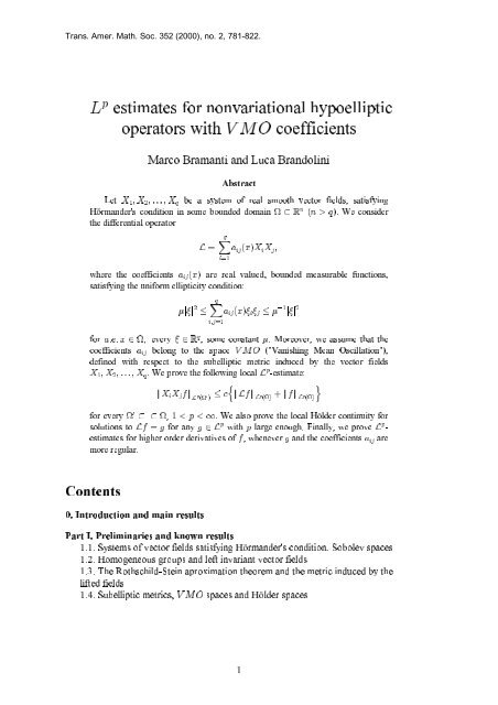
for nonvariational hypoellipticP : estimateswith coefficientsoperatorsw§ §" 34 3 43 4 Ð Ñ Ð Ñ Ð Ñ0 1 + 34I. Preliminaries and known resultsPartSystems of vector fields satisfying Hörmander'os condition. Sobolev spaces1.1.Homogeneous groups and left invariant vector foields1.2.The Rothschild-Stein aproximation theorem and tohe metric induced by the1.3.fields liftedSubelliptic metrics, spaces and Hölder spacesZQS1.4.Trans. Amer. Math. Soc. 352 (2000), no. 2, 781-822.ZQSMarco Bramanti and Luca BrandoliniAbstract" # ;\ß\ßáß\8Letbe a system of real smooth vector fields, satisfyingcondition in some bounded domain ( ). We consider§ 8 € ;Hörmander'sH ‘the differential operator;_ œ34 3 4+ ÐBÑ\ \ ß"3œ"ÐBÑ 34 +where the coefficientsare real valued, bounded measurable functions,satisfying the uniform ellipticity condition:;# c" #.0 00 . 0l l Ÿ + ÐBÑ Ÿ l l3ß4œ";H 0 ‘ .every , some constant . Moreover, we assume that the+Þ/Þ B − ß −forbelong to the space ("Vanishing Mean Oscillation"),+ ZQScoefficients34defined with respect to the subelliptic metric induced by the vector fields:. We prove the following local -estimate:\ß\ßáß\" # ;_: w : :_l š ›l l l ll\\0 Ÿ- 0 b 0_ H _ H _ Hevery , . We also prove the local Hölder continuity for" : _forHH: :to for any with large enough. Finally, we prove -0œ1 1− :solutions_ _ _estimates for higher order derivatives of , whenever and the coefficients aremore regular.Contents0. Introduction and main results1

II. Differential operators and singular integrualsPartDifferential operators and fundamental solutioons2.1.Operators of type j2.2.Some known results about singular integrals in ohomogeneous spaces2.3.III. Representation formulas, properties of Sobolev spaces and localPartestimatesEstimates in Sobolev spaces3.1.Estimates in Hölder spaces3.2." with ‘Therefore, this condition gives a strong regularity property for the differentialspace).. P operatorcondition can be solved, in classical sense, at least for suitable classes ofHörmander'sdomains.of an underlying structure of homogeneous group for which the operator Pexistenceleft-invariant and homogeneous of degree two. Later, in '76, Rothschild and Steinis\ 30. Introduction___________________________________________________________________________________________________________2.4. Proof of Theorem 2.11.0. Introduction and main results_ 8‘, be a system of real vector fields defined in ( ),\ ß\ áß\ G 8 ;b"Let! " ;that is8_ 8`\ œ , ÐBÑ , − G Ð Ñß3 34 34`B4œ"4) and let3œ!ß"ßáß;à 4œ"ß#ßáß8(;\ b\ 3 # !. (0.1)Pœ"3œ"G _that a linear differential operator with coefficients is said to beTRecall__if, whenever the equation is satisfied, in the distributional sense,T? œ 0hypoellipticH H Hsome open set , then implies A famous theorem proved0−G Ð Ñ ?−G Ð ÑÞonby Hörmander in '67 (see 24 ) states that the operator (0.1) is hypoelliptic if and onlyc dif the 's satisfy at every point of the so called "Hörmander's condition": the vector\ 3 H3 3 4 3 4 4 3 3cd, their commutators , the commutators of the 's\ \ ß\ œ \ \ c\ \ \fieldswith their commutators, and so on until a certain step , generate(as a vector= ‘ 8'69 Bony 2 proved that the Dirichlet problem for operators (0.1) satisfyingÒÓInA further problem is that of provinga-prioriestimates, in suitable Sobolev orspaces, for solutions to the equation . For instance, one would like toP? œ 0Hölder: :3 4__a bound on the norm ( ) of in terms of the norms of":_ \\? P?haveandA first result of this kind was achieved in '75 by Folland 17 , assuming the?Þ c dproved a similar result for system of vector fields satisfying Hörmander'sany35c dcondition. This deep generalization was made possible by a technique consisting inlifting the vector fieldsto a higher dimensional space, obtaining new vector fields2

˜3 which are] 3Dirichlet problem for general Hörmander's operators of kind (0.1) is still lacking.thenote that the operators considered in the above papers have always G _Also,a high regularity of the coefficientso.intrinsicallyuseful point of view in the study of these operators, started in '81 with the paperA\ 3are, by definition, the geodesics of the induced metoric. It turns out that the metricfieldsare well shaped to describe geometrical properties related to the operator. Forballscan be naturally employed in the study of hyopoelliptic operators.theoryus turn now to the problem of proving a-priori estimates for classes ofLetmore general than (0.1), and in particular allowing nonsmooth coefficients.operatorsfirst possible extension is that modeled on variatoional elliptic operators:A\ 3\ 3_ # first order \ ? P? ?several results have been proved, including Harnack inequality and existencesetting,size estimates for the Green's function. See also the paper of Franchi-Lu-Wheedenand0. Introduction___________________________________________________________________________________________________________=up to some step , and can be locally approximated by other vectorfree\fieldswhich fit the assumptions of Folland's quoted paper.o: :__Theso that an-estimates proved both in 17 and in 35 areÒ Ó Ò Ó local, theory forcoefficients, in contrast with the fact that-estimates for linear PDEs do not require_ :Ó 16 by Fefferman-Phong. This paper contains the definition of a "subelliptic metric",Òinduced by the vector fields. Roughly speaking, the integral curves of the vectorthe fundamental solution of can be estimated pointwise through the size ofPinstance,metric balls (see Sanchez-Calle, '84, 37 , and Nagel-Stein-Weinger, '85, 33 ).Ò Ó Ò ÓtheseMoreover, these metric balls define a structure of homogeneous space, in the sense of'71, 15 , so that many tools from singular integrals and real-variableÒ ÓCoifman-Weiss,;‡P œ \ + ÐBÑ\" a b3 34 3 (0.2)3ß4œ"denotes the formal adjoint of and the matrix satisfies an ellipticity\ \ + ÐBÑwhere3 ‡ 3 34(in uniform or degenerate sense). For instance, in '92 G. Lu 29 30 studiedÒ ÓßÒ Óconditionoperators of kind (0.2) whereare smooth Hörmander's vector fields, while theÐBÑ 34 +coefficientsare measurable functions satisfying the degenerate ellipticitycondition:;c" # #0 0 0 0- AÐBÑl l Ÿ + ÐBÑ Ÿ -AÐBÑl l"3ß4œ"34 3 4;#0 ‘every , where is an -weight, in the sense of Muckenhoupt, with respect− A Eforto the subelliptic metric induced by the's. In this case the bilinear form;34 3 3+Ð?ß @Ñ œ + ÐBÑ\ ?ÐBÑ \ @ÐBÑ .B b Ð?@AÑÐBÑ .B"( (3ß4œ"allows to give a natural definition of weak solution to the equationand toP? œ 0, prove -estimates for the derivatives in terms of and . In this3Ó 20 , and references therein, for related results. Recently, Franchi-Serapioni-SerraÒ21 have proved that a Harnack inequality for operators of kind (0.2) holdsÒ ÓCassano3

the \ 3 's are Lipschitz continuous vector fields satisfying suitable geometricwhenever(which in particular hold for smooth Höromander's vector fields).assumptions_ œ + ÐBÑ\ \ Ð Ñ_ œ + ÐBÑ\ \ b \ Ð Ñthe other hand, some classes of operators of kind (0.4), modeled onOnoperators, have been studied in '93-'94 by Lanconelli andKolmogorov-Fokker-Planck\ 3aim of this paper is to prove, for operators of type (0.3) these results in theThecase of a system of Hörmander's vector fields, that is without assuming thegeneralstructure of homogeneous group. Explicitly, our main result is theunderlyingfollowing:+ 340. Introduction___________________________________________________________________________________________________________different direction of research is that of studying theanalog ofnon-variationalAoperators (0.1), namely:;34 3 4 0.3"3ß4œ"or;34 3 4 ! 0.4"3ß4œ", again, satisfying some ellipticity condition.+ ÐBÑ with34G #ß!A complete Schauder () theory for operators (0.3) has been obtained in '92 byXu, 40 . Ò ÓC.-J.3 B !3(see 27 , 34 , 28 ): in this case , and has a particular form,Ò Ó Ò Ó Ò Ó \ œ ` \Polidoro! " ;\ß\ßá\which makesa system of Hörmander's vector fields. In these poapers thesolution of the operator is studied, and a Harnack inequality is proved,Pfundamentalthe coefficients constant 28 or Hölder continuous 34 In '96, Bramanti-+ Ò Ó Ò ÓÞassuming34ÒÓ _ :Cerutti-Manfredini 8 proved local-estimates for the same class of operators,the coefficients in the class , with respect to the subelliptic metric.+ Z QSassuming34The classZQS("Vanishing Mean Oscillation", see Sarason 36 ) appeared in thec dof -estimates for non-variational uniformly equations in '91-'93, with_ :ellipticstudypapers of Chiarenza-Frasca-Longo 11 , 12 . Since functions can have someÒ Ó Ò Ó Z QSthekind of discontinuities, this theory extended the classical one, by Agmon-Douglis-_ :1 . The analog theory for parabolic operators with coefficientsÒÓZQSNirenbergdeveloped in '93 by Bramanti-Cerutti 5 . ÒÓwas(see 4 ), the authors proved -estimates for operators of kind (0.4),ÒÓ _ :Recentlywhere the's are a system of smooth Hörmander's vector fields, satisfying Folland'sassumptions of translation invariance and homogeneity, while the coefficientsareZQS, with respect to the subelliptic metric, and satisfyo the ellipticity condition:;# c" #.0 00 . 034 3 4l Ÿ + ÐBÑ Ÿ l l" . (0.5)l3ß4œ"4

_ œ + ÐBÑ\ \\ H l l šl l l l ›_ : Ò Ó0.2. Under the same assumptions of Theorem 0.1, the following estimateTheoremholds#ß: H+ 340. Introduction___________________________________________________________________________________________________________Theorem 0.1. Let;34 3 4"3ß4œ"_, form a system of real vector fields defined in some bounded\ áß\ Gwhere" ;8‘ H( ), satisfying Hörmander's condition (see §1.1 for the§ 8 ;domaindefinition). The coefficientsare real valued bounded measurable functionsÐBÑ 34 +HHin , belonging to the class , defined with respect to the subellipticZ QSÐ Ñdefinedinduced by the vector fields (see §1.4); the matrix (not necessarily\ Ö+ ÐBÑ×metric3 34symmetric) is uniformly elliptic on : ‘ ;;# c" ;#. 0 0 0 . 0 0 ‘ Hkk"kk+ ÐBÑ Ÿ − B −for every , a.e. ,Ÿ34 3 43ß4œ"H Hw.some positive constant . Then, for every , any , there exists: − Ð"ß _Ñ § §forconstant depending on the vector fields , the numbers , the- \ 8ß ;ß :ß Z QSa3 .w34H Hof the coefficients (see §1.4), such that for every belonging to the+ ß ?moduli#ß:space WSobolev§1.1 for definition)Ð Ñ (see#ß:w : :_? Ÿ - ? b ? ÞH _ H _ H\W Ð Ñ Ð Ñ Ð ÑThe above result generalizes the -estimates proved by Rothschild-Stein 35 ,since our operators do not belong to the class considered there, whenever thearenot(in fact, they can be discontinuous). Moreover, we prove the followingG _regularity result:5ß:w :#>5ß:_l l šl l l l ›? Ÿ - ? b ?H H _ H\ \W Ð Ñ W Ð Ñ Ð Ñ5ß_ 5ß:H _ H\ \every positive integer such that and .5 + − W Ð Ñ ? − W Ð Ñfor34From the estimate of Theorem 0.1, we also deduce the local Hölder continuity for_ H:_to the equation , when with large enough, as well as an?œ0 0− Ð Ñ :solutionsextension of this result to higher order derivativeos:\sTheorem 0.3. Under the same assumptions of Theorem 0.1, if0−WsomeÐ Ñfor _ _ H!− Ð"ß _Ñ − Ð Ñ =€ U Uand f for some ( is the "homogeneous dimension":w\will be defined in §1.2), then belongs to some Hölder space (see §1.40 Ð ÑwhichAHfor definition) and5

w < :! Ð Ñ Ð Ñ Ð Ñ\5ß_ H0.4. Under the same assumptions of Theorem 0.1, if + − W Ð Ñß34 \Theorem#ß: 5ß=5ß w 5ß< :! Ð Ñ W Ð Ñ Ð Ñline of the proof of Theorem 0.1 follows, as close as possible, that of theTheresult in 4 , which, in turn, was inspired by 11 5 8 . To explain the mainÒÓ Ò ÓßÒÓßÒÓanalog_ ! ?for which an explicit fundamental solution is known._ ! ,integrals and their commutators can be estimated, respectively, by the classicalsingulartheory, and Coifman-Rochberg-Weiss' theorem on the commutatorCalderón-Zygmundspherical harmonics is also employed, to reduce singular integrals "with variableinto convolution-type singular integrals.kernel"œ0 in a domain is now routine._?now sketch how the above idea can be settled in ouro context.Weto an operator depending also on extra variables; the coefficients are then frozen;˜_ + 34resulting operator can be locally approximated by a left invariant homogeneousthefor which a homogeneous fundamental solution exists. These facts allow usoperator,0. Introduction____________________________________________________________________________________________________________š ›l l l lll0 Ÿ - 0 b 0A H _ H _ Hfor< œ Ð:ß =ÑÞ maxH _ H− W Ð Ñ : − Ð"ß _Ñ − W Ð Ñ 5ßfor some and f for some positive integer some0\=€U, then_š ›l l l lll0 Ÿ - 0 b 0H H _ H\ Afor< œ Ð:ß =ÑÞ maxideas and techniques which are involved, it is worthwhile, as a starting point, tothe steps which form the original idea of Chiarenza-Frasca-Longo 11 , in Ò Ósummarizecase of a nonvariational uniformly elliptic opeorator . _the+ 34 _1. The coefficients of the operator are frozen at some point, getting aconstant coefficient operatorThen any test function?can be represented as a convolution of this fundamentalsolution with .2. From this representation formula another one follows, assigning the secondderivatives of any test function as the sum of two kinds of objects: a singular?orderoperator applied to , and the commutator of this singular integral with the_?integralfor the coefficients , applied to the second order derivatives of .+ ?multiplication343. Next, one takes the norm of each term in the above representation formula;_ :a operator with a function (see 14 ). A standard technique of expansionG^ FQS Ò ÓofThe assumption of coefficients allows "to make small" theZQS4.FQSseminorm of the coefficients. Therefore, the norm of the the commutators can be madesmall, and their contribution taken to the left hand side. So we get a localestimate_ :the derivatives of , in terms of , for any test function whose support is small? ?on_Passing from this result to the local estimate for solution to the equationanyenough.We apply Rothschild-Stein's technique of "litfing and approximation" ( 35 ), as Ò Ó1.well as Folland's results for the homogeneous situation ( 17 ): the operatoris "lifted"Ò Ó _6

commutators of singular integrals.andThe theory of singular integrals and commutators of singular integrals on2.of the fundamental solution corresponding to the frozen operator. Notederivativeswe need a uniform estimate for a family of fundamental solutions depending on athat_ : ?properties of the Sobolev spaces induced by the vector fields, which only in partsomebeen already studied. Finally, from the estimates for the lifted operator _˜,haveplay a minor role in this paper: these are used only in §1.4, to formulate theetc.,assumption on the coefficients in terms of the "natural" metric (instead of theZQSwhich is "natural" for the proof).metrichave a first idea of the proof, the reader who is already familiar with the paperTo0. Introduction___________________________________________________________________________________________________________3 4 \\?to write an "explicit" representation formula forin terms of singular intergals_ :homogeneous spaces is then the natural context whereestimates can be carried out.need the results of Coifman-Weiss 15 , and the extension to homogeneous spacesÒ ÓWeof the commutator theorem for singular and fractional integrals: these results haveproved by Bramanti-Cerutti 6,7 and Bramanti 3 .ÒÓÒÓÒÓbeen3. The expansion of the singular kernels in series of spherical harmonics can berepeated in our context, thanks to an estimatewe have proved in 4 ÒÓthaton thein a possibleway.discontinuousparameter4. The above steps lead to a local estimate on the derivatives of , in terms of, for any test function whose support is small enough. In order to prove, from this? _˜result, the local estimate for any solution to the equationa domain, we need˜_? œ0in _estimates forfollow immediately.the way, we note that the results of 37 , 33 about subelliptic metrics, balls,Ò Ó Ò ÓByRothschild-Stein 35 can give a glance to §§2.1-2.2 and then pass to §3.1, to seeÒ Óofhow the theory of singular integrals on homogeneouso spaces is involved.7

. .?" # ",! ! 3‘ # " ## , but they are not free up to step 2, because dimTrans. Amer. Math. Soc. 352 (2000), no. 2, 781-822.Part I. Preliminaries and known results1.1. Systems of vector fields satisfying Hörmander'os condition.Sobolev spaces_ 8H ‘be real vector fields on a domain ( ). For every\ ßáß\ G § ; Ÿ8Let" ;, with , we defineœÐ áß Ñ "Ÿ Ÿ;multiindex" . 3! ! ! !! ! ! ! !\ œ \ ß \ ßá \ ß\ ácccddd. We call a commutator of the 's of length . We say thatl lœ. \ \ .and8ßáß\ =B −satisfy Hörmander's condition of step at some point if\" ; !‘8Ö\ B ×spans .! !a b! ± ±Ÿ=‘be the free Lie algebra of step on generators, that is the quotient of=ß; = ;LetZabthe free Lie algebra with;generators by the ideal generated by the commutators ofat least . We say that the vector fields , which satisfy the=b"\ ßáß\length" ;8‘condition of step at some point , are free up to order at if= B − =BHörmander's! !Zab=ß; Ÿdim , as a vector space (note that inequality always holds).8œConsider vector defining Lie of Heisenberg groupExamples. the fields $ the algebra thein : ‘` ` ` ``œc œc%X\ß] B c ]œ b#C \œcd; 2 ; 4`B `> `C `> `>Þ ‘ $ÐBß Cß >Ñ −forWith the above notation, we would write:kk k k a bkkœ\ \ œ] \ œ c%X " œ" œ" " œ; ; ; ; 2 ; 2, 2.\" # Ð#ß"Ñ$\ , satisfy Hörmander's condition of step 2 at every point of , and they are free\" #‘Zabto step , because dim .# $ œ #ß#upOn the other hand, if we consider" #``œ \ œ B ; ;\`B`C, then , satisfy Hörmander's condition of step 2 at every point ofÐBß CÑ − \ \for# #ß#Þ‘ Za b Theorem 1.1. (Lifting Theorem, Rothschild-Stein, see [35] p. 272). Let \ ßáß\" ;_ 8H ‘real vector fields on a domain satisfying Hörmander's condition ofG §be8b" RH !at some point . Then in terms of new variables, , , there exist=B − > áß>stepfunctions ( , ) defined in a neighborhood ˜- 36 ÐBß>Ñ "Ÿ3Ÿ; 8b"Ÿ6ŸR YsmoothRc8˜˜ab0 H ‘ H! ! 3such that the vector fields given byœ B ß! − ‚ œ \of8

5ß: 8 : 85ß: 8 :definitions can be given for function spaces defined on a bounded domainAnalogousAlso, we can define as usual the spaces of functions vanishing at the boundary,H.‘ R RÐ;ß=Ñ. .?" # ",! !−E a b‘ R e.g.I. Preliminaries... §1.1. Systems of vector fields satisfying Hörmander's condition...___________________________________________________________________________________________________________R`˜œ\ b ÐBß>Ñ 3œ"ßáß;3 3 36\" -6œ8b"`>6Hörmander's condition of step and are free up to step at every point in . ˜= = YsatisfyIn this paper we will use several kinds of Sobolev spaoces:81.2. If is any system of smooth vector fields in ,^ œÐ^ ß^ ßáß^ ÑDefinition" # ;‘can define the Sobolev spaces of -functions with derivatives, withW 5we^‘ _:to the vector fields 's, in ( , positive integer). Explicitly,^ "Ÿ:Ÿ_ 5respect3ab_5;" # 2 : 8ll l l""ll0 œ 0 b ^ ^ á^ 0 Þb ‘ _ ‘ _ ‘a4 4 4 Ð ÑW Ð Ñ^2œ"4œ"35ß:WÐ Ñ!^,H .5ß: 5ß:In particular, we will denote byW ß W, the Sobolev spaces generated,\\˜abrespectively, by the original vector fields\ ßáß\and the lifted ones" ;ˆ ‰\ ßáß\˜ ." ;˜1.2. Homogeneous groups and left invariant vector fnields, are generators of the free Lie algebra and/ áß/ ;ß=" ; Za bIf! ! ! ! !cccddd/ œ / ß / ßá / ß/ áthere exists a set of multiindices so that is a basis of as aE Ö/ × ;ß=then! ZRZ ‘space. This allows us to identify with . Note that Card while;ß=E œ Rvectormaxl lœ=, the step of the Lie algebra.ab!−E!The Campbell-Hausdorff series defines a multiplication in (see [37]):"! ! ! ! ! ! ! ! ! ! !? / ‰ @ / œ ? b@ / b ? / ß @ / bá#: ; : ; – —" " " "a b"! ! ! ! !−E−E−E−E−Ethat makes the group , that is the simply connected Lie group associated tooZab;ß=. We can naturally define dilations in by RÐ;ß=Ñ!± ±!−E−E . (1.1)HÐ Ñ ? œ ?- -! !Ša b ‹ ˆ ‰!are automorphisms of , which is therefore a homogeneous group, in theRÐ;ß=ÑTheseof Stein (see [38], p. 618-622). We will call it , when the numbers areK;ß=senseunderstood. (Actually, throughout the paper the numbers are fixed once;ß=implicitlyand for all).9

above definition of norm is taken from [18]. This norm is equivalent to thatThein [38], but in addition satisfies (1.2. ), a property we shall use in the proof of,defined2.11 (to expand a kernel in series of spherical harmonics). The propertiesTheorem--) are immediate while (1.2. ) is proved in [38], p.620 and (1.2. ) is Lemma+,- . /(1.2.‘ R K! R".Ð@?ÑŸ.Ð?ß@ÑŸ-.Ð@?Ñ Ð ,Ñ, , ; 1.3.-k k kFÐ?ß

`? "kk kkO ,$ "! !I. Preliminaries... §1.2 Homogeneous groups and left invariant vector fields___________________________________________________________________________________________________________we define the convolution of two functions in as KNext,c" c"( (‘RR‘œ 0ÐB ‰ C Ñ 1ÐCÑ .C œ 1ÐC ‰ BÑ 0ÐCÑ .C,Ð0‡1ÑÐBÑfor every couple of functions for which the above iontegrals make sense.7 7? ?Letbe the left translation operator acting on functions:Ð0ÑÐ@Ñ œ 0Ð? ‰ @ÑÞsay that a differential operator on is left invariant if forT K TÐ 0Ñ œ ÐT0ÑWe7 7? ?smooth function . From the above definition of convolution we read that if is0 Teveryany left invariant differential operator,TÐ0‡1Ñ œ 0‡T1(provided the integrals converge).$say that a differential operator on is homogeneous of degree ifT K € !We$T 0 HÐ Ñ? œ ÐT 0ÑÐHÐ Ñ?ÑŠ a b‹- - -- ‘ Revery test function , , . Also, we say that a function is0 € ! ? − 0for$ ‘homogeneous of degree−if$R- - - ‘Ñ?Ñœ 0Ð?Ñ €! ?−for every , .0ÐHÐif is a differential operator homogeneous of degree and is aT 0Clearly,$ $ $function of degree , then is homogeneous of degree . ForT0chomogeneous# # "!`" !is homogeneous of degree .? cexample,4by ( ) the left-invariant vector field on which agrees with] 4œ"ßáß; KDenote`4. Then is homogeneous of degree and, for every multiindex , is! ] " ]at`? 4of degree | |. !homogeneous1.3. The Rothschild-Stein approximation theorem andn the metricinduced by the lifted fields1.3. A differential operator on is said to have local degree less than orKDefinitionto if, after taking the Taylor expansion at of its coefficients, each termj !equalis homogeneous of degree . ŸjobtainedRemark 1.4. It is useful to make more explicit the above definition, in the case ofG _fields, that is first order differential operators. If is a -function, not0Ð?Ñvectoranalytic, we can write, for every fixed integer , its Taylor expansion forOnecessarily?Ä!:5ON0Ð?Ñ œ - : Ð?Ñ b 9 ?54 54ˆ ‰ kk""5œ!4œ"O_the error term is a -function, the 's are constants and9l?l G -where54ab11

N 5denote all the monomials of degree (in the usual sense). Now, any isalgebra).for any integer we can also rewrite the Taylor expansion of withO 0Therefore,ll Oll O``?O ,`? !! states that we can locally approximate these vector fields with the left invariantSteinfields , defined at the end of §1.2.] 3vectornow state Rothschild-Stein's approximation Theorem (see [35], p. 273). OurWeis taken from [37], p. 146.formulationis a diffeomorphism onto the image, for every ;@ 00 ±Z −Za)0 a bI. Preliminaries... §1.3. The Rothschild-Stein approximation theorem and the metric...___________________________________________________________________________________________________________54 54: 5 :4œ"š ›! !54 54homogeneous of degree , with ( being the step of the Lie5Ÿ Ÿ5==alsorespect to the homogeneity, at the following way:5ONœ - : Ð?Ñ b 9 ?˜ ˜0Ð?ш ‰ ll""54 545œ!4œ"_ˆ ‰54 54the error term is a -function, the 's are constants and the 's˜˜9 ? G - :wherehomogeneous monomials of degree . Let now 5areTœ"-Ð?Ñ!!!−Ebe a vector field of local degreethis means that we can write, for every integerŸj: O,5ON!54 54``T œ - : Ð?Ñ b 1Ð?Ñ" " ": ;! !!−E 5œ!4œ"`? `?_, , the 's are constants, the 's are1Ð?Ñœ9 ? 1−G - : Ð?Ñwhereˆ ‰!54 54`monomials of degree and every term appearing in the5 : Ð?Ñhomogeneous54is a differential operator homogeneous ofo degree , .Ÿ j 3Þ/Þ c 5 Ÿ jexpansionkk˜˜, be the vector fields constructed in Theorem 1.1, and let\ áß\Let" ;R0 ‘ 0−EÐ Ñ× − Ybe a basis for for every . A remarkable result by Rothschild-Ö\˜˜! !˜0 (Forßdefine the map− Y, ( 0 ! ! Ð ÑœÐ? Ñ −E@with‹ " Š˜! !( 0? \exp .œ!−E˜˜Theorem 1.5. Let\ ßáß\be as in Theorem 1.1. Then there exist open" ;Rof and of in , with such that:Y ! Z ß[ [ § § Zneighborhoods0 ‘!@ 0for every ;0ÐZѪY −[b)R_@ ‘ @ 0 ( @ (, defined by is ;ÀZ ‚Z Ä Ð ß Ñœ Ð Ñ G Z ‚Zc)12

! a bMore generally, for every we can write! −Ee)@ 00 0œ bV˜ 0! ! !] \!kkmeasure.Lebesguewill compute the Jacobian determinant of the inverse mappingWeI. Preliminaries... §1.3. The Rothschild-Stein approximation theorem and the metric...___________________________________________________________________________________________________________In the coordinates given by , we can write on , where is\ œ ] bV Y Vd)3 3 3 3˜vector field of local degree depending smoothly on . Explicitly, thisŸ! −[a0_that for every :0−G Kmeans00 0\ 0Ð † Ñ œ ] 0 bV 0 Þ Ð Ñ3 3 3a b ‹a b Š ‹a b abŠ1.5@ ( @ (˜0a vector field of local degree depending smoothly on .V Ÿ c"with! 0Other important properties of the mapare stated in the next theorem@:Rothschild-Stein, see [35], pp. 284-7)(1.6. Let be as in Theorem 1.5. For , defineZ ß − Z 0 (Theorem@0( a b l lß œ Ð ß Ñ ,30(where† llis the homogeneous norm defined above. Then:c";Ðß Ñœ Ðß Ñ œc Ðß Ña)@0( @(0 @(0whenever and are both ,30( 30'Ðß Ñ Ðß Ñ Ÿ"b)b1)"Î="c"Î=l l Š a b ‹@0( @' ( 30' 30' 30(Ðß Ñc Ðß Ñ Ÿ- ß b Ðß Ñ Ðß Ñis the step of the Lie algebra;= whereb2Ñ( 30' 3(0a b Š a b a b‹ß Ÿ - ß b ß .3'@ (0Under the change of coordinates , the measure element becomes:?œ Ð Ñc)ab0 a b ll ,(. œ-Рц "bS ? .?is a smooth function, bounded and bounded away from zero in . The-Ð Ñ Zwhere0@ 0(is true for the change of coordinates . ?œ Ð ÑsameProof of c). Observe that this point is not exactly the same stated in [35]: in fact, theya particular measure , in order to have . For us always denotes the. - ´ " .choose( (c"0( @œTo Ð?Ñ. do this, set13

position.the square matrixDefining! !( a) andc"I. Preliminaries... §1.3. The Rothschild-Stein approximation theorem and the metric...___________________________________________________________________________________________________________Rfor every( !˜! !`5\ œ - Ð Ñ − E`("5œ"5and rewrite the left hand side of (1.5) as`0`! 0 0( @ ( @ (- Ð Ñ." a b ’ “ab a b ab"54`? `4 5 (45Then (1.5), evaluated atbecomes:( 0 œ ,`0`00 ! !!!40 @ (" ab ’ “ a ba b ab ˆ ‰"5( 0(œÐ Ñ ! œ ] 0 b V 0 Ð!Ñ œ ] 0 Ð!Ñ.-`? `4 4 55| | , changing for a moment our notation we can assume thoat the multiindexEœRSinceR 0Ð?Ñœ? 2 œ"ßáßRis actually an index ranging from 1 to . Choosing ( ),2!`! 0 ! !2 œ- Ð Ñ œ ] ? ! œ( 0c d c da ba b ab"2 20 @ ( $5`(55where the last equality follows recalling that.! !0 ! œ 0 >] exp]cdab a bÎ>œ!.>that exp equals, in local coordinates, with in the -th>] Ð!ßáß>ßáß!Ñ >andÑ œ - Ð Ñ0 0GÐ5!š ›!50 @ ( ( 00letting be the Jacobian determinant of the mapping at weNÐ Ñ ? œ Ð Ð ÑÑ œandget0 0cd.GÐ Ñ †NÐ Ñœ"Detc"0( @the Jacobian determinant of the mapping at equalsœ Ð?Ñ ? œ !Hence. Since the determinant of is a smooth function in , itGÐ Ñ ´ -Ð Ñ œ Ð?Ñ ?Detcd0 0 ( @ c"0equals-Рц "bS ?ll .0 a bab@ 0analog result for the change of coordinates follows point ( the?œ Ð ÑTheof the map in .?È? KsmoothnessWe now need the following1.7. (Homogeneous space, see Coifman-Weiss, [15]). Let be a set andWDefinition‚ W Ä ! _Ñ . +[ , . We say that is a quasidistance if it satisfies properties (1.3. ),.ÀW14

), (1.3. ). The balls defined by induce a topology in ; we assume that the balls, - . W(1.3.open sets, in this topology. Moreover, we assume there exists a regular Borelare. \will use still hold under these more general assuomptions.we1.6 implies the followingTheorem0 −W3 0 boundedis a homogeneous space.3 0 ˜sup ( 0I. Preliminaries... §1.3. The Rothschild-Stein approximation theorem and the metric...___________________________________________________________________________________________________________measure on , such that the "doubling condition" is satisfied:F ÐBÑ Ÿ - †F ÐBÑ.#<

\˜,. \domain of , is a homogeneous space, and we want to study‘ 8 \bounded. \˜. \˜vector fields in . The there exist constants such that‘ R !lifted\˜‘˜\˜I. Preliminaries... §1.4. Subelliptic metrics, VMO spaces and Hölder spaces___________________________________________________________________________________________________________Lemma 1.11. (Sanchez-Calle, see [37], Lemma 7 p. 153). With the above notation,˜Ð ß ÑŸ. Ð ß ÑŸG Ð Ñ ß −Wfor every .-30( 0( 30( 0(important property proved for these subelliptic metrics is that, whenever is \Thea system of Hörmander's vector fields,is locally doubling, with respect to theLebesgue measure (see [16], or Lemma 5 p. 151 in [37]). In particular, ifWis anyÐWß. ß.BÑrelationship between the space defined over this homogeneous space, andZQSthespace that we have already introduced. Now, quoting Soanchez-Calle,ZQS theproblem is that there is no clear relation between and . In. ."The\ \˜particular, a ball fordoes not look, in general, like the product of a balland some ball in -space. However, and this is the key. ÐR c8Ñfor\point, the volume of a ball foris, essentially, the volume of the ball ofsame radius for , times the volume of some ball in -space".. ÐR c8Ñthe\(See [37], p.144).Theorem 1.12. (Sanchez-Calle, see [37], Theorem 4 p. 151 and Lemma 7 p. 153).8‘˜( ) be smooth Hörmander's vector fields in , and be their\ 3œ"ßáß; \Let3 38 < ß-ßG €!"volaa abbbF Bß2 ß< ŸGw Rc8 w\\F Bß < † 2 − À Dß 2 − F Bß 2 ß < ŸvolvolŸb a b a ba b a b˜aaa abbbF Bß2 ß< Ð Ñvol 1.7ŸGevery and . (Here "vol" stands for the Lebesgue measure inD − F ÐBß -

˜˜F ÐBß>Ñß< # #‘˜\ ab\˜ 0 3 0 ! − Ð!ß "Ñ 5‘ 8 ^! Ð ÑBßC−BÁC! !˜5ß! abI. Preliminaries... §1.4. Subelliptic metrics, VMO spaces and Hölder spaces___________________________________________________________________________________________________________By (1.6) we have (with a constant to be chosen later):-Proof.˜˜cl0ÐCß =Ñ c 0 l .C .= Ÿ l0ÐCÑ c -l .C .= Ÿc( (\ab\ \F ÐBß>Ñß< F ÐBß>ÑßÑß < 0ÐCÑ c - .C Ÿvolœ\ F BßÑß

now define various differential operators that we will handle in the following. FirstWeall, our main interest is to studyof_ œ + ÐBÑ\ \34 ! 3 4!3ß4œ"! −we will consider the approximating operator,˜_ ! ,following Proposition, proved in [4], summarizes some properties of theseTheoperators.\ 3_ abII. Differential operators and singular integrals. §2.1. Differential operators...___________________________________________________________________________________________________________Part II. Differential operators and singular integfrals2.1. Differential operators and fundamental solutionns;34 3 4,"3ß4œ"the 's are smooth real vector fields satisfying Hörmander's condition of step\ =where3834H ‘some domain , and the matrix satisfies (0.5). Applying Theorem 1.1§ + ÐBÑinthese fields, we obtain the vector fields which are free up to order and satisfy\ =to3˜RH ‘ 0 H˜˜condition of step , in some domain . For , set=§ œ ÐBß >Ñ −Hörmander's34 34ÐB>Ñœ+ ÐBј , and let+;0˜ ˜ ˜34 3 4_œ + Ð Ñ\ \ ˜"3ß4œ"˜ ˜H _ 0 H˜be the lifted operator, defined in . Next, we freeze at some point , andconsider the frozen lifted operator:;.œ + Ð Ñ\ \ ˜0˜ ˜ ˜_"In view of Theorem 1.5, to studyon the group : Kdefined;‡+ Ð Ñ] ] " ˜ .œ_ 0!34 ! 3 43ß4œ"Proposition 2.1. Letbe smooth vector fields satisfying Hörmander's condition of8 ;34in some domain , and let the matrix be uniformly elliptic on .=§ + ÐBÑstepH ‘ ‘Then:H_+ ÐBÑ Gif the coefficients are , then can be rewritten in the formÐ3Ñ34;_ œ ^ b ^5 # !"5œ"the vector fields are linear functions of the 's and their commutators of^ \where5 32; therefore the 's satisfy Hörmander's condition of step , is^ length b" =5 _:in and the local estimates for follow from [35].H _ _hypoelliptic19

_ ‡ !> a bsecond result is due to Folland-Stein (see Proposition 8.5 in [19], PropositionThein [17]):1.82cU 2 !2U X 22 2 a bProposition 2.1, the operator satisfies the assumptions of Theorem 2.2;_ ‡ !Byit has a fundamental solution with pole at the origin which is homogeneoustherefore,>0 !II. Differential operators and singular integrals. §2.1. Differential operators...___________________________________________________________________________________________________________‡!!Ð33ÑFor every , the operator is hypoelliptic, left invariant and−˜0 H _RXof degree two with respect to the structure of homogeneous group in Khomogeneous; moreover, the transpose of is hypoelliptic, too.‘ _ _We will apply tothe results contained in the following two theorems. The firstis due to Folland (see Theorem 2.1 and Corollary 2.8 ion [17]):_Theorem 2.2. Existence of a homogeneous fundamental solution. Letbe a leftinvariant differential operator homogeneous of degree two on a homogeneous group__ XU, such that and are both hypoelliptic. Moreover, assume 3. Then there isKa unique fundamental solutionsuch that:>_RÐ+Ñ − G Ï ! à> ‘aefbÐ,Ñis homogeneous of degree# c U àfor every distribution 7Ð-Ñß> _7 > 7Ð ‡ Ñ œ ‡ œ a b ._7Note that the only possibility in order the conditionU $not to hold is" #\ ß\; in this case the Lie algebra generated by is abelian, and thisUœRœ8œ#_ _ :means thatis a uniformly elliptic operator in two variables, for which a completetheory is known to hold, whenever the coefficients are bounded (see Talenti, 39 ).+ 34 c d_RTheorem 2.3. Let be a kernel which is and homogeneous ofO G Ï !aefb2‘abdegree , for some integer with ; let be the operator2 2X0œ0‡Oa left invariant differential operator homogenevous of degree . ThenT 22beand let2 22 2X 0 œ 0‡T O b 0P.V.Š ‹ !T2 2 _ Ref! ‘some constant depending on and . The function is ,T O T O G Ï !forof degree and satisfies the vanishing property:cUhomogeneous2T O ÐBÑ.B œ !!

‘ R > 0 _ ! 0 _! cdsupl lWe also need some uniform bound for0 ! .any . Moreover, for the 's appearing in (1.9), the uniform bound3ß4œ"ßáß; ! 34for# #a bII. Differential operators and singular integrals. §2.1. Differential operators...___________________________________________________________________________________________________________34 !coefficients . Also, set for ,˜+ Ð Ñ 3ß4œ"ßáß;frozen034 ! 3 4 !Ð à?Ñœ]] Ð à†ÑÐ?Ñc d .> 0 > 0a b a b>0 > 0! 34 !theorem summarizes the properties of and ; that we willà† †Nextneed in the following. All of them follow from Theoreoms 2.2-2.3.R0 ‘−!Theorem 2.4. For every :_R>0 ‘!† − G Ï ! à, Ð+Ñb a b efa† Ð# c UÑà, is homogeneous of degreeÐ,Ñ>0!‘ R0 @ −for every test function and every ,Ð-Ñab‡ c" ‡_ > 0 > 0 _!! !!0Ð@Ñ œ 0 ‡ à † Ð@Ñ œ à ? ‰ @ 0Ð?Ñ .?àŠ a b‹ ( ˆ ‰‘ Rfor every , there exist constants such that3ß4œ"ßáß; Ð Ñmoreover,! 034 !c" ‡ ‡3 4 34 ! 34 !! ! (1.9)] ] 0Ð@Ñ œ T ÞZ Þ à ? ‰ @ 0Ð?Ñ.? b Ð Ñ † 0Ð@Ñà( ˆ ‰_R> 0 ‘34 !Ð.Ñ à † − G Ï ! à0 34 ! >b a b efaabà † cUis homogeneous of degree ;Ð/ÑÐ0Ñ34 ! 34 !> 0 > 0 5every .à? .?œ à? . Ð?Ñœ! V€

in §2.1, which will induce singular and fractional integrals on theintroducedspace described in Proposition 1.8. Here we follow Rothschild-SteinhomogeneousApproximation Theorem (Theorem 1.5) and the definition of differential operatorthelocal degree , and taking into account the dependence on the frozeno point :Ÿj 0 !ofLc da b c da b"jcU H !˜_ !II. Differential operators and singular integrals. §2.2. Operators of type j___________________________________________________________________________________________________________2.2. Operators of type jWe are going to define suitable kernels, adapted to the operatorthat we haveÓ Ð à †Ñ35 , with slight changes to handle the frozen variable . Let be as in §2.1,Ò0 > 0! !and let! !0 0( 0>0 @(0 (!ab5 Ð à ß Ñ œ +Ð Ñ Ð à ß Ñ,Ð Ñbe the Rothschild-Stein-like parametrix (see [35], p.297) where+ß ,are cutofffunctions fixed once and for all. Roughly speaking, a singular kernel is a function with< ‘the same properties asLet us compute these derivatives using\\ 5Ð à†ß ÑÐÑ. 4 ! ! 0 ( 03˜˜cabd,>0 @( ( 0˜\ +Ð†Ñ Ð à † ,Ð ÑÐ Ñœ3 !, ,3 ! 3 !0 > 0 @ (0 ( 0 ( > 0 @ (0˜d c da ba b a bcœ \ +Ð Ñ Ð à Ñ,Ð Ñ b +Ð Ñ,Ð Ñ ] Ð à † Ñ b(da b a bc3 !b+Ð Ñ,Ð ÑV Ð à †Ñ, .0 ( >0 @(0third term can be expanded, for every positive ionteger OThe, (see Remark 1.4) as5ON!` Ð à †Ñ>0+Ð Ñ,Ð Ñ - : Ð † Ñ ß b0 ( ( @ ( 0!" " J ab a bŒ 9 a b"3 54 54!!−E 5œ!4œ"`?>0!@ ( 0 ,(! !b- Ð Ñ 1 ІÑ` Ð à †Ñ3 39a b aŒb Ÿ`?!O_! ! !‰ ll ˆab, , , are homogeneous1 Ð?Ñ œ 9 ? - Ð Ñ - − G : Ð?Ñwhere3 3 54 54( (3kkof degree and for every , appearing in the sum.5 5 5monomials! !The above computation motivates the followingDefinition 2.6. We say that is a frozen kernel of type , for some5Ð à ß Ñ j0 0 (!integer , if for every positive integer we can writej 7nonnegative70 0( 0 ( >0 @(0 0 ( >0 @(0! 3 3 3 ! ! ! ! !5Ð à ß Ñ œ + Ð Ñ, Ð Ñ H Ð à †Ñ Ð ß Ñ b+ Ð Ñ, Ð Ñ H Ð à †Ñ Ð ß Ñ3œ"3 3 7 3, ( ) are test functions, are differential operators such+ , 3œ!ß"ßáL Hwherefor , is homogeneous of degree (so that is3œ"ßáßL H Ÿ#cj H Ð à †Ñthat:3 3 ! >07a homogeneous function of degree ), and is a differential operator suchhas derivatives with respect to the vector fields ( ).H Ð à †Ñ 7 ] 3œ"ßáß;that! 3>0 !say that is a frozen operator of type if is a frozen kernelXÐ Ñ j " 5Ð à ß ÑWe0 0 0 (! !type and j of22

0 0 ( is a variable kernel of type , andfrozen kernels of type 2, 1. We point out explicitly these examplesrespectively,we will use them several times in the followiong.becauseFor this follows from the previous Lemma. For we have to showj # jœ"Proof.the differentiation of the integral can be carroied out.how0 !5 Ð à ß Ñœ+ ] à ß ,solution with its regularized version :> > &II. Differential operators and singular integrals. §2.2. Operators of type j___________________________________________________________________________________________________________0 0 0 0 ( ( (Ñ0Ð Ñ œ 5Ð à ß Ñ0Ð Ñ.( ;XÐ! !! !say that is a frozen operator of type if is a frozen kernel of typeXÐ Ñ ! 5Ð à ß Ñwe0 0 0 (! and0 0 0 0 ( ( ( ! 0 0 0X Ð Ñ0Ð Ñ œ T ÞZ Þ 5Ð à ß Ñ 0Ð Ñ . b ß 0 ß( a b a b! ! !!! 0 0 (is a bounded function. If is a frozen kernel of type , we say that5Ð à ß Ñ jwhere5Ð à ß Ñj0 0 0 ( ( (X0ÐÑœ5Ðà ß Ñ0ÐÑ.(a variable operator of type (if , the integral must be taken in principal valuej jœ!issense and the termß 0must be added).!00 0ab a b‡ c"2.7. Note that, since is selfadjoint, . Recalling alsoÐ à?Ñ œ Ð à? ÑRemark_ > 0 > 0! ! !c"@0( @(0 0 0(, we easily see that if is a frozen kernel of typeÐß Ñœ Ðß Ñ 5Ð à ß Ñ jthat!!also is a frozen kernel of type .5Ð à ß Ñ jthen0 ( 0The computation carried out before Definition 2.6 esosentially proves the followingˆ ‰ ab5Ð à ß Ñ j " \5 Ð à†ß Ñ2.8. If is a frozen kernel of type , then is˜0 0 ( 0 ( 0Lemma! 3 !frozen kernel of type . jc"a0 0( 0 >0 @(0 ( 0 ( 0˜instance, if , , then , ,5 Ð à ß Ñ œ +Ð Ñ Ð à Ñ,Ð Ñ 5 \ 5 à † ßFora b a ba b! ! ! ! 3 ! !\ \ 5 à †ß 3ß4œ"ßáß;˜ (for ) are, respectively, frozen kernels of type 2, 1,3 4 ! ! 0 ( 0˜aba b0.( (, are,+Ð Ñ,Ð Ñ V Ð à † Ñ ß +Ð Ñ,Ð Ñ ] V Ð à † Ñ ßMoreover,0 ( >0 @(0 0 ( >0 @(0da b c da ba b a bc3! 4 !3! 3 !XÐ Ñ j " \XÐ Ñ2.9. If is a frozen operator of type , then is a frozen˜0 0Lemmaof type . jc"operatorview of the result for we can assume, without loss of generality, that thej #Inof XÐkernelof the kindÑ be0 0( 0 >0 @(0 (a b ." ! 4 !ab a bab" "ß&introduce a regularized version of , say , defined replacing the fundamental5 5We23

&Ð ß ?Ñ œ ß HÐ ? Ñ? Þ˜3 " !the dots stand for nonsingular terms; now changing variable and denoting withwhere? 0a b the jacobian determinant we getN4 ! 3 X c"4 ! 3 X c"0 0 ( ( ( 0 > 0 @ 0 0] 30 deeper property relating frozen operators of type with differentiation by is ˜j \ 3AII. Differential operators and singular integrals. §2.2. Operators of type j___________________________________________________________________________________________________________"c"‰ ll ˆ> 0 > 0! !Uc#%? bll abThen, in distributional sense,0 0 ( ( (\ 5 à ß 0 . œ•( a b a b”3 "ß !˜ 0 ( 0 ( (&•( a ba b a ba b”\ 5 à †ß 0 . œlim œ&Ä!&•( ab a babab a b”+ ] ] à ß , 0 . bálim œ&4 !0 > 0 @ ( 0 ( ( (3Ä!c"&0 > 0 @+ ] ] à? ,0 ? N ? .?bá œlim œˆ ‰3 4 !0 0&Ä!•( ab a ba b ab ab”&‰ ˆ ‰ ˆ+ ] à? ] ,0 ? N ? .?bá œlim œ&0 > 0 @0 0Ä!•( ab a b a b ab ab”0 > 0 @0 0œ + ] à? ] ,0 ? N ? .?bá Þ•( ab a b a b ab ab”‰ ˆ ‰ ˆTherefore˜3 " ! 4 ! 3X c"‰ ˆ ‰ ˆ\ 5 à ß 0 . œ + ] à † ß] ,0 † N † bá•( a bab ab a b a b ab ab¡”The last expression is the distributional derivativeof a the homogeneous distribution>0aà † b. By Theorem 2.3, this equals]4 !c"0 0 0TÞZÞ + ] ] à? ,0 ? N ? .?b ,0 N ! bá œab a ba b ab ab a ba bab abˆ ‰(> 0 @ ! 0 03 4 ! !0ab a ba bab a baba b(0 > 0 @ 0 ( ( ( ! 0 0 03 4 ! !œ T ÞZ Þ + ] ] à ß ,0 . b ß 0 b áwhere the dots stand for a frozen operator of type one, applied to ,a bis bounded0 !0!! ! !a b a ba ba b a bTheorem 2.3, and therefore is bounded in .ß œ ,0 N ! ßby!0 0 !0 0 00contained in the following:24

! 5 ! 5 ! !35œ"above property is analogous to property (14.8) in [35], aond can be proved withThesame computation.the% .that denotes the modulus of , defined in §1.4).( + ZQS +(Recallto apply several results about integral operators on homogeneous spaces, whichneedrecall here in a form which is suitable for our pourposes.wesatisfying:kernel- BßC−Wthe growth condition: there exists a constant such that, for every ,3ÑII. Differential operators and singular integrals. §2.2. Operators of type j___________________________________________________________________________________________________________2.10. If is a frozen operator of type , thenXÐ Ñ j !Theorem! 0;X \ bXÑœ \XÐ0 0 0˜˜" a b a ba b0suitable frozen operators of type ( ).Xj 5 œ!ß"ßáß;for5 !The following sections of this part will be devoted oto prove:a variable operator of type . Then for everyX ! : − Ð"ß _ÑbeTheorem 2.11. Letexistssuch that:- œ -Ð:ß XÑthereÐ3Ñ:l l l lŸ - 0 0 −for everyX0: :_Ð33Ñ:l l l l l lŸ- + 0 0 − +−FQSfor every , .XÐ+0Ñc+†X0: ‡ :_% ( %++ − Z QS € ! < œ

, , set0 − : − Ð"ß _Ñ_ : For0ÐBÑ œ 5ÐBß CÑ 0ÐCÑ . ÐCÑO% _ %" " # $ .estimate (2.13) has been proved in [6], and the estimate (2.12) is aTheof results in [15] and [13] (see [6] for detaiols).consequencea b a b !c" for some .II. Differential operators and singular integrals. §2.3. Homogeneous spaces...___________________________________________________________________________________________________________- € ! € ! Q € "the mean value inequality: there exist constants , , such33Ñ# "! < ! Q< !for every , , , ,B −W

l l lM0 Ÿ-0 Ð Ñ! ; :2.14l!. 2.15! ; ‡ : . 2.16well defined and continuous on for every . For any , set_ : : − Ð"ß _Ñ + − FQSis" " #II. Differential operators and singular integrals. §2.3. Homogeneous spaces...___________________________________________________________________________________________________________+X 0ÐBÑ œ 5 Bß C +ÐBÑ c +ÐCÑ 0ÐCÑ . ÐCÑ( a bk k . .! !WÏÖB×! !for every , we have: − "ß "Î "Î; œ "Î: cThenab+l l l l l lX 0 Ÿ - + 0 Ð Ñ; ‡ :In particular,l l l l lc d lMß+0 Ÿ-+ 0 Ð Ñconstant in (2.14)-(2.16) has the form .- - œ -Ð:ßWß Ñ !TheEstimates (2.14), (2.15) have been proved, respectively, ion [23] and [7].Theorem 2.14. (Commutators of integral operators with positive kernels). (See. ‘[3]). Let be a homogeneous space. Let k: be aÐWß.ß Ñ W‚WÏÖBœC×Äkernel satisfying conditions ( )-( ) of Theorem 2.12. Moreover, assume that3 33positivethe integral operator.X 0ÐBÑ œ5ÐBß CÑ 0ÐCÑ . ÐCÑ(W+X 0ÐBÑ œ 5 Bß C +ÐBÑ c +ÐCÑ 0ÐCÑ . ÐCÑ( a bk k . .WThen+l l l l l lX 0 Ÿ - + 0 Ð Ñ: ‡ : . 2.17In particular,: ‡ : . 2.18l l l l lc d lXß+ 0 Ÿ - + 0 Ð Ñconstant in (2.17)-(2.18) has the following form:-The-Ð:ß Wßß QÑ † Ð- b - Ñwhere the symbols have the same meaning as in Theorvem 2.12.Estimates (2.15) and (2.17) imply the followingCorollary 2.15. (Commutators of integral operators with equivalent kernels).w(See [3], [7]). Under the same assumptions of Theorem 2.14, leta positive5 ÐBß CÑ bemeasurable kernel such that27

ÐBß CÑ Ÿ - 5ÐBß CÑw% ,5- -†- %ÐBß CÑ Ÿ - 5 ÐBß CÑw& ! ,5- -†- &0 ! 0 0 0 , obviously satisfies the required estimates. By Definition 2.6, if(Here "singular" and "regular" just mean "unbouonded" and "bounded").bounded.us handle first the regular part. By Theorem 2.5,Letwith kernel 1), and the kernel 1 obviously satisfies the assumptions ofoperator2.14 (recall that our homogeneous space is boounded).TheoremS 575œ"ß ß11 7II. Differential operators and singular integrals. §2.3. Homogeneous spaces...___________________________________________________________________________________________________________w w wlet be the integral operator with kernel . Then satisfies the commutatorX 5 Xandestimate (2.18) with the constant replaced by .wif is a positive measurable kernel such that5 ÐBß CÑAnalogously,!w w was in Theorem 2.13, and is the integral operator with kernel , then5 X 5 Xwithsatisfies the commutator estimate (2.16) with the constant replaced by .2.4. Proof of Theorem 2.11.First part of the proof. The multiplicative part of the variable operatorthat is X ,0 È ß 0ab a bab0 0 ( is a variable kernel of type , we can split it into its singular and regular5Ð à ß Ñ !parts:ß Ñ´WÐà ß ÑbVÐà ß Ñ´0 0 ( 0 0 ( 0 0 (5ÐàL3 3 3 ! ! ! ! !´ + Ð Ñ, Ð Ñ H Ð à †Ñ Ð ß Ñ b+ Ð Ñ, H à † Ð ß Ñ: ;c da b a bc da b a b"0 ( >0 @(0 0 ( >0 @(00 03œ"Îœ!, ( ) are test functions, ( ) are differential+ , 3œ!ß"ßáL H 3œ"ßáßLwhere3 3 3! >0 3homogeneous of degree (so that is a homogeneous functionŸ# H Ð à†Ñoperators! ! >0!degree ), and is a differential operator such that is locallycU H H Ð à†Ñof0 0 ( 0 ( 0 (! ! .k k k abkVÐ à ß Ñ Ÿ - + Ð Ñ,´ - † OÐ ß Ñ: :0 ( _ _kernel clearly maps into continuously, hence the same is true forOÐ ß ÑTheO. As to the commutator estimate, by Corollary 2.15 it is enough to prove it for .V! !! !d k k a b k kcthis is trivial, because (where we denote by theOß 0 œ + Ò"ß Ó , 0 "ButTo handle the singular part, we apply Calderón-Zygmund's technique of expansionspherical harmonics (see 10 ). Let Ò Óin...7œI...7œ!ß"ß#ß#R_Dbe a complete orthonormal system of spherical harmonics inwe denote byÐ Ñ 7;the degree of the polynomial and byis the dimension of the space of spherical28

Ÿ-ÐRц7 7œ"ß#ßá Ð Ñ7Rc# for every 2.19157 57 wœ S Ð?Ñ . Ð?Ñ57 57, 50Ð?ÑR(D2 - 2view of Theorem 2.5, we get from (2.21) the following bound on the coefficientsInÐ Ñ

wa b" œ" any term in the finite sum defining the singular part of a variable kernel of type , we !isrewrite it ascanjU HL 570 ( 0 @ ( 0 (,II. Differential operators and singular integrals. §2.4. Proof of Theorem 2.11___________________________________________________________________________________________________________ll? ´ TÐ?Ñ ´ H "Î ? ? TÐ?ÑProof. Recall that , and is smooth outside the origin.A direct computation gives the result for; iteration yields the general case.kkWe will also use the following bounds for spherical hoarmonics:"R?#"bk k`#Dº Š ‹ ºÐ?Ñ Ÿ -ÐRц7 ? − 5 œ"ßáß1 7œ"ß#ßáfor , , .S57 R 7`?Ñ 2.24 ÐNow, ifc da bOÐ à ß Ñ œ +Ð Ñ H Ð à †ÑÐ ß Ñ ,Ð Ñ0 0 ( 0 > 0 @ ( 0 (_175757OÐàß Ñœ - ÐÑ +ÐÑHL Ð†Ñ ÐßÑ,ÐÑ ´0 0 ( 0 0 @ ( 0 (e fc da b""7œ!5œ"7_157, 2.250 0 ( 57´ - O ß Ð Ñ"" ab a b7œ!5œ"abare constant kernels of type . More precisely, will be calledO ß ! Owhere570 ( 57kernel of type " if the differential operator appearing in (2.25) isjH"constantof degree 2 , so that is homogeneous of degree . Wecj HL jcUhomogeneous57can take , otherwise the term involving belongs to the "regular" part ofvariable kernel of type . !thewill now study in detail constant kernels of type . The basic result is containedjWein the following[ KProposition 2.17. Let be a function defined on , smooth outside the origin andof degree , and letjcUhomogeneousOÐ ß Ñ œ +Ð Ñ[ ÐÐ ß ÑÑ,Ð Ñare fixed test functions. Then+ß , whereO -satisfies the growth condition: there exists a convstantÐ3Ñsuch thatjcUsup .k k k a bOÐ ß Ñ Ÿ - † [ Ð?Ñ † ßk0 ( 3 0 (R D#O - € ! Q € "satisfies the mean value inequality: there exist constants , suchÐ33Ñ0 0 ( 3 ( 0 3 0 0! ! !for every with ,ß ß ß Q ßthata b a bÑcOÐß ÑbOÐß ÑcOÐßÑŸ, OÐ! !k k k k0 ( 0 ( ( 0 ( 030

( is as in Theorem 1.6)." œ "Î==where0 ( ( supUcjb" if .D R2.28ÑÐII. Differential operators and singular integrals. §2.4. Proof of Theorem 2.11___________________________________________________________________________________________________________"0 ! 30Ðß Ñ- [ b f[ † Ð Ñsup supŸÐß ÑJŸk k k k"bUcj , 2.26DDRR!30 (j œ ! [If and satisfies the vanishing propertyÐ333Ñ[Ð?Ñ.?œ!every , V€

D RkD Rk k k kk kD Rk k k kD Rk k l lD Rk kII. Differential operators and singular integrals. §2.4. Proof of Theorem 2.11___________________________________________________________________________________________________________to be chosen later. Then, using Theorem 1.6 (b1) and the fact that and Ð ß Ñwith% 3 0 (!Ðß Ñ are equivalent,30("Î= "c"Î=l Š ‹a b a b a bl@0 ( @0( 300 300 30(Ð ß Ñc Ð ß Ñ Ÿ - ß b ß ß Ÿ! ! !"Î="b a bˆ ‰ a! !ß b Ÿ ß Ð Ñ 2.32Ÿ-30 ( & & 30 (Qa suitable choice of . Hence (2.31) implies (2.30) and therefore (2.29). Moreover,&for(2.29) and (2.32) imply that"Î=Ðß Ñ30 0!"Î=bUcj. 2.33Ÿ-† f[ † Ð Ñsup Ik30 (!Ðß ÑNow,"0 0( !UcjŸ- [ † +Ð Ñ ,Ð Ñc,Ð Ñ Ÿsup II( ! 30Ðß Ñ"0 0 !Ucj[ † c Ÿsup Ÿ-( ! 30Ðß Ñ"( @0(@0!Ucj[ † Ð ß Ñc Ð ß Ñsup Ÿ-( ! 30Ðß Ñthe first inequality follows by homogeneity, the second because is smooth, the,wherethird becauseis a diffeomorphism. Reasoning like above, this impolies@"Î=Ðß Ñ30 0!"Î=bUcjc". 2.34Ÿ-† [ † Ð ÑsupII30 (!Ðß ÑkkFrom (2.33)-(2.34) we get thatOÐ ßÑcOÐ ß Ñis bounded by the right hand side( 0 ( 0!a b a b3(0 300of (2.26), wheneverß Q ß. To get the analogous bound for! !OÐÑcOÐ ß Ñ( 0 (!, , it's enough to apply the previous estimate to the function0c"kk˜ ˜ ˜ ˜œ OÐ Ñ œ +Ð Ñ[ Ð Ð ß ÑÑ,Ð Ñ [ ? œ [ Ð? Ñ [ ?, , , with , noting thatO0( (0 ( @ ( 0 0still homogeneous of degree and smooth outside the origin. This completesjcUisa b ab abproof of ( ). 33theprove ( ), let us write:333ToÑ[ Ð Ð ß ÑÑ,Ð Ñ . œ0 @ ( 0 ( (+Ð< ß V3 0 (ab(+Ð Ñ [ Ð Ð ß ÑÑ ,Ð Ñ c ,Ð Ñ . b0 @ ( 0 ( 0 (œ( c dß V a b

0 0 0 ( a b0 0 0 ( llD RD Rk k .R < ß Vpart of the proof of Theorem 2.11. Let us come back to expansion (2.25),Secondrepresents any term in the finite sum defining the singular part of a variablewhichII. Differential operators and singular integrals. §2.4. Proof of Theorem 2.11___________________________________________________________________________________________________________,0 0 @ ( 0 (+Ð Ñ,Ð Ñ [ Ð Ð ß ÑÑ . ´ b I II.bab(< V3 0 (the change of variable , , Theorem 1.6 (c) gives?œ Ð Ñ @(0Byœ +Ð Ñ,Ð Ñ-Ð ÑII[ Ð?Ñ " b SÐ ? Ñ .? œlll l< ? Vby the vanishing property of [œ+ÐÑ,ÐÑ-ÐÑ.[Ð?ÑSÐ?Ñ.?l l< ? VThen"cUl ll lk kll k k ll( (kkII[Ð?Ñ ? .?Ÿ-† [ † ? .?ŸsupŸ-†< ? V < ? V[ †ÐVc

their commutators, with some information on the dependence of the operatorandon the integers . If is a constant kernel of type ,5ß7 O j !normsD R2.35j€! X 57III. Representation formulas, properties of SopbolevPartand local estimatesspacesX 57Representation formulas and local estimates in -spaces _ :3.1.II. Differential operators and singular integrals. §2.4. Proof of Theorem 2.11___________________________________________________________________________________________________________57jcUO Ð ß Ñ Ÿ- ß † HL Ð†Ñ Ð Ñ570 ( 3 0 ( sup57k k a b k kdifferential operator homogeneous of degree . By Lemma 2.16 andHÐ#cjÑwith(2.24), this impliesjcURc# Î#b#cjjcURÎ#b"ab57k k a b a b0 ( 3 0 ( 3 0 (O Ð ß Ñ Ÿ - ß † -Ðjß RÑ 7 Ÿ - ß † 7 ÞÑ 2.36 Ðnow consider separately the cases , .j€! jœ!WeIf , by (2.36), Theorem 2.13 and Corollary 2.15, the operator satisfiesRÎ#b"(2.14) and (2.16) with constant , for ,- † 7 : − Ð"ß UÎjÑestimatesœ "Î: c jÎUX. Hence, since the space is bounded, the operator satisfies"Î;57estimates (2.12)-(2.13) forHowever, it is easy to see that also the: − Ð"ß UÎjÑ. 57 57of satisfies (2.12)-(2.13) for ; hence, by duality,X : − Ð"ß UÎjÑ Xtransposesatisfies (2.12)-(2.13) also forFinally, interpolation gives the: − ÐUÎÐU c jÑß _Ñ. in the full range ( . "ß _Ñboundedness57 0(, by Proposition 2.17 ( ), Lemma 2.16 and (2.24), the kernel ,jœ! 33 O Ð ÑIf-†7 RÎ#b#satisfies mean value inequality (2.26) with constant. By Theorem 2.3, the57satisfies the vanishing property required by ( ) of PropositionHL Ð†Ñ 333function57 0(hence the kernel , satisfies the cancellation property (2.27), withO Ð Ñ2.17,RÎ#b"RÎ#b". Note that this implies (2.10), with constant (recall-†7 -†7constantthat the space is bounded) as well as condition (2.11). Therefore we can applyTheorem 2.12 and conclude that the operatorsatisfies estimates (2.12)-(2.13) forRÎ#b#− Ð"ß _Ñ - † 7, with constant .:0We now recall the bound (2.22) on the coefficients of the expansion (2.25)- 57 aband inequality (2.19). Putting together all these facts we get estimates (2.12)-(2.13),0 0 (every , for the operator with kernel . This concludes the proof: − Ð"ß _Ñ WÐ à ß Ñforof Theorem 2.11.! + 0 !3.1. (Parametrix for ). _˜ For every test function , every , there existTheorem‡ #0 0frozen operators of type two, , and frozen operators of type one,TÐ Ñ T Ð Ñ #;two! !‡Ð Ñ W Ð Ñ 3ß4œ"ßáß; 0, ( ) such that for every test function ,W0 0! ! 343434

˜ ˜ . (3.1)0at is a frozen operator of type 2. Let us compute@ ( 0˜! c da b1Ð Ð ß † ÑÑ œ_( !III. Representation formulas,...and local estimates. §3.1. Local estimates in_ :-spaces___________________________________________________________________________________________________________;_ 0 0 0 0 0 0 0"TÐ Ñ0Ð Ñ œ +Ð Ñ0Ð Ñb + Ð ÑW Ð Ñ0Ð Ñà˜˜! ! 34 ! 34 !3ß4œ";‡ ‡0 _ 0 0 0 0 0 0"T Ð Ñ 0Ð Ñ œ +Ð Ñ0Ð Ñb + Ð ÑW Ð Ñ0Ð Ñ! 34 ! ! 34!3ß4œ"Proof. We start fixing a test function , such thatand defining:, +,œ+ ,+Ð Ñ0Ñ0Ð Ñœ Ð à Ð ß ÑÑ,Ð Ñ0Ð Ñ. ß! !TÐ0 0 >0 @(0 ( ( (-Ð Ñ0(where-Ð Ñis, as in Theorem 1.6, (c), the Jacobian determinant of the mapping0c"œ Ð?Ñ ? œ !Þ T Ð Ñ( @ 0!. By Theorem 1.5, we can write, for every smooth functfion ,! ! T Ð Ñ0 1˜_ 0;‡( ( ( (1 Ð ß Ñ b + Ð Ñ ] V b] V bV V 1 Ð Ð ß Ñј .œ!4 3 3 4_ @(0 0 @(0ba b " ˆ ‰ˆ ‰a34 ! 3 43ß4œ"‡! ! !SinceÐà †Ñ œ, we can write, formally,_>0 $(3.2)! !˜+Ð Ñ0Ð à Ð߆ÑÑ,ÐÑ0ÐÑ. œ9( abŒ-Ð Ñ0 _ > 0 @ ( ( ( ( 0+Ð Ñ0$ @ ( 0 ( ( (0-Ð Ñœ Ð Ð ß ÑÑ ,Ð Ñ 0Ð Ñ . b;( ( ( (0+Рј 0 > 0 @ ( 0 ( ( (b + Ð Ñ ] V b] V bV V Ð à †Ñ Ð Ð ß ÑÑ,Ð Ñ0Ð Ñ. Þ-Ð Ñ( ˆ ‰ˆ ‰"! 3 4 !4 3 3 4343ß4œ"0With the change of variablesthe first integral becomesÐ Ñß @ ( 0 ?œc"!0+Ð Ñ Ð?Ñ ,0 Ð Ð?ÑÑ " b S ? .? œ +Ð Ñ,Ð Ñ0Ð Ñß0 $ @ 0 0 0a b a b a b ll(@(0 0 (if and only if . ThereforeÐ ß Ñœ!œsince;0+Ð ÑÐ à Ð ß †ÑÑ,Ð Ñ0Ð Ñ. œ+Ð Ñ0Ð Ñb + Ð ÑW Ð Ñ0Ð Ñ9( ab "Œ˜ ˜ ,_ > 0 @ ( ( ( ( 0 0 0 0 0 0! ! 34 ! 34 !0-Ð Ñ3ß4œ"34 !0are frozen operators of type , as noted after Lemma 2.8.W Ð Ñ "where35

0we apply the above reasoning to the transpose of :Now( X˜ ,4 4 X Xa frozen operator of type 2 (see Remark 2.7).isjustify the formal computation (3.2), we can reason as Folland-Stein do in theTo˜_ !III. Representation formulas,...and local estimates. §3.1. Local estimates in_ :-spaces___________________________________________________________________________________________________________! !To complete the computation of0 TÐ ˜_we write:Ñ0, +Š ‹ Š ‹ Œ 9(ab˜˜! ! ! !T Ð Ñ0 œ Ð Ñ † Ð à Ð ß ÑÑ ,Ð Ñ 0Ð Ñ . b_ 0 0 _ 0 > 0 @ ( 0 ( ( (-;+(b + Ð Ñb+ Ð Ñ \ Ð Ñ ] bV Ð à †Ñ Ð Ð ß ÑÑ,Ð Ñ0Ð Ñ. b0 0 0 > 0 @ ( 0 ( ( (dŠ ‹ Š ‹Š ‹ ( ˆ ‰"c! 43 ! 3 4 ! 434˜ ˜ ˜3ß4œ"-;Ñ0Ð Ñb + Ð ÑW Ð Ñ0Ð Ñœ˜34 ! 34 !b+Ð0 0 0 0 0"3ß4œ";w34 ! !+Ð Ñ0Ð Ñb + Ð ÑW Ð Ñ0Рј ,œ0 0 0 0 034"3ß4œ"w34 !are still frozen operator of type .W Ð Ñ "where;X X X! 3 4_ 0"˜ ˜ ˜.œ + Ð Ñ\ \˜34 !3ß4œ"Note that the approximation theorem can be transposed,f writing:(Xd Š ‹ Š ‹c\ 0Ð Ð ß † ÑÑ Ð Ñ œ ] b V 0 Ð Ð ß ÑÑ@( 0 @(04‡4_ !is still a differential operator of local degree . Recalling also that isV Ÿ !whereselfadjoint, we get:;Xww_ 0 0 0 0 0 0 0ab "˜ ,! 34TÐ Ñ0 œ +Ð Ñ0Ð Ñb + Ð ÑW Ð Ñ0Рј! 34 ! !3ß4œ"suitable frozen operators of type . Finally, transposing the previous identity,"for;Xwww0 _ 0 0 0 0 0 0"T Ð Ñ 0Ð Ñ œ +Ð Ñ0Ð Ñb + Ð ÑW Ð Ñ0Рј ˜ ,! 34 ! ! 34!3ß4œ"www034 !are suitable frozen operators of type . Note thatW Ð Ñ "whereX! !0 0 0 > 0 @ 0( ( ( (Ð Ñ1Ð Ñœ,Ð Ñ Ð à Ð ÑÑ+Ð Ñ1Ð Ñ.( , ,Tof Proposition 16.2 in 19 : let Ò Óproof36

˜_ !&Ð ß ?Ñ œ ß HÐ ? Ñ?&0 0! ! _0©F 0 > 0! !Uc#&? bll ab, and define: _ !‡be the regularized fundamental solution of&&0 0 0 > 0 @ ( 0 ( ( (! !Ð Ñ0Ð Ñ œ +Ð Ñ Ð à Ð ß ÑÑ ,Ð Ñ 0Ð Ñ .( .TThenT Ð Ñ0 cTÐ Ñ0 Ÿll&0 > 0 @(0 >0 @(0 ( ( &0 l+ÐÑ Ð à ÐßÑÑc Ð à ÐßÑÑ,ÐÑl. Ä! Ä! for .Ÿe f( ll_ ! !&&0 0 _ 0 _ 0˜˜! ! ! ! ! !as a distribution, hence . SoT Ð Ñ0 Ä TÐ Ñ0 T Ð Ñ0 Ä TÐ Ñ0Therefore&0 0! !can rewrite the above proof with replaced by , and finally pass to theTÐ Ñ T Ð Ñwelimit: thencan be taken under the integral sign, and we are dofne.Theorem 3.2. Let . There exists such that for every test function with: − Ð"ß _Ñ < 0!sprt ,W ::¼¼0 Ÿ - 0 b 0˜˜\\5 2Proof. Let us apply to both sides of (3.1):;‡ ‡34˜ ˜ ˜ ˜ ˜ ˜ ˜Ñ 0ÐÑœ\\ +ÐÑ0ÐÑb +Ð Ñ\\WÐ Ñ0Ðј .5 2 ! ! 5 2 34 ! 5 2 !\\TÐ0 _ 0 0 0 0 0 0c d "3ß4œ"By Lemma 2.9 and Theorem 2.10,;‡34 34\ W Ð Ñ0Ð Ñ œ X Ð Ñ\ 0Ð ÑbX Ð Ñ0˜ ˜ ˜\2 ! ! 6 !34 56 !0 0 0 0 0 0" ab6œ"3406 !( ) are suitable frozen operators of type . Therefore,X Ð Ñ 6œ!ß"ßáß; !where˜˜0 0\ \ +Ð Ñ0Ð Ñ œ; ;34 34XÐ Ñ 0Ð Ñc + Ð Ñ X Ð Ñ\ 0Ð ÑbX Ð Ñ0Ð Ñ ß˜œ˜ ˜ (3.3)! ! 34 ! ! 6 !0 _ 0 0 0 0 0 0" "6 !: ;3ß4œ"6œ"is a frozen operator of type . The above formula holds for every , inXÐ Ñ !where0 0 0! !neighborhood of . Now let us write:!a37

‘ 8 3Z QS + 34-+ 34ZQS\ 2\ 0Ð ÑœX 0Ð Ñb2 0 _ 0III. Representation formulas,...and local estimates. §3.1. Local estimates in_ :-spaces___________________________________________________________________________________________________________;"c d˜ .0Ð Ñ œ 0Ð ÑbÐ c Ñ0Ð Ñ œ 0Ð Ñb + Ð Ñc+ Ð Ñ \ \ 0Рј_ 0 _ 0 _ _ 0 _ 0 0 0 0˜ ˜ ˜ ˜ ˜ ˜ ˜! ! 34 ! 34 3 43ß4œ"Then;˜ ˜ ˜ ˜! ! ! ! 34 ! 34 3 4: ;Ñ 0Ð ÑœXÐ Ñ 0Ð ÑbXÐ Ñ + Ð Ñc+ Ð†Ñ \\ 0˜ ˜ .XÐ0 _ 0 0 _ 0 0 0 0"c d a b3ß4œ"Letting finally(3.3) becomes:0 0 ! œ ,;0 _ 0 0 0 0“Š ‹ab Š ‹ab"’˜ ˜ ˜ ˜ ˜ ˜ ˜\ 0Ð ÑœX 0Ð Ñc X + ІÑ\\ 0 c+ Ð ÑX \\ 0 b˜˜\5 2 34 3 4 34 3 43ß4œ"; ;34 34+ Ð Ñ X \0Ð ÑbX 0 ,˜ c˜34 60 0 0" "ab: ;6 !3ß4œ"6œ"0 + ´ " X X 34for every test function supported where . Here , are variable operators of6. Note that the term in brackets is the commutator of with the multiplication! Xtype34 3 4˜ ˜ ˜, applied to the function . We now apply Theorem 2.11: for every+ \ \ 0by− Ð"ß _Ñ € ! 0, every fixed , every test function with support small enough:&&(depending on ), we can write; ;: : : ::_&¼ ¼ ¼ ¼ ¼ ¼ ¼" " ll¼\ \ 0 Ÿ - 0 b † \ \ 0 b- \ 0 b- 0˜ ˜ ˜ ˜ ˜ ,5 2 3 4 6˜3ß4œ"6œ"that is#ß:"ß:š ›¼ ¼ llllŸ - 0 b 0 _˜ . (3.4)0W:Wthat the constant depends on the moduli of , which are controlled, by˜NoteTheorem 1.13, by the moduli of (with respect to the subelliptic metricin by the 's). Now, let us come back to (3.1) and take only one\induced˜derivativeto both sides. Reasoning as above we find:˜˜; ;34+ Ð ÑX \\ 0 cX + ІÑ\\ 0 c + Ð ÑX 0Рј ˜ ˜b0 0 0"’ “Š ‹ Š ‹"˜ ˜ ˜ ˜ ,34 3 4 34 3 4 343ß4œ"3ß4œ"34is a variable operator of type , and are variable operators of type .X " X !whereTherefore:38

_ &.#ß: _˜ . next step is to remove from Theorem 3.2 the restriction on the support of . 0Thethis aim, we need three standard tools: suitable cutoff functions, approximationToand interpolation inequalities for Sobolev norfms.theoremswe construct a suitable family of cutoff functions. Given two concentric - 3First! a b˜ ˜ ˜ for .3 3 4 # #˜ , , .0ll is also uniformly bounded. Analogously,ll0III. Representation formulas,...and local estimates. §3.1. Local estimates in_ :-spaces___________________________________________________________________________________________________________;: : ::¼ ¼ ¼ ¼ ¼ " ll¼\ 0 Ÿ - 0 b † \ \ 0 b- 0˜ ˜ ˜ (3.5)2 3 4˜3ß4œ"Substituting in (3.4) we get::Wš › ¼ ¼ llll0 Ÿ - 0 b 0_R" # " #< <

˜ ˜ , , for small enough.3 4 @0 ( @0( @0(for , we get the result.0Ð ? ÑÁ! ? €

, € !0 ` 42 are uniformly continuous. Hence for every fixed , if is small enough5$2 5 2$2 5 2& Ä! Ð Ñ Ä!& &_! V´ ] 3˜ 3 : : :III. Representation formulas,...and local estimates. §3.1. Local estimates in_ :-spaces___________________________________________________________________________________________________________& 0 0 & 0 0 &5 2 5 2IIœ , ` , ` 0 ‡N c , ` , ` 0‡N œ35 42 35 42fc d c da b a b"e5ß235 42 420 0 ( 0 0 ( ( (0 0 &5 2œ , Ð Ñ` , c c, Ð Ñ ` 0 c N . œc d a b a ba b (" œ I5ß235 42 420 0 ( 0 0 ( ( (0 0 0 &5 5 2œ , Ð Ñ ` , c c` , Ð Ñ ` 0 c N . bJ ( c d a b a ba b"5ß2#b , c c, Ð Ñ ` 0 c N . œ E bF0 ( 0 0 ( ( ( .0 0 & & &c d a b a ba b Ÿ(42 425 2w, if , then belongs to a compact set, on which and − c ,Since42kk a b( & 0 H 0 ($ &#& 0 & &0 0&k k k k k ˜k¸¸E b F Ÿ - ` 0 ‡N b ` 0 ‡N,and so#: : :& & 0 0 0l l l š ›l l ¼ ¼lE b F Ÿ - ` 0 b ` 0:: w : wwhere all the -norms are taken on . Therefore II in for , and_ H _ H &we are done.Theorem 3.6. (Interpolation inequality for Sobolev norms). For every ,V€!ab− Ð"ß _Ñ € ! -Ð Ñ 0 − G F Ð!Ñ, , there exists a positive constant such that if:then\0 Ÿ 0 b-ÐÑ 0&?&¼ ¼ l l l l;#every , where .3œ"ßáß; 0 ´ \ 0for? !3˜3œ";‡ # ‡Proof. Let and let be the fundamental solution of , homogeneous of? > ?!3œ". Write (3.1) with replaced by , a test function equal to on#cU + "degree_ ?˜!_aba b abab! 0 − G F !and F. We get:V!VÑ œ T 0Ð ÑbW 0Ð Ñ Ð Ñ0 ? 0 0# " 3.80Ð# "are, respectively, constant operators of type 2, (more precisely, theyTßW "where! 3>0 >the definition of "frozen operators", with ; replaced by ). Applying ˜Ð †Ñ \satisfyto both sides of (3.8), we get41

" : : :& : :( ll :& 0 &` 08>" #8III. Representation formulas,...and local estimates. §3.1. Local estimates in_ :-spaces___________________________________________________________________________________________________________\ 0Ð Ñ œ T 0Ð ÑbW 0Ð Ñ,3 " !˜0 ? 0 0" !are, respectively, a constant operator of type and a operator of typeTßW " !where(in the same sense). Hence the result will follow if wfe prove thatl l l l a bl lT 0 Ÿ 0 b- 0 Þ? & ? &be the kernel of , be a cutoff function (as in Lemma 3.3) with5Ð ß ÑTLet0( :" &Ð Ñ¡ ¡FÐ Ñ& & &Î# 0 : 0 , and let us split:F&"( ab0ÐÑœ 5Ðß Ñ"c 0ÐÑ. b[ ]T? 0 0 ( : ( ? ( (3 0 ( &ÐßÑ€Î#&0(? (: ( (( ab5Ð ß Ñ 0Ð Ñ . œ b I II.bÐßÑŸ3 0 ( &Then, integrating by partsX&? : 0 ( ( (,œ "c † 5Ð ß †Ñ 0Ð Ñ.Ia ba bc d ab(ß € Î#0 ( & a b 3so thatÑ l0Ð Ñl. Ÿ-Ð Ñ 0I .llŸ-Ð& ( ( &To bound II, we use the followingClaim. Let(kk&1Ð ÑUc".JÐÑœ .0 (0 ( & a b 3ßߟ30((abThenJÐ ÑŸ-1Ð Ñwhere`1is the Hardy-Littlewood maximal function (in the homogeneous spacedefined in Proposition 1.8), and therefore (see [15], fTh. 2.1 p.71)Ÿ - 1 : − Ð"ß _Ñ& for every .Jl ll lProof of the Claim._&1Ð ÑUc"&&JÐÑœ . Ÿ0 (" ((30( ßkk0 ( a b 3ab ß Ÿ8œ!#42

&/# 8 0 need a version of the above interpolation inequality, for functions notWevanishing at the boundary of the domainp:necessarily˜The result follows from Lemma 3.3, Proposition 3.5 and Theorem 3.6, as in theProof.of Theorem 4.5 in [4].proof: ˜0 œJw : :˜a #ß:abThe result follows from Theorem 3.2, Lemma 3.3, Proposition 3.5 andProof.3.7, as in the proof of Theorem 1.5 in [4].TheoremÑ œ 0ÐBß >Ñ œ 0ÐBј ˜ .0 0ÐIII. Representation formulas,...and local estimates. §3.1. Local estimates in_ :-spaces____________________________________________________________________________________________________________ 8b" Uc"#1Ð Ñ . Ÿ ( (Ÿ" Œ 9 ( k k&/# 8 a b&8œ!F0_ 8b" Uc"U#&c.Œ 9 Š ‹ k k ("8œ!8- 1Ð Ñ. Ÿ- 1Ð Ñ( ( &` 0Ÿ&#FÐ Ñ0 ? 1œNow we apply the Claim with , assuming, as we can do,ß Ñ Ÿ - ß 0( 30( "cU , and we are done. 5Ðk k a b#ß:3.7. For any , , , define the following? − W ÐF Ñ : − Ò"ß _Ñ < € !

˜a b Ð Ñ. _ _ H _ Hof Theorem 0.2.Proofthe sake of simplicity, we will prove the Theorem in the caseFor0 W$ß:00) is a frozen operator of type . We now differentiate with respect to(0 34then Lemma 2.9. After some computation, we obtainand\ 3III. Representation formulas,...and local estimates. §3.1. Local estimates in_ :-spaces___________________________________________________________________________________________________________Thena b a b a b0 Bß > œ \ 0 B 0 Bß > œ 0ÐBÑ_ _\˜ ˜˜˜;3 3and: :˜"Î:¼¼llœ ± M ± 0˜ 0_ H _ HÐ Ña bdenotes the Lebesgue measure of . Therefore, applying TheoremM ÐR c 8Ñ Mwherekkto we can write:˜0 3.8#ß:w#ß: w : :˜ ˜˜ ˜š ›¼¼ ¼ ¼ ¼¼ll_˜ ˜ ˜W Ð Ñ Ð Ñ\a b Š ‹W\0 œ - 0 Ÿ - 0 b 0 œH H _ H _ H: :œ- 0 b 0›l l l lšThe same5œ" .reasoning can be naturally iterated.First step. We prove the analog of Theorem 3.2, for .ll˜We start by differentiating with respect toboth sides of (3.1). ApplyingTheorem 2.10, we have:;‡ ‡˜ ˜ ˜ ˜+0 Ð Ñœ\ T Ð Ñ 0Ð Ñ c + Ð Ñ\ W Ð Ñ0 Ð Ñœ˜\0 0 _ 0 0 0 0b ˆ ‰ ˆ ‰"a2 ! ! 34 ! 2 ! 3423ß4œ";5 ! 5 ! ! ! !T Ð Ñ\ 0Ð ÑbT Ð Ñ 0Ð Ñb0 _ 0 0 _ 0œ˜ ˜ ˜"5œ"; ;5 !˜+ Ð Ñ W Ð Ñ\ 0Ð Ñ b + Ð ÑW Ð Ñ0Рј˜b0 0 0 0 0 0" "! ! 5 34 ! !34 34343ß4ß5œ"3ß4œ"5! ! 345wherea frozen operator of type 2, whileT Ð Ñ Ð5 œ!ß"ßáß;Ñ W Ð Ñis5 œ!ß"ßáß; "both sides of the last identity. By Lemma 2.9,is\ \ \ T Ð ÑÐ5 œ!ß"ßáß;Ñ0\7 6 7 6 5 !˜ ˜ ˜ ˜57 6 !˜˜frozen operator of type . To compute , we apply once Theorem 2.10,! \ \ W Ð Ña;7 6 2 5 ! 5 !0 0 _ 0a b "\ \ \ +0 Ð Ñ œ X Ð Ñ\ 0Ð Ñb˜ ˜ ˜ ˜ ˜5œ"44

0 0 00us rewriteLet34 5 3ß4œ"œ !_ & #ß:step. We now need suitable extensions of Lemma 3.3, Proposition 3.5 andSecond3.7. The extensions of Lemma 3.3 and Proposition 3.5 are straightforwardTheorem34 =5III. Representation formulas,...and local estimates. §3.1. Local estimates in_ :-spaces___________________________________________________________________________________________________________; ;=5 5˜ ˜ ˜˜˜0 0 0 0 0 0" "! ! = 5 34 ! ! 534 34343ß4ß5ß=œ"3ß4ß5œ"b + Ð ÑX Ð Ñ\ \ 0Ð Ñb + Ð ÑX Ð Ñ\ 0Ð Ñb;34 ! 34 !+ Ð ÑX Ð Ñ0Ð Ñߘ (3.9)0 0 0b"3ß4œ"=5 5! ! ! 34 !34 345all the are frozen operators of type .X Ð Ñß X Ð Ñß X Ð Ñß X Ð Ñ !where\ 0Ð Ñ œ \ c 0 b\ 0 Ð Ñ œ_ 0 _ _ _ 0‰ˆ ‰ ˆ˜ ˜ ˜ ˜ ˜ ˜ ˜5 ! 5 ! 5; ;˜ ˜ ˜ ˜ ˜ ˜ ˜ ˜˜ ˜ ˜" "c d3ß4œ"3ß4œ"c \ + Ð Ñ\\ 0Ð Ñb + Ð Ñc+ Ð Ñ\ \\ 0Ð Ñb\ 0Ð ÑÞ0 0 0 0 0 _ 0œ5 34 3 4 34 ! 34 5 3 4 5(3.10)Substituting (3.10) in (3.9) and letting finally, we get0 0; ;\ \\ +0ÐÑœ XÐÑ\ 0ÐÑc XÐÑ\+ ІÑ\\0ÐÑb0 0 _ 0 0 0a b " " ˆ ‰˜ ˜ ˜ ˜ ˜ ˜ ˜ ˜˜7 6 2 5 5 5 5 34 3 45œ" 3ß4ß5œ"; ;˜ ˜ ˜ ˜ ˜+ ßX \\\0ÐÑb + ÐÑX \\0ÐÑb˜˜b"c d "0 0 034 5 5 3 4 34 = 53ß4œ"3ß4ß5ß=œ"; ;+ Ð ÑX \ 0Ð Ñb + Ð ÑX 0Ð ÑÞ˜˜b0 0 0 0" "3ß4ß5œ"˜ (3.11)34 5 34 34(3.11) holds for every test function . Assuming the support of small0 0Formulaenough, we can take-norms of both sides and apply Theorem 2.11, obtaining_ :$: : :_:W¼ ¼ ¼ ¼ ¼ ¼ ¼š ›l l l l¼˜ ˜ ˜ ˜ ˜ ˜\ \ 0 Ÿ - H 0 b H+ \ \ 0 b H 0 b 0˜\7 6 2 34 3 4where;2˜ ˜ ˜3 3 3¼ ¼ ¼" ¼" # 2: :H 0 œ \ \ á\ 0 Þ43œ"Therefore, applying also Theorem 3.2,$ß:_˜"ß:0 Ÿ - 0 b 0 Þll¼ ˜¼ll:WW45

w < :! Ð Ñ Ð Ñ Ð Ñ\#ß: H0.4. Under the same assumptions of Theorem 0.1, if + − W Ð Ñß34 \Theorem#ß: 5ß=5ß w 5ß< :! Ð Ñ W Ð Ñ Ð Ñ5ß_ Hbasic tool for the proof of the above results is a suitable version of SobolevThetheorems, in the context of "lifted variables". We proceed through severalembedding3 3III. Representation formulas,...and local estimates. §3.1. Local estimates in_ :-spaces___________________________________________________________________________________________________________computations. The extension of Theorem 3.7 is a consequence of an analogous˜extension of Theorem 3.6, which can be proved applying Theorem 3.6 to\0and3then iterating. Once we have these tools, the result follows as in the proof of Theorem(for details, see 4 ). ÒÓ0.13.2. Local estimates in Hölder spacesWe now deal with the problem of local Hölder continuity for the solutions to the. The precise statements of our results are the followping:_0 œ1equation\sTheorem 0.3. Under the same assumptions of Theorem 0.1, if0−WsomeÐ Ñfor _ _ H− Ð"ß _Ñ − Ð Ñ =€ Uand f for some , then:_š ›l l l lll0 Ÿ - 0 b 0A H _ H _ H< œ Ð:ß =Ñß œ ÐUß :ß =Ñ − Ð!ß "Ñß - œ -Ð\ß 8ß ;ß :ß

Proof.The estimate follows from Theorem 2.13 observing thapta)˜A˜A\˜˜III. Representation formulas,... and local estimates. §3.2. Local estimates in Hölder-spaces___________________________________________________________________________________________________________there exists such that for− Ð!ß "Ñ UÎ3 : UÎÐ3 c Ñß œ 3 c UÎ:ßc)" " !3!X 0 Ÿ - 0 Þ3:3 O\l l l lis the number appearing in Proposition 2.17." Actually,Proof. By our assumptions, the kernelproperties ( ), ( ) stated inO 3 i iisatisfies2.17. By ( ), we can apply the standard result on fractional integrals iniProposition: ;homogeneous spaces (see Theorem 2.13), and get thecestimate stated in point__b i ii. Point By ( ) and ( ), we canis trivial, because in that case the kernel is bounded.athe Hölder estimate stated in point , reasoning as in the proof of Theorem 3.1cprove4. ÒÓ inLemma 3.10. Forlet"ŸjŸU, U0 ( 0 (OÐ ß Ñ œO Ð ß Ñ3"3œj0 (wherethe same as in previous Lemma. Then the integral operatorOÐ ß ÑXare3 Okernel satisfies the following estimates:Owitha) for " : UÎjß "Î; œ "Î: c jÎUßl l lX 0 Ÿ - 0 àO ; :lfor UÎj : UÎÐj c Ñß œ j c UÎ:ß" !b):! Ol l l lX 0 Ÿ - 0is the same as in Proposition 2.17." where-OÐ ß Ñ ŸÞ0 (abjcU ÎUkkkaab b k0 3 0 (F ß ß"Let . Then for everyUÎj : UÎÐj c Ñ UÎ3 : 3 œ jßáßUÞb)Ifby Lemma 3.9 we can write: UÎÐ3 c Ñ, "3 3j?UÎ:3?UÎ:O :AAOl l l l l lX 0 Ÿ - X 0 Ÿ - 0 Þ\ \(and therefore ), let to be chosen later, such that: UÎÐ3 c Ñ 3 € j : Ÿ :" 3 wIfw3 "UÎ3 : UÎÐ3 cÑÞThen we can write the embeddings47

˜ÚÛ˜3 w w3w3" (3.12): Ÿ : 3w" 3c 3cjb ÞU : U! a bA

3 !j3œjare as in Lemma 3.9, whileO 3 'sÐ ß Ñœ+Ð Ñ[ ß ,O!0 (bound the last term, we note that:Toi)˜O !: " œ "Î=:ß j! " ˜˜? _ _ w\˜˜III. Representation formulas,... and local estimates. §3.2. Local estimates in Hölder-spaces___________________________________________________________________________________________________________U"0 ( 0 ( 0 (5Ðß ÑœOÐß ÑbOÐß Ñßwhere theaaa b bb ! 0 ( 0 @ ( 0 (withLipschitz function on , that is[ ? Kaba c"kab ab ¼ ¼ k[ ? c[ @ Ÿ- @ ‰? ÞThe operator with kernel satisfies the estimates of Lemma 3.10.O !Claim.XO Ð ß Ñ: _!Since is bounded, the operator maps every in . Moreover, since0 ( _ _Proof.OÐß ÑXis Lipschitz, by Theorem 1.6, the operator[satisfiesX 0 cX 0 Ÿ - ß 00 0 3 0 0" O # " # "Î= "! !Ok a b l la b a bk_ A "and therefore maps every in , with . Now, fix with : UÎÐj c Ñß œ j c UÎ: " ! ! "UÎjand let . Then , so thatO :! !OAAl l l l l lX 0 Ÿ X 0 Ÿ - 0 ÞÑ j 0 ( 5ÐßOnce we know that the operator with kernelsatisfies the estimates of Lemma3.10, we can prove the theorem as follows:If , let Then" : UÎ# "Î; œ "Î: c "ÎUà "Î; œ "Î: c #ÎUÞ" #a): ; : ;" ";# # "? ?l l l l l l l l l˜l0 Ÿ - 0 b T 0 Ÿ - 0 b T 0 Ÿ l l ll ll˜? : : W#ß:Ÿ- 0 b 0 Ÿ- 0 ÞIf , let us rewrite equation (3.8) in the formUÎ# : UÎÐ# c Ñb)"ÑœT 0Ð ÑbT T 0Ð ÑbT T 0Ð ÑÞ0 ? 0 ? 0 0# " # " "0ÐThen, by Lemma 3.10.b,?ll ll l l0 Ÿ-0 b TT 0bTT0 Þ#?UÎ:#ß:#?UÎ:AAW " # " "\\\? ?A \#?UÎ:# :l l l lT 0 Ÿ - 0 à_ :the Hölder norm of controls the -norm, which, in turn, controls the -T 0but#49

# # : :"˜˜˜A \"?UÎ: w˜allow us to repeat the argument contained in the proof of Theorem 1.6 infunctions)4 . This leads to the following result:ÒÓ˜!Ð Ñ Ð Ñ Ð Ñ˜the same reasoning of the proof of Theorem 0.1 we come back from the liftedWithto the original one. We only need to note thapt, in view of Theorem 1.12,spaceA˜˜\\get this, it's enough to apply Theorem 3.11 to the -th derivative of . Using this5 0ToTheorem 3.4 follows from Theorem 0.2 like Theorem 3.3 follows fromestimate,˜˜˜III. Representation formulas,... and local estimates. §3.2. Local estimates in Hölder-spaces___________________________________________________________________________________________________________ww"for every . Then, forwe can write: U : UÎÐ" c Ñnorm,? ? ?wl l l l l lTT 0 Ÿ-T 0 Ÿ- 0 Þww, the conditions are fulfilled, and"Î: œ "Î: c "ÎU U : UÎÐ" c ÑChoosing""?UÎ: wl l l l l lTT 0 œ TT 0 Ÿ-0 Þ? ?#?UÎ:#ß:# " # WA"A\\\Let . Then Moreover, the conditions"Î; œ "Î: c "ÎU # c UÎ: œ " c UÎ;Þii)" " : UÎÐ# c Ñ U ; UÎÐ" c Ñ " : Uimply that and . Therefore byUÎ#Lemma 3.10, we can write#?UÎ:"?UÎ;" " " " ; :AA"l l l l l l l lTT0 œ TT0 Ÿ-T0 Ÿ-0 Þ\ \So we can conclude that#ß:W\llll0 Ÿ - 0 ÞA \#?UÎ:of Theorem 0.3. Theorem 3.11 (Sobolev embeddings), Theorem 3.8 (local - _ :Proofin the space of lifted variables) and Proposition 3.5 (approximation with testestimatess#ß:˜\H _ _ Hfor some and for some , then˜ ˜ ˜0 − W Ð Ñ : − Ð"ß _Ñ 0 − Ð Ñ =€ Uifw:˜ ˜ ˜

S. Agmon-A. Douglis-L. Nirenberg: Estimates near the boundary for solutions of elliptic partial[1]equations satisfying general boundary conditions. : Comm. Pure Appl. Math., 12MdifferentialJ.-M. Bony: Principe du maximum, inégalité de Harnack at unicité du problème de Cauchy pour[2]opérateurs elliptiques dégénéres. Ann. Inst. Fouriero, Grenoble, 19, 1 (1969), 277-304.lesM. Bramanti: Commutators of integral operators with positive kernels. Le Matematiche, 49[3]fasc. I, 149-168.(1994),"ß#Bramanti-M. C. Cerutti: W -solvability for the Cauchy-Dirichlet problem for parabolic:M. [5]M. Bramanti-M. C. Cerutti: Commutators of singular integrals in homogeneous spaces. Boll.[6]Mat. Italiana, (7), 10-B (1996), 843-883.UnioneM. Bramanti-M. C. Cerutti: Commutators of fractional integrals in homogeneous spaces.[7]Preprint.N. Burger: Espace des fonctions à variation moyenne bornée sur un espace de nature homogène.[9]R. Acd. Sc. Paris, t. 286 (1978), 139-142.C.A. P. Calderón-A. Zygmund: Singular integral operators and differential equations, Am. Journ.[10]Math., 79 (1957), 901-921.ofM. Christ: Lectures on singular integral operators, CBMS Regional conf. Ser. in Math., 77[13](1990).R. Coifman-R. Rochberg-G. Weiss: Factorization theorems for Hardy spaces in several[14]Annals of Math., 103 (1976) 611-635.variables.R. Coifman-G. Weiss: Analyse Harmonique Non-Commutative sur Certains Espaces[15]Lecture Notes in Mathematics, n. 242. Springer-Verlag, Berlin-Heidelberg-NewHomogènes.C. Fefferman-D. H. Phong: Subelliptic eigenvalue problems, in Proceedings of the Conference[16]harmonic Analysis in honor of Antoni Zygmund, 590-606, oWadsworth Math. Series, 1981.onReferences(1959), 623-727; II: Comm. Pure Appl. Math., 17 (1964), 35-92.M. Bramanti-L. Brandolini: -estimates for uniformly hypoelliptic operators with_ :[4]coefficients on homogeneous groups. Preporint.discontinuousequations with VMO coefficients. Comm. in Part. Diff. Eq., o18 (9&10) (1993), 1735-1763.M. Bramanti-M. C. Cerutti-M. Manfredini: -estimates for some ultraparabolic operators with_ :[8]coefficients. Journal of Math. Anal. ando Appl., 200, 332-354 (1996).discontinuousF. Chiarenza-M. Frasca-P. Longo: Interior -estimates for nondivergence elliptic equations[ #ß:[11]discontinuous coefficients. Ricerche di Mat. XL (1991o), 149-168.withF. Chiarenza-M. Frasca-P. Longo: -solvability of the Dirichlet problem for non divergence[ #ß:[12]equations with VMO coefficients. Trans. of Am. Maoth. Soc., 336 (1993), n. 1, 841-853.ellipticYork, 1971.51

G. B. Folland: Subelliptic estimates and function spaces on nilpotent Lie groups, Arkiv för[17]13, (1975), 161-207.Math.E. B. Fabes-N. Rivière: Singular integrals with mixed homogeneity. Studia Mathematica, 27,[18]19-38.(1966),B. Franchi-G. Lu-R. Wheeden: Weighted Poincaré Inequalities for Hörmander vector fields and[20]regularity for a class of degenerate elliptic equations. Potential Analysis 4 (1995), 361-localB. Franchi-R. Serapioni-F. Serra Cassano: Approximation and embedding theorems for[21]Sobolev spaces with Lipschitz continuous vector fields. To appear on Boll. UnioneweightedD. Gilbarg-N. S. Trudinger: Elliptic Partial Differential Equations of Second Order. Second[22]Springer-Verlag Berlin Heidelberg New York Tokioo 1983.Edition.A. E. Gatto-S. Vági: Fractional Integrals on Spaces of Homogeneous Type. Analysis and Partial[23]Equations, ed. by Cora Sadosky. Lecture Notes in Pure and Applied Math., vol 122,DifferentialL. Hörmander: Hypoelliptic second order differential equations. Acta Mathematica, 119 (1967),[24]147-171.F. John-L. Nirenberg: On functions of bounded mean oscillation. Comm. Pure Appl. Math., 14[25]175-188.(1961),J. J. Kohn: Pseudo-differential operators and hypoellipticity. Proc. Symp. Pure Math., 23, Amer.[26]Soc., 1973, 61-69.Math.E. Lanconelli: Soluzioni deboli non variazionali per una classe di equazioni di tipoÓ [27Sem. di An. Matem. del Dip. di Matematica dell'Univ. di Bologna,Kolmogorov-Fokker-Planck.E. Lanconelli-S. Polidoro: On a class of hypoelliptic evolution operators, Rend. Sem. Mat. Polit.[28]51.4 (1993), 137-171.TorinoG. Lu: Weighted Poincaré and Sobolev inequalities for vector fields satasfying Hörmander's[29]and applications. Revista Matematica Iberoameroicana, 8, n. 3 (1992), 367-439.conditionG. Lu: Existence and size estimates for the Green's function of differential operators constructed[30]degenerate vector fields. Comm. in Part. Diff. Eqo., 17 (7&8), (1992), 1213-1251.fromA. Nagel: Vector fields and nonisotropic metrics. Beijing lectures in harmonic analysis, ed. by[31]M. Stein, Princeton Univ. Press, 1986, 241-306.E.A. Nagel-E. M. Stein-S. Wainger: Boundary behavior of functions holomorphic in domains of[32]type. Proc. Natl. Acad. Sci. U.S.A., vol. 78, No. 11, pp. 6596-6599, november 1981,finiteA. Nagel-E. M. Stein-S. Wainger: Balls and metrics defined by vector fields I: Basic properties.[33]Mathematica, 155 (1985), 130-147.ActaG. B. Folland-E. M. Stein: Estimates for the complex and analysis on the Heisenberg group,`,[19]Comm. on Pure and Appl. Math. XXVII (1974), 429-522.375.Mat. Ital.(1990), 171-216.1992-'93.mathematics.52

S. Polidoro: Il metodo della parametrice per operatori di tipo Fokker-Planck. Sem. di An.[34]Dip. di matematica dell'Univ. di Bologna, 1992-93.Matem.,L. P. Rothschild-E. M. Stein: Hypoelliptic differential operators and nilpotent groups. Acta[35]137 (1976), 247-320.Math.,D. Sarason: Functions of vanishing mean oscillations. Trans. of Am. Math. Soc., 207 (1975),[36]391-405.A. Sanchez-Calle: Fundamental solutions and geometry of sum of squares of vector fields. Inv.[37]78 (1984), 143-160.Math.,E. M. Stein: Harmonic Analysis: Real-Variable Methods, Orthogonality and Oscillatory[38]Princeton Univ. Press. Princeton, New Jersey, 1993o.Integrals.G. Talenti: Equazioni lineari ellittiche in due variabili. Le Matematiche, vol. 21 (1966), 339-[39]376.C.-J. Xu: Regularity for quasilinear second order subelliptic equations. Comm. in Pure Appl.[40]vol. 45 (1992), 77-96.Math.,DI MATEMATICA. UNIVERSITÀ DI CAGLIARI.DIPARTIMENTOMERELLO 92. 09123 CAGLIARI. ITALYVIALEDI MATEMATICA, UNIVERSITÁ DI MILANO,DIPARTIMENTOSALDINI 50, 20133 MILANO, ITALYVIABRAMANTI@UNICA.ITBRANDOLINI@MAT.UNIMI.ITMilano, October 15th, '9753