Nonlinear partial differential equation - Gauhati University

Nonlinear partial differential equationMadhurjya P BoraPhysics Department, Gauhati UniversityJuly 15, 20131 IntroductionWe have now learnt, how to solve ordinary differential equation (ODE) using Euler and Runge-Kutta methods.In this assignment, we shall see how this method can be applied to a partial differential equation (PDE). A PDEdiffers from an ODE in the fact that it has derivatives in more than one variable.Consider the following all-purpose PDE,∂u∂t + ∂u∂x + u∂u ∂x + uα∂3 ∂x 3 − β ∂2 u= 0, (1)∂x2 where u ≡ u(t, x) is the function to be solved, and α and β are constants. The third term in the equation isa nonlinear term. Technically, this equation is known as Korteweg de Vries Burger equation or simply K-dVBequation. This equation describes propagation and evolution of water waves (or similar waves). The constans αand β are known as coefficients of dispersion and dissipation. This equation is an excellent example of nonlinearPDE which can be applied to many situations.2 StrategyConsider now an ODE with an initial condition,In order to solve this equation, we need to discretise this equation,dudt = f(t, u), u(t 0) = u 0 . (2)u(t + δt) − u(t)δt= f(t, u), (3)⇒ u(t + δt) = u(t) + δt f(t, u), (4)This is the simple Euler method and it can also generalised to the Runge-Kutta method. So, at any point of time,say t k (in the notation t k , k is not power, it’s just a superscript), we can write (if we use Euler method),u k+1 = u(t k+1 ) = u(t k ) + δt f[t k , u(t k )]. (5)The above relation can be suitable modified for Runge-Kutta method also.The trick in solving Eq.(1) is to write our nonlinear PDE in the form of an ODE,wheredudt= f(t, x, u), (6)f(t, x, u) = − ∂u∂x − u∂u ∂x − α∂3 u∂x 3 + β ∂2 u∂x 2 . (7)We can now proceed to solve Eq.(5) as the same way we would have solve Eq.(2). We can discretise time in thesame way as above,t = t k = k∆t, k = 0, 1, . . . , N t , (8)1

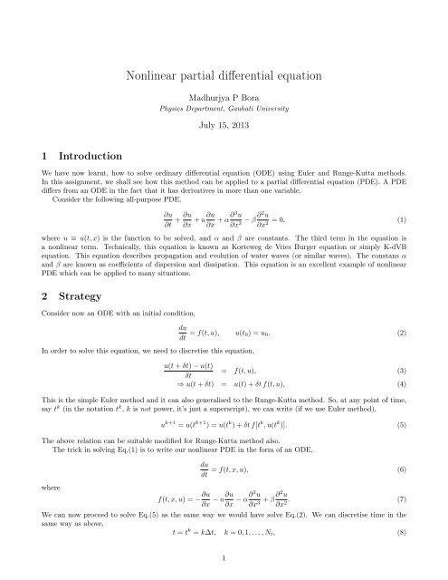
Figure 1: The sech solution of Eq.(12).where ∆t is the time step. The only difference is that we need to know the right hand side i.e. at every time step.How do we do that?To know the RHS of our equation, we first have to discretise the space. As our problem is 1-D in space, weconsider a one-dimensional grid in x, say from x = 0 to L with a grid space of ∆x. So, we divide our intervalx = [0, L] in N x divisions,x = x j = j∆x, j = 0, 1, . . . , N x − 1.At any point of space (x j ) and time (t k ), we can write,3 The boundaries and initial valuesu(x j , t k ) = u k j . (9)As you have realised that Eq.(1) is evolved in time from an initial time t = t 0 to a time in future (t = N t ). So, atone end, at t 0 , we know the values of all the variables and on the basis of that we are going to predict the values ata future time. In the same way we need to initialise our function u(t, x) in space at t = t 0 . In other words we needto allocate the values of all u 0 j at all the grid points x j. Once we allocate this values, the RHS of Eq.(7) at t = t 0becomes known and we can proceed to solve the equation in time to obtain the values u 1 j at each grid points. Inother words we have to advance N x numbers of ODEs at each time step. For example, if we are going to use Eulermethod, we can now write our problem as,u k+1j = u k j + ∆t f(t k , x j , u k j ), j = 0, 1, . . . , N x − 1. (10)The next question is that how are going to allocate the initial values u 0 j at each N x grid points? To know theinitial values, we need to find out values of u(t, x) which satisfies Eq.(1). For this purpose, we first set the coefficientβ = 0, which makes the equation look like,∂u∂t + ∂u∂x + u∂u ∂x + uα∂3 = 0. (11)∂x3 We now introduce a co-ordinate transformation z = x − V t, which transforms the equation to a moving frame withvelocity V ,−V dudz + dudz + udu dz + uαd3 = 0. (12)dz3 You can now check by direct substitution that,( √ )u(z) = 3(V − 1) sech 2 1 V − 12 z , (13)α2

satisfies Eq.(12). The above solution has the shape of a pulse (see Fig.1) in the moving frame. As we know thatour original equation has a nonzero dissipation term with nonzero coefficient β, we need to ensure that the abovesolution satisfies Eq.(1) when β ≠ 0. However, this term represents dissipation and physically it just damps theinitial pulse, so in principle, it should not affect the shape of the pulse. Also note that the pulse goes to zero at theboundaries i.e. at x = 0 and L, we need to ensure that at every time step, this condition is satisfied, otherwise wemight have unphysical effects. So, we introduce a periodic boundary condition that the boundary is periodic,at any point of time i.e. u k N x= u k 0.4 Computationsu(t, 0) = u(t, L), (14)Having determined the initial values u k 0 [from Eq.(13)], we now proceed to finalise the computational stages. As youwould realise that at every grid points, we need to know the values of u and its x-derivatives at every grid points.The values u k j are initialsed from Eq.(13) and then subsequently evolved in time using our favourite strategy (Euleror Runge-Kutta). To initialse the derivatives, we shall use the central difference scheme, as it is more accurate.4.1 The derivativesFirst we find the first derivatives at the interior points from j = 1, . . . , N x − 2,∂u(t k , x j )∂xThe second derivatives can be similarly found as,∂ 2 u(t k , x j )∂x 2≈ uk j+1 − uk j−1, j = 1, . . . , N x − 2. (15)2∆x≈ uk j+1 − 2uk j + uk j−1(∆x) 2 , j = 1, . . . , N x − 2. (16)The third derivatives can be found by applying the first derivative formula to the second derivative and need notwrite it separately. At the boundary points j = 0 and j = N x − 1, we invoke the periodic boundary condition (14).So, at j = 0, we have,and at j = N x − 1,4.2 Time steppingFor time stepping, we write now our original equation as,∂u(t k , x 0 )≈uk 1 − u k N x−1,∂x2∆x(17)∂ 2 u(t k , x 0 )∂x 2 ≈ uk 1 − 2u k 0 + u k N x−1(∆x) 2 (18)∂u(t k , x Nx−1)≈uk 0 − u k N x−2,∂x2∆x(19)∂ 2 u(t k , x Nx−1)∂x 2 ≈ uk 0 − 2u k N + x−1 uk N x−2(∆x) 2 . (20)dudt = − ddxFor Euler method, our time stepping becomes,)(u + u22 + uαd2 dx 2+ β d2 u= f(t, x, u). (21)dx2 u j ← u j + ∆t f(t, x j , u j ). (22)3

For 4th order Runge-Kutta, method, the stepping becomes,5 Putting it all together(1) k 1 ← f(u j , t) (23)(2) k 2 ← f(u j + 1 2 ∆t k 1, t + 1 )2 ∆t (24)(3) k 3 ← f(u j + 1 2 ∆t k 2, t + 1 )2 ∆t (25)(4) k 4 ← f (u j + ∆t k 3 , t + ∆t) (26)(5) u j ← u j + 1 6 ∆t (k 1 + 2k 2 + 2k 3 + k 4 ) (27)We are now ready to apply all the pieces together to solve Eq.(1). The algorithm is as follows:1. Initialse parameters(a) Define the length of simulation box L, say to 40.(b) Define total number of x intervals N x , say to 1000. So that ∆x = L/N x = 0.04.(c) Define time step ∆t, say to 0.001.(d) Initialise time t = 0.(e) Set the parameters α and β, say to 0.05.2. Initialise grid(a) Although we should use Eq.(13) to initialise the grid, we can use any Gaussian pulse say,u 0 j = 1 + exp[− 1 ]5 (x j − 20) 2The above initialisation produces a Gaussian pulse centered in the grid of length L = 40. You can adjustthis to suit your condition.(b) Initialse the derivatives according to relations (15)-(20).3. Begin time stepping(a) Apply the 4th order RK stepping, relations (23)-(27), to predict the new values of u j at the new timet = t + ∆t, i.e. u t j s.(b) Update the derivatives for u t j at the new time t = t + ∆t.(c) Update time t ← t + ∆t(d) Go back to step 3(a) unless you arrive at the final end time.4