An Ant-Based Algorithm for the Minimum Vertex Cover Problem

We approve the thesis of Muthubharathi Periannan.Date of SignatureThang N. BuiAssociate Professor of Computer ScienceChair, Mathematics and Computer Science ProgramsThesis AdvisorSukmoon ChangAssistant Professor of Computer ScienceLinda M. NullAssociate Professor of Computer Science

I grant The Pennsylvania State University the non-exclusive right to use this workfor the University’s own purposes and to make single copies of the work availableto the public on a not-for-profit basis if copies are not otherwise available.Muthubharathi Periannan

The Pennsylvania State UniversityThe Graduate SchoolAN ANT-BASED ALGORITHM FOR THEMINIMUM VERTEX COVER PROBLEMA Thesis inComputer SciencebyMuthubharathi Periannanc○ 2007 Muthubharathi PeriannanSubmitted in Partial Fulfillmentof the Requirementsfor the Degree ofMaster of ScienceDecember 2007

The thesis of Muthubharathi Periannan was reviewed and approved ∗ by the following:Thang N. BuiAssociate Professor of Computer ScienceChair, Mathematics and Computer Science ProgramsThesis AdvisorSukmoon ChangAssistant Professor of Computer ScienceLinda M. NullAssociate Professor of Computer Science∗ Signatures are on file in the Graduate School.

AbstractA vertex cover for a graph is a set of vertices, such that every edge in the graph isincident with at least one vertex in that set. The minimum vertex cover is definedas the vertex cover with the smallest size. The problem of finding the minimumvertex cover for a graph is well known to be NP-hard. This thesis provides anant-based algorithm for finding a small size vertex cover. The algorithm proceedsin two phases: exploration and construction. In the first phase, ants are usedto explore the graph and identify potential vertices that can be used in a vertexcover. In the construction phase, a greedy approach is used to build a vertexcover from the set of potential vertices. Local optimization techniques are used toimprove the quality of solutions and enhance the performance of the algorithm.Extensive experimental results show that the algorithm performs very well againstother approaches and produces close to optimal results.iii

Table of ContentsList of FiguresList of TablesAcknowledgementsviviiviiiChapter 1Introduction 1Chapter 2Preliminaries 32.1 Problem Definition . . . . . . . . . . . . . . . . . . . . . . . . . . . 32.2 Minimum Weight Vertex Cover Problem . . . . . . . . . . . . . . . 52.3 Ant Algorithms . . . . . . . . . . . . . . . . . . . . . . . . . . . . . 52.4 Previous Work . . . . . . . . . . . . . . . . . . . . . . . . . . . . . 7Chapter 3Ant-Based MVC Algorithm 103.1 Algorithm Overview . . . . . . . . . . . . . . . . . . . . . . . . . . 103.2 Initialization . . . . . . . . . . . . . . . . . . . . . . . . . . . . . . . 113.3 Exploration . . . . . . . . . . . . . . . . . . . . . . . . . . . . . . . 133.4 Pheromone Enhancement . . . . . . . . . . . . . . . . . . . . . . . . 153.5 Construction . . . . . . . . . . . . . . . . . . . . . . . . . . . . . . 163.6 Local Optimization . . . . . . . . . . . . . . . . . . . . . . . . . . . 17iv

3.6.1 Rebuild Vertex Cover Technique . . . . . . . . . . . . . . . . 193.6.2 Redundant Vertex Removal Technique . . . . . . . . . . . . 21Chapter 4Experimental Results 234.1 The BHOSLIB Instances . . . . . . . . . . . . . . . . . . . . . . . . 234.2 The DIMACS Benchmark Instances . . . . . . . . . . . . . . . . . . 244.3 The Random Graph Instances . . . . . . . . . . . . . . . . . . . . . 26Chapter 5Conclusion 28Appendix APerformance Tables for the AB–MVC Algorithm 30References 36v

List of Figures2.1 A graph of Papadimitriou and Steiglitz with k = 3. . . . . . . . . . 42.2 A 2-Approximation Algorithm for the MVC Problem. . . . . . . . 53.1 An Overview of the AB–MVC Algorithm. . . . . . . . . . . . . . . 123.2 Cascading Effect of the Preprocessing Step Solves the Graph . . . 133.3 Movement of an Ant Based on the Value of Movement Factor. . . . 143.4 One Step in the Ant Movement Algorithm. . . . . . . . . . . . . . 163.5 Construction Stage. . . . . . . . . . . . . . . . . . . . . . . . . . . 183.6 Overview of Local Optimization Stage. . . . . . . . . . . . . . . . . 193.7 Rebuild Vertex Cover Technique. . . . . . . . . . . . . . . . . . . . 203.8 Redundant Vertex Removal Technique. . . . . . . . . . . . . . . . 224.1 Solution Quality Comparison. . . . . . . . . . . . . . . . . . . . . . 244.2 Running Time Comparison. . . . . . . . . . . . . . . . . . . . . . . 254.3 Solution Quality Comparison. . . . . . . . . . . . . . . . . . . . . . 26vi

List of TablesA.1 AB–MVC results on BHOSLIB Instances. . . . . . . . . . . . . . . 30A.2 AB–MVC results on BHOSLIB Instances. . . . . . . . . . . . . . . 31A.3 AB–MVC results on BHOSLIB Instances. . . . . . . . . . . . . . . 31A.4 AB–MVC results on DIMACS Benchmark Instances. . . . . . . . . 32A.5 AB–MVC results on DIMACS Benchmark Instances. . . . . . . . . 33A.6 AB–MVC results on DIMACS Benchmark Instances. . . . . . . . . 34A.7 AB–MVC results on DIMACS Benchmark Instances. . . . . . . . . 34A.8 AB–MVC results on Random Graph Instances. . . . . . . . . . . . 35A.9 AB–MVC results on Random Graph Instances. . . . . . . . . . . . 35vii

AcknowledgementsThe foremost gratefulness is owed to my advisor, Dr. Thang Bui, without whoseguidance and persistent help this thesis would not have been possible. I feel honoredhaving studied under him for two years and would like to thank him for takingme as his student. His lectures in algorithms and graph theory have been the solemotivating force for my research. I sincerely hope and wish that I get a chance towork under him in the future.I am deeply indebted to all the professors in the department of ComputerScience with whom I have taken classes in these two years: Dr. Linda Null, Dr.Qin Ding, and Dr. Jefferson Hartzler. I would also like to thank Dr. SukmoonChang under whom I worked as a grader. My thanks likewise go to Dr. JeremyBlum, Dr. Thang Bui, Dr. Sukmoon Chang, Dr. Xianghua Deng, and Dr. LindaNull, for not only reviewing this thesis, but also enduring its defense.My warmest gratitude goes to my parents and sisters who have showered mewith nothing but love for all these years and without whose support my graduatestudies would have been an unfulfilled dream. They are the reason for whatever Iam today. This thesis is dedicated to them.viii

Chapter 1IntroductionA vertex cover of an undirected graph G = (V, E) is defined as a subset C of Vsuch that every edge in E is incident with at least one of the vertices in C. Thevertex cover with minimum cardinality is called the minmum vertex cover of G.The minimum vertex cover problem (MVC) is the problem of finding the minimumvertex cover in a graph and is well known to be NP-hard. Its corresponding decisionproblem is NP-complete. In fact, the decision problem appeared as one of the 21NP-complete problems in Richard Karp’s breakthrough paper [15].The MVC problem has attracted researchers and practitioners because of its intractablenature and because many difficult real-world problems can be formulatedas instances of the minimum vertex cover including problems in the field of bioinformatics.It can be used in the construction of phylogenetic trees, in phenotypeidentification, and in analysis of microarray data, just to name a few [19].The vertex cover problem can be proved to be NP-complete by a reductionfrom 3-SAT or, as Karp did, by a reduction from the Clique problem. In fact, evenapproximating optimal solutions within a factor of 1.3606 is NP-hard [7]. Therefore,heuristics are needed to find good solutions in a reasonable amount of time.Various techniques such as Genetic Algorithms, Kernelization, and Simulated Annealinghave been applied to the MVC problem [27, 24, 10].Ant Colony Optimization (ACO), a class of ant algorithms, was first proposedby Dorigo and colleagues [8, 9] as a multi-agent approach for solving difficult

1 INTRODUCTION 2combinatorial optimization problems like the traveling salesman problem (TSP)and the quadratic assignment problem (QAP). The Ant-Based (AB) approachused in this thesis is another variety of ant algorithms and has been used in recentyears to solve many graph optimization problems such as the k-cardinality tree [4],the degree constrained minmum spanning tree [5], and the maximum clique [3], toname a few.The MVC problem is naturally suited for AB approach, wherein the ants areused to explore the graph, identifying potential vertices based upon local information.Later, the information gathered by the ants is used to construct the vertexcover. Finally, local optimization techniques are employed to improve the qualityof the solutions and enhance the performance. Extensive experimental resultsshow that our approach is very competitive with other algorithms in both runningtime and solution quality.The rest of this thesis is organized as follows. Chapter 2 provides a formaldefinition of the problem, its generalization and description of previous works. Ourant-based algorithm is described in Chapter 3. Chapter 4 presents and comparesthe performance of this algorithm against existing algorithms on a set of benchmarkand random instances. Chapter 5 presents the conclusion of the thesis and suggestsideas for future research.

Chapter 2Preliminaries2.1 Problem DefinitionLet G = (V, E) be an undirected graph with vertex set V and edge set E. A vertexcover of G is then defined as a subset C of V that contains at least one of the twoend-points of every edge in E. The vertex cover with minimum cardinality is calledthe minimum vertex cover of G. Formally, the minimum vertex cover problem canbe stated as follows.Input: An undirected graph G = (V, E), where V is the vertex set and E is theedge set.Output: Smallest C ⊆ V such that ∀(u, v) ∈ E, u ∈ C or v ∈ C.Since we are interested in covering all edges of the graph by using as fewvertices as possible, one might be tempted to use a greedy approach. One suchgreedy algorithm operates by selecting a vertex u with the highest degree, i.e., avertex that is incident with the most number of edges, and adding it to the coverC. The edges that are covered by u are then removed from E. The procedure isrepeated until E is empty.However, this is not a good strategy as can be seen by considering Papadimitriouand Steiglitzs graphs [20], where the graph consists of three levels. The firsttwo levels always have the same number of vertices while the third level has twofewer vertices.

2 PRELIMINARIES 4Each vertex in the first level is connected to exactly one vertex in the secondlevel. While, there exists a complete bipartite graph between the vertices in leveltwo and three, i.e., every vertex in level two is connected to every vertex in levelthree. In general, such a graph consists of n vertices where n = 3k + 4 (k ≥ 1).Figure 2.1 shows a graph with k = 3. It is evident that the greedy algorithmdoes not return the optimal solution. In fact it can be shown that the algorithmperforms with a relative error that grows as fast as O(ln n) [20].a b c d e • • • • • level 1 (k + 2 vertices)f • g• h• i• j • level 2 (k + 2 vertices)k • • l m • level 3 (k vertices)Figure 2.1. A graph of Papadimitriou and Steiglitz with k = 3.However, another well-known greedy algorithm described in Figure 2.2, guaranteesto return a vertex cover with size no more than twice the size of the optimalsolution. This 2-approximation algorithm starts by randomly selecting an edge(u, v) from E. It then adds both end-points, u and v to the cover C. Finally, alledges incident with either u or v are removed from E. The entire procedure isrepeated until E is empty.It can be clearly seen that C is a vertex cover, as all the edges in E are covered.Let M be the set of edges selected by the algorithm. Then, M is a matching ofG, i.e., no two edges in M touch each other. Because the edges of M are disjoint,the minimum vertex cover must have at least one vertex from each edge in thismatching. Therefore, the size of the minimum vertex cover is at least the size ofM. But, the size of C is twice the size of M, as both end-points of every edge inM are added. This proves that the solution returned by the algorithm is no morethan twice the size of the optimal solution.

2 PRELIMINARIES 5Input: Graph G = (V, E)Output: A vertex cover C for G with size no morethan twice the size of the optimal vertex coverbeginC ← ∅while E is not emptyRandomly select an edge (u, v)Add u and v to CRemove all edges incident with either u or v from Eend-whilereturn CendFigure 2.2. A 2-Approximation Algorithm for the MVC Problem.2.2 Minimum Weight Vertex Cover ProblemGiven an undirected graph G = (V, E) with weights defined on the vertices, theminimum weight vertex cover problem (MWVC) is to find a vertex cover C of Gsuch that the sum of the weights of all nodes in C is minimum. Formally, theproblem can be stated as follows.Input: An undirected graph G = (V, E) where V is the vertex set and E is theedge set. A weight function w : V → Z + .Output: A subset C ⊆ V such that ∀(u, v) ∈ E, u ∈ C or v ∈ C and ∑ x∈C w(x)is minimum.The minimum vertex cover problem is a special instance of the minimum weightvertex cover problem. MVC is just an instance of MWVC where all the vertexweights are the same.2.3 Ant AlgorithmsBefore we describe our ant-based algorithm for the MVC problem, it might beuseful to review ant algorithms in general. Ant algorithms are a class of swarmintelligence systems, typically made up of a population of simple agents, called ants,

2 PRELIMINARIES 6interacting locally with one another and with their environment. Ant algorithmswere inspired by the observation of real ant colonies. Ants are social insects, thatis, insects that live in colonies and whose behavior is directed more to the survivalof the colony as a whole than to that of a single individual component of the colony.An important feature of ant colonies is their nature to find shortest pathsbetween their nest and the food source. While travelling from their nest to thefood source and on the way back, ants deposit a substance called pheromone onthe ground. It is nothing but a volatile chemical substance which can be detectedby other ants. So, when the next ant sets about in search of food from its nest,it is more inclined to choose paths marked by strong pheromone concentrations.These ants in turn will increase the pheromone concentration on that path evenmore. This will soon lead to the typical line of ants all following the same path.However, it should be noted that the pheromone evaporates as time goes by and apath that has been deserted for a while tends to vanish. This phenomenon helpsthe ants to explore and identify paths leading to different food sources.Ant algorithms can be broadly classified into two types: Ant colony optimization(ACO) and Ant-Based systems (AB). In ACO algorithms, a colony of artificialants collectively searches for good solutions to the optimization problem under consideration.Each ant builds a complete solution on its own. While building thesolution it collects information, both on the problem characteristics and on itsown performance. It then uses this information to modify the representation ofthe problem, as seen by the other ants. Travelling Salesman problem (TSP) wasthe first problem to which the ACO technique was applied because of its obvioususe of the ants’ ability to find the shortest path [6]. Other problems that havebeen the focus of ACO work include the quadratic assignment, network routing,vehicle routing and frequency assignment problems [17].In an ant-based system, each ant does not construct a complete solution butrather confines itself to a part of the problem space. It coordinates with otherants to identify a promising configuration that is later used for constructing thesolution. The distinct advantage of AB systems over ACO is the fact that the antsneed not possess knowledge of the problem space from a global perspective. Thismakes them more amenable to an implementation in a distributed environment.AB systems have been used to solve problems such as the k-cardinality tree [4] and

2 PRELIMINARIES 7the degree constrained minmum spanning tree [5] and have produced better resultswhen compared to other heuristics. Our algorithm is an ant-based approach andis described in detail in Chapter 3.2.4 Previous WorkThe minimum vertex cover problem has been studied for a long time because of itsimportance and its various applications in real life problems. The MVC has beentackled by both heuristics, which try to find solutions as close as possible to theoptimum solution, and by approximation algorithms that guarantee to producesolutions within specified bounds.We have previously mentioned that MVC is known to be NP-hard, and moreoverit cannot be approximated within a factor of 1.3606 unless P=NP [7]. A2-approximation algorithm has been discussed in the previous section. Improvingthis simple 2-approximation algorithm has been a non-trivial task. A numberof traditional approaches to MVC, typically with performance bounds close to 2,have been reported and are discussed in [11] and [18]. The best approximationalgorithm known, until recently, was published 20 years ago by Bar-Yehuda andEven [1]. They achieved an approximation factor of 2 − Θ(log log n/ log n). Thisfactor was reduced even further by Karakostas to 2 − Θ(1/ √ log n) [14].Various heuristic techniques such as genetic algorithms, simulated annealing,ant colony optimization and kernelization, have been applied to solve the MVCproblem in the recent past. In the mid 1990’s Khuri and Back implemented astraightforward genetic algorithm for the MVC problem [16]. They used a geneticalgorithm with proportional selection and two-point crossover and tested theirresults against the 2-approximation algorithm on randomly generated graphs. Thisis one of the very first heuristic technique to be developed and the aim of the paperwas to demonstrate that genetic algorithms can be used in a straightforward wayto find good approximate solutions for the minimum vertex cover problem.Simulated annealing has been used as a heuristic to solve the MVC problem byXu and Ma [27]. Annealing is a generic term denoting a treatment, consisting ofheating a component to a specific temperature, holding it at that temperature fora specified period of time, followed by cooling at a suitable rate. An optimization

2 PRELIMINARIES 8method that simulates the physical process of annealing by allowing the occasionalacceptance of less attractive solutions or values is called simulated annealing. Indetail, simulated annealing starts initially with an arbitrary solution and thenrepeatedly tries to make improvements to it locally. A better solution is alwaysaccepted, however a worse solution is accepted with a probability that decreasesexponentially with the ratio of decrease in the solution quality and the temperatureT. Xu and Ma had defined a new acceptance function for every vertex and hadtested their algorithm against a limited number of ten benchmark graphs and foundit to be achieving close to optimal solutions with a high probability [27].Richter, Helmert, and Gretton have developed a stochastic local search algorithm(SLS) for the MVC problem named COVER [21]. SLS Methods are popularmeans of solving hard combinatorial problems [12]. An SLS algorithm operatesby searching in a space of candidate solutions for a problem, where a candidatesolution may not satisfy all of the constraints required by a solution. The COVERalgorithm takes as input, a graph G = (V, E) and a parameter k, and searches fora vertex cover of size k for G. Its candidate solutions are subsets of the vertex setV with size k. The algorithm starts with an initial candidate solution and tries tobuild a valid vertex cover by exchanging vertices. The algorithm terminates whena valid solution is generated or the number of cycles has reached the maximumlimit. Richter, Helmert and Gretton have evaluated their performance against awide variety of benchmark graphs and have vastly improved on existing results.However, the performance of the algorithm is highly influenced by the additionalparameter k. In the absence of this parameter, there is a significant decline in thequality of solutions and a significant increase in running time.Shyu, Lin and Yin implemented an ant colony optimization algorithm, (ACO)for the minimum weight vertex cover problem (MWVC) [23]. Their algorithm aimsto identify a path that constitutes a vertex cover. To apply the ACO approachto meet the problem characteristics, they had transformed the original instanceof the graph into a complete graph, suitable for ants to traverse and composeapproximate solutions to MWVC. The theme of the paper was to introduce anddemonstrate the capability of ACO in dealing with MWVC. Their algorithm producedgood results for graphs with less than 50 vertices. However, as the size ofthe graph increased, the quality of the solutions decreased significantly. Gilmour

2 PRELIMINARIES 9and Dras have developed an algorithm named ACS, where a framework integratesstructural knowledge of the graph into the ACO metaheuristic [10]. The structureis determined through the notion of kernelization from the field of parameterizedcomplexity. They have tested their ACS algorithm against the same set of instancesthat was used by the ACO algorithm and have generated better resultswhen compared to the ACO algorithm.Recently, a hybrid heuristic for the MWVC problem was developed by Singhand Gupta [24]. Initially, a steady-state genetic algorithm is used to generate validvertex cover solutions. Later, a heuristic is applied to these solutions that tries toeliminate the redundant vertices from them. They have compared their algorithmagainst the ACO technique of Shyu, Lin and Yin and have produced better results.

Chapter 3Ant-Based MVC Algorithm3.1 Algorithm OverviewThis chapter describes our ant-based algorithm, called AB–MVC, for the MVCproblem. The principal idea of AB–MVC is to have a group of ants explore theproblem space and learn about the nature of the vertices. Later a vertex cover isbuilt using the knowledge gathered by the ants. The quality of this vertex coveris further improved by using local optimization techniques and finally, the bestsolution is returned.Ants are distributed at random, across various edges in the graph. Theseants then travel from one edge to another passing through vertices for a certainnumber of steps. As the ants cross a vertex, the pheromone content of that vertexgets increased and this increases the probability of the other ants to pass throughthe same vertex. The strategy used by the ants to select the edges to move tois designed in such a way that, vertices with high degree with respect to theirneighborhood are visited more frequently. These vertices, as they cover morenumber of edges in the graph, are considered to be potentially good vertices forthe vertex cover. Thus, potentially good vertices are likely to be crossed morefrequently and hence have a high pheromone content on them. These vertices arethen identified and are used to construct a vertex cover. The entire process isrepeated in cycles and a solution is computed in every cycle. After the stoppingcondition is met, the best solution computed is returned as a vertex cover for thegraph.

3 Ant-Based MVC Algorithm 11The algorithm consists of four main stages: initialization, exploration, construction,and optimization. In the initialization stage, the algorithm reads theinput file, stores the information in appropriate data structures and applies a preprocessingtechnique. Next, in the exploration stage, ants are allowed to explorethe graph and gather information about the problem space. In the constructionstage, using the knowledge gathered by the ants, we use a greedy approach toconstruct a vertex cover. Finally, this solution is passed on to the local optimizationstage, where we have two techniques to enhance the solution further. Thissolution is then compared to the best solution computed in previous cycles and isretained if better, else it is discarded. The algorithm terminates after a certainnumber of cycles or if the stopping criteria are met. Figure 3.1 broadly describesthe AB–MVC algorithm.3.2 InitializationAs the first step of initialization, the input graph is read and the informationis stored. Before we run the ant algorithm on this graph, a simple but efficientpreprocessing step is applied. In this step, we identify all the degree one verticesand add their neighbor to the cover C. Both the degree one vertex and its neighborare then removed from V. Also, all the edges that are incident with both thesevertices are removed from E. The entire procedure is repeated until there are nomore degree one vertex in the graph. It should be noted that the preprocessingstep can have a cascading effect on the input graph. In fact, this will solve theproblem optimally if the input graph is a tree.The idea behind this preprocessing step is that, for these edges to be coveredby the solution, one of their two end-points has to be a part of the vertex cover.Hence, it is ideal to have the end with degree greater than one in the solution, asit is more likely to cover other edges as well. Figure 3.2 illustrates this step. Byadding d to the vertex cover, we have covered the edges (d, b), (d, c), (d, e), and(d, f).Once preprocessing is complete, the ant algorithm is applied to the modifiedgraph, G = (V, E) returned by the preprocessing step. To start with, the verticesare assigned a uniform initial pheromone value. Then, based upon our initial

3 Ant-Based MVC Algorithm 12Input: Graph G = (V, E)Output: A vertex cover C of Gbegin// initialization stageC ← ∅bestC ← Vwhile a degree 1 vertex u exists // preprocessing stepv ← neighbor(u)C ← C ∪ {v}V ← V − {u, v}remove all edges incident with v from Eend-whilecopyE ← Eposition ants on randomly selected edgesinitialize the pheromone level of all verticeswhile stopping criteria not met// exploration stageE ← copyEfor step = 1 to numOfStepsfor each ant a // more details in Figure 3.4select an edge (u, v) for the ant a to move to and move it thereupdate the pheromone level for all verticesend-for// construction stage – more details in Figure 3.5compute coverFactor for all verticeswhile E is not emptyadd the vertex u with highest coverFactor to Cremove all edges incident with u from Erecompute coverFactor for all verticesend-while// local optimization – more details in Figure 3.7 and Figure 3.8C ← RebuildCover(C)C ← RedundantVertexRemoval(C)if |C| < |bestC| thenbestC ← Cevaporate pheromone level globallyend-whilereturn bestCendFigure 3.1. An Overview of the AB–MVC Algorithm.

3 Ant-Based MVC Algorithm 13a ••c• e•b• dFigure 3.2. Cascading Effect of the Preprocessing Step Solves the Graph•ftesting, the number of ants to explore the graph is set to one tenth of the numberof edges in G. However, we have a maximum and minimum limit on the numberof ants to avoid crowding or sparseness. The number of steps each ant will take inone cycle is set to one fourth of the number of vertices in G, so that there will beenough exploration in each cycle. Next, the ants are distributed across randomlyselected edges, such that no edge contains more than one ant. However, it shouldbe noted that there can be edges with no ants on them. Also, every ant has atabu list attached to it, so that it can remember the last ten vertices that it hascrossed. This list is set to null at the start of the algorithm. This completes theinitialization stage and the ants are ready to explore the graph.3.3 ExplorationIn the exploration stage, the ants tend to learn about the problem space by movingaround the graph, passing from one edge to another. The objective of this stageis to explore the graph and identify potentially good vertices that can be used forconstructing a vertex cover in the next stage.Every edge in the graph has a value called the movement factor, defined withrespect to the position of an ant. Let (s, u) and (u, v) be two edges in the graph.Let the pheromone level of a vertex v be denoted by τ[v]. Let an ant be present inthe edge (s, u). Then, the movement factor of the edge (u, v) with respect to the

3 Ant-Based MVC Algorithm 14•s•xantu • v ••t•ys and u are first level neighborsx and v are second level neighborsFigure 3.3. Movement of an Ant Based on the Value of Movement Factor.ant present in the edge (s, u), denoted by movFac[s, u, v], is a linear combinationof the pheromone values of its two end-points u and v, and is defined as follows.movFac[s, u, v] = α ∗ τ[u] + β ∗ τ[v]where α and β are weights such that α < β.The movement factor guides an ant in selecting the next edge it wants to moveto. The greater the movement factor of an edge is, the higher the chance thatedge gets selected. If an ant is currently present on the edge (s, u), then thepheromone value of v contributes more to the movement factor of the edge (u, v)when compared to u. On the other hand, if the ant is present on the edge (v, t),then the pheromone value of u has a greater influence on the value of the movementfactor of (u, v). Hence, an edge can have one of the two possible movement factorvalues, based upon the position of an ant.The reason for having the concept of a linear combination is intuitive and canbe explained with the help of Figure 3.3. In the current scenario, since the ant ispresent on the edge (s, u), u becomes its first level neighbor, whereas v is its secondlevel neighbor, meaning that the ant has to pass through u to get to v. It can beeasily noticed that at any point of time, an ant will always have only two first levelneighbors, the two end-points of the edge on which it is present. However, it canhave any number of second level neighbors, based on the degrees of its first levelneighbors. Hence, by forcing the second level neighbors to contribute more to themovement factor, we are making the ants select edges by looking one step ahead.This forward looking strategy helps the ants to better explore the graph.Each ant has a tabu list attached to it, so that it can remember the last ten

3 Ant-Based MVC Algorithm 15vertices that it has crossed. The tabu list is a circular queue data structure. Everytime when an ant tries to make a move, it checks its tabu list to make sure thatit has not crossed that same vertex in the past ten moves. If the vertex is notpresent in the list, it makes the move and then adds the vertex to the end of thelist. On the other hand, if it finds the vertex in its list, the ant tries to select adifferent path. It repeats this procedure until it makes a successful move or untilthe maximum number of steps has been reached. Figure 3.4 explains the stepsinvolved in the exploration stage.3.4 Pheromone EnhancementAfter all the ants complete one step, the pheromone level of the vertices thatthe ants have crossed is updated. We enhance the pheromone level of a vertexv, τ[v] based on two factors. The vertexVisitCt[v] is the total number of timesvertex v has been crossed by all ants in that step. This value is updated in eachstep. The second factor, degIdx[v] is defined as, the ratio of degree of vertex v tothe highest degree of its neighbor. This value remains a constant throughout theentire algorithm and is hence computed just once. Also, we have a threshold onthe pheromone level of all vertices, called maxPherm. If the pheromone level of avertex goes beyond the maxPherm value, it is reset to maxPherm. By doing this,we ensure that the difference in pheromone levels between vertices does not growunbound. The pheromone level of vertex v, denoted by τ[v], is updated as follows.τ[v] ← min{maxPherm, τ[v] + (degIdx[v] ∗ vertexVisitCt[v] ∗ initPherm)}The reason for including the vertexVisitCt in the pheromone enhancement isstraightforward. The more a vertex gets visited, the higher its pheromone levelbecomes. However, the idea behind having the degIndx is to ensure that a vertexv is assessed not only based on its degree but also based upon its neighborhood.This helps us to qualify a vertex with respect to its neighborhood.

3 Ant-Based MVC Algorithm 16beginfor each ant afor count = 1 to noOfAttemptsselect an edge (u, v) for ant a to move to, based on movement factor// assume that a reaches (u, v) by crossing vertex uif u /∈ a[tabulist] thenadd u to a[tabulist]move a to (u, v)vertexVisitCt[u] ← vertexVisitCt[u] + 1breakelseremove the first element from a[tabulist]end-ifend-forend-for// update pheromone level of all verticesfor each vertex vif vertexVisitCt[v] ≠ 0 thenτ[v] ← τ[v]+(degIdx[v]∗ vertexVisitCt[v]∗ initPherm)if τ[v] ≥ maxPherm thenτ[v] ← maxPhermend-forendFigure 3.4. One Step in the Ant Movement Algorithm.3.5 ConstructionIn the construction stage, the knowledge gathered by the ants is used to identify aset of candidate vertices and construct a vertex cover using them. The constructionalgorithm uses a greedy approach to select a vertex v and adds it to the cover.The edges that are covered by v are then removed from E. The entire procedureis repeated until E is empty.The candidate vertices are selected based upon a value called coverFactor. Thisvalue is a combination of two factors. The first factor is the pheromone content ofa vertex that is computed at the end of the exploration stage. The second factoris currDeg, which refers to the current degree of a vertex. The currDeg of a vertexv is defined as the number of edges incident with v at that point of time. Initially,

3 Ant-Based MVC Algorithm 17the value of currDeg is same as the degree of a vertex. The coverFactor of a vertexv is defined as follows.coverFactor[v] = α ∗ τ[v] + β ∗ currDeg[v],where α and β are weights.Initially, we build a candSet where all the vertices in V are sorted in a nonincreasingorder, based upon their coverFactor value. The first vertex v is thenselected and added to the cover C. We then remove v from the candSet. The edgesthat are incident with v are then removed from E. Since we have removed edgesfrom E, the currDeg value of all vertices is recalculated. Typically, the currDegof all the neighbors of v is reduced by 1. Next, the coverFactor of all the verticeswhose currDeg value has changed is recalculated. Finally, we rebuild the candSetbased on the current coverFactor value of all vertices. The algorithm proceedsby repeating the steps until a complete cover is formed. Figure 3.5 provides anoverview of the steps involved in the construction stage.The notion behind having a cover factor is to accomodate both the knowledgegathered by the ants as well as the current configuration of the graph. Also, thereason for dynamically updating the degree of a vertex is to ensure that the nextvertex to be added to the cover is a good vertex with respect to the current partialvertex cover generated. The vertex cover constructed is then passed onto the localoptimization stage for further improvement.3.6 Local OptimizationThe primary reason for having a local optimization stage is to improve the qualityof the solution and to enhance the performance of the algorithm by helping theants to converge on good solutions at a faster rate. In our AB–MVC algorithm,we have two local optimization techniques implemented. The first technique iscalled rebuild vertex cover technique, where we break the solution generated by theconstruction stage partially and try to rebuild a new vertex cover. In the redundantvertex removal technique, as the name implies, we try to get rid of redundantvertices from the solution generated by the rebuild vertex cover technique. The

3 Ant-Based MVC Algorithm 18begin// construction stageC ← ∅for each vertex vcoverFactor[v] ← α ∗ τ[v] + β ∗ currDeg[v]end-forcandSet ← vertex set V sorted in non-increasing order of coverFactorwhile E is not emptyadd the vertex v with highest coverFactor in candSet to Cremove the vertex v from candSetremove all edges incident with v from Efor each vertex u where u is a neighbor of vcurrDeg[u] ← currDeg[u] − 1coverFactor[u] ← τ[u]∗ currDeg[u]end-forcandSet ← candSet sorted in non-increasing order of coverFactorend-whilereturn CendFigure 3.5. Construction Stage.two techniques are explained in detail in the following sections.The entire local optimization stage runs in cycles, where the two techniquesare applied sequentially. Initially, C is copied into bestLocalC. At the beginning ofeach cycle, the rebuild vertex cover technique operates on the cover C, returned bythe construction algorithm. The new solution, localC, generated by this techniqueis then passed to the redundant vertex removal technique, where the redundantvertices are removed. If the size of this new localC is smaller than bestLocalC, thenwe copy localC into bestLocalC; otherwise it is discarded. The entire procedure isthen repeated in the next cycle. Finally, after all the cycles have been completed,the bestLocalC is returned. Figure 3.6 provides an overview of the steps involvedin the local optimization stage.

3 Ant-Based MVC Algorithm 193.6.1 Rebuild Vertex Cover TechniqueThis is the first local optimization technique that we use to improve the qualityof the solutions. In this method, we break the vertex cover C partially and try torebuild a new cover. This new cover is then passed to the next technique, whereredundant vertices get removed.Recall that in the construction stage, every time a vertex gets added to thecover, the edges incident with it are removed from the graph and the currDeg ofall the other vertices is recalculated. Consider the scenario where a vertex v has adegree x. Before the construction algorithm begins, the currDeg value of v is equalto x. However, as the algorithm proceeds, the currDeg value of v might decreaseif the neighbors of v get added to the cover. This results in v having a smallercoverFactor value and hence gets pushed to the bottom of the candSet. Becauseof this phenomenon, the order in which vertices are added to the cover becomesa key factor. Therefore, by breaking the cover partially, this technique presentsa new partial vertex cover and a candSet of vertices from which a possible newvertex cover can be built.Input: Vertex cover C of GOutput: A new vertex cover bestLocalC such that |bestLocalC| ≤ |C|beginbestLocalC ← CcycleCount ← 0while cycleCount ≤ noOfCycleslocalC ← RebuildCover(C)localC ← RedundantVertexRemoval(C)if |localC| ≤ |bestLocalC| thenbestLocalC ← localCend-ifcycleCount ← cycleCount+1end-whilereturn bestLocalCendFigure 3.6. Overview of Local Optimization Stage.

3 Ant-Based MVC Algorithm 20begin// rebuild vertex cover techniqueA ← ∅removeCt ← 0.25 ∗ |C|while removeCt > 0select a vertex v from C at random and proportional to its currDeg valueif v /∈ A thenA ← A ∪ {v}removeCt ← removeCt − 1end-ifend-whilelocalC ← C − Afor each vertex v in localCremove all the edges incident with v from Eend-forfor each vertex v in V − localCrecalculate currDeg[v]recalculate coverFactor[v]end-forBuild a candidate set of vertices candSet based on coverFactor valuewhile E is not emptyadd the vertex v with highest coverFactor in candSet to localCremove the vertex v from candSetremove all edges incident with v from Efor each vertex u where u is a neighbor of vcurrDeg[u] ← currDeg[u] − 1coverFactor[u] = α ∗ τ[u] + β ∗ currDeg[u]end-forrebuild candSet based on coverFactor valueend-whilereturn localCendFigure 3.7. Rebuild Vertex Cover Technique.The rebuild vertex cover technique operates on the vertex cover C, returned bythe construction algorithm. The first step would be to remove a set of A vertices,A ⊂ C, from C and copy the remaining vertices into localC, which becomes our newpartial vertex cover. The size of A is set to 20%−25% of the size of C. The verticesto be removed are selected in such a way that vertices with a higher currDeg value

3 Ant-Based MVC Algorithm 21are more likely to be selected, compared to vertices with lower currDeg value.Next, we recalculate the currDeg and coverFactor for all the non-cover vertices,i.e., vertices in (V − localC). It should be recalled that the coverFactor value ofa vertex is a linear combination of two factors. The first factor is the pheromonecontent of a vertex and the second factor is the currDeg of a vertex. We modifythe weights on these two factors so that the currDeg value has a higher influencewhen compared to the pheromone content.Finally, we rebuild a complete cover, using the current partial vertex cover,localC, and a new candSet of vertices. The new, complete cover localC is thenpassed to the next technique, where the redundant vertices are removed from it.Figure 3.7 explains the steps involved in the rebuild vertex cover technique.3.6.2 Redundant Vertex Removal TechniqueIn this technique, we examine the solution returned by the rebuild technique andtry to identify the set of vertices that are redundant and hence, removing themfrom the cover. The idea is based on a similar technique used by Singh and Guptain their hybrid heurisitc algorithm for the MWVC problem [24], where they selecta set of vertices from the vertex cover, all of whose edges are covered by othervertices in the cover. They then randomly select a vertex from this set, having themaximum ratio of weight to degree, and remove it from the cover.The set of redundant vertices can be easily identified by scanning through thecurrDeg value of all the vertices in the solution. It can be recalled that the currDegvalue of a vertex gets updated everytime a neighboring vertex gets added to thecover. Hence, it is evident that the currDeg of all the vertices not present in thesolution will always be zero, as all the edges that are incident with the non-coververtices are covered by vertices that are a part of the solution.However, it is also possible for some vertices in the cover to have a currDegvalue of zero. These are the potential candidates for redundant vertices. Initially,when a vertex v is added to the cover, it might be the only vertex covering theedges incident with it. However, as the construction algorithm proceeds, othervertices get added to the cover and these new vertices might also be covering theedges incident with v. If there exists a scenario where all the edges incident with v

3 Ant-Based MVC Algorithm 22begin// redundant vertex removal techniquelocalC new ← localCfor each vertex v in localC such that currDeg[v] = 0localC temp ← localClocalC temp ← localC − {v}for each vertex u in localC where u is a neighbor of vcurrDeg[u] ← currDeg[u] + 1end-forwhile there exists a vertex s in localC temp such that currDeg[s] = 0localC temp ← localC temp − {s}for each vertex t in localC temp where t is a neighbor of scurrDeg[t] ← currDeg[t] + 1end-forend-whileif |localC temp | < |localC new | thenlocalC new ← localC tempend-ifend-forreturn localC newendFigure 3.8. Redundant Vertex Removal Technique.are covered by other vertices in the solution, then the currDeg value of v becomeszero. Therefore, v becomes a redundant vertex and hence can be removed fromthe cover C.However, it should be noted that all vertices with currDeg value of zero cannotbe removed from the cover. Consider the case where vertices u and v are part of thecurrent solution and have their currDeg value as zero. If there exists an edge (u, v)in E, then the only two vertices covering this edge are u and v. Therefore, at leastone of the two vertices has to be retained in the cover to maintain the correctnessof the solution. Thus, the aim of the algorithm is to remove the maximum numberof vertices, from the set of potential candidates for redundant vertices withoutviolating the validity of the solution. Figure 3.8 explains the redundant vertexremoval technique.

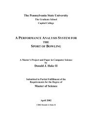
Chapter 4Experimental ResultsIn this chapter, we describe the results of running AB–MVC algorithm on an extensiveset of benchmark graphs and randomly generated graphs. In Section 4.1we report our results on the BHOSLIB benchmark suit [25], a set of graphs with“hidden optimal solutions” that are specifically designed to be hard to solve. InSection 4.2, we evaluate our performance on the complement graphs of the SecondDIMACS Implementation Challenge for the maximum clique problem [13]. Section4.3 reports our results on running AB–MVC on randomly generated graphs.Our AB–MVC algorithm was implemented in C++ and run on a 3.06GHz IntelXeon processor with 4GB of RAM running the Linux operating system. To obtainour results, the algorithm was run for 50 times on each instance.4.1 The BHOSLIB InstancesThe BHOSLIB problems (“Benchmarks with Hidden Optimal Solutions”) [25] resultfrom translating binary Boolean Satisfiability problems that were generatedrandomly according to the model RB [26]. The satisfiability versions of thesebenchmarks are guaranteed to be satisfiable, and the model parameters were setto such values that the instances are in the phase transition area of model RB, anew type of random CSP model. They have been proven to be hard both theoreticallyand in practice [26].The problem instances are grouped by size into 8 groups, with five graphs pergroup, where all graphs of a group have the same number of vertices and edges.

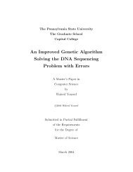
4 Experimental Results 24Figure 4.1. Solution Quality Comparison.The results of running AB–MVC on these graphs are shown in Tables A.1, A.2,and A.3. To compare our results, we tested it against the COVER algorithmof Richter, Helmert, and Gretton [21] and the ant colony optimization algorithm(ACS) of Gilmour and Dras [10].AB–MVC was able to identify solutions that were within the range of 1% tothe optimal solutions. The quality of the solutions generated were much betterwhen compared to the results of ACS. COVER was able to identify the optimalsolution in most cases, however the running time of COVER was much largerwhen compared to that of AB–MVC. The standard deviation from the optimalvertex cover for all the three algorithms, for the eight different groups of graphs ispresented in Figure 4.1. Figure 4.2, that compares the running time of AB–MVCwith COVER proves that we had a fair balance between the quality of solutionsand running time, unlike the VCOVER algorithm.4.2 The DIMACS Benchmark InstancesThe DIMACS benchmark instances are taken from the Second DIMACS ImplementationChallenge (1992–1993) [13], a competition targeting the maximum clique,

4 Experimental Results 25Figure 4.2. Running Time Comparison.graph colouring, and satisfiability problems. The problem of finding the maximumclique in a graph is closely related to the minimum vertex cover problem. A cliquein a graph G is defined as a subset A ⊆ V where every two vertices in A are joinedby and edge in E. The maximum clique problem is to find a clique of maximumsize in G. The complement or inverse of a graph G is defined as a graph G ∗ , on thesame vertices of G, such that two vertices of G ∗ are adjacent if and only if they arenot adjacent in G. It is evident that if A is a clique in G then, V − A is a vertexcover in G ∗ .The benchmark set is comprised of 80 problems from a variety of classes. TheC-fat family is a set of graphs based on fault diagnosis problems. The Johnsonand Hamming classes of graphs are based on coding theory. Problems based onKeller’s conjecture on tilings using hypercubes are reflected in the Keller instances.In addition, there are graphs generated randomly according to various models.For example, the Brock family is generated by explicitly incorporating low-degreevertices into the cover, in order to defeat algorithms that search greedily withrespect to vertex degrees [2]. The sizes of the graphs range from less than 30vertices and approximately 200 edges to more than 3000 vertices and 5, 000, 000edges.

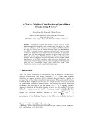
4 Experimental Results 26Figure 4.3. Solution Quality Comparison.The AB–MVC algorithm was run on the complement graph of these instances.To compare our results, we tested it against the COVER algorithm. AB–MVCwas able to successfully identify the optimal solutions in most classes of graphs.In the other cases where our algorithm failed to identify the optimal solutions,we obtained results with a standard deviation of less than 2%, with respect tothe optimal value. Figure 4.3 presents the standard deviation from the optimalvertex cover for the two algorithms. It was observed that for graphs with lowedge densities, AB–MVC was able to identify the optimal solution at least once.However, most of the time, the algorithm got stuck at a local optima and could notproceed any further. This is inferred from the relatively larger standard deviationvalues for classes of graphs like gen, san and sanr. The results of running AB–MVCand COVER on these graphs are shown in Tables A.4, A.5, A.6, and A.7,4.3 The Random Graph InstancesIn order to assess the effectiveness of the proposed algorithm, extensive simulationswere carried out on randomly generated graphs with known minimum vertexcover. The random graph instances are generated using the procedure describedby Sanchis [22]. The random graph generator accepts the number of vertices, n,

4 Experimental Results 27edge density, d, and size of the minimum vertex cover, c as input. It partitionsn into k parts, where k = n − c. Next, we make each of these k partitions into aclique and include all but one vertex from each of these cliques in our minimumvertex cover. Finally, additional edges are added to the graph in such a way thatat least one of their end-points belongs to the vertex cover. Using this method, wehave generated a graph of size n, with edge density d and minimum vertex coverof size c.The problem instances are grouped by size into 5 sets, with the number ofvertices ranging from 50 − 500. AB–MVC was run for 50 times on each of theseinstances and the results were tested against the COVER algorithm. Both AB–MVC and COVER were able to identify the optimal solution for all the test cases.However the running time of AB–MVC was much less when compared to thetime taken by COVER. The results of running AB–MVC on these random graphinstances are shown in Tables A.8 and A.9.

Chapter 5ConclusionIn this thesis, we have analyzed and studied the minimum vertex cover problemand the various heuristics that have been applied to solve it in the past. We havedesigned and implemented an ant-based algorithm for solving the MVC problem,and the experimental results show that the AB–MVC algorithm produces competitiveresults. Also, the running time of AB–MVC is less than 10% of the timetaken by COVER. Thus, AB–MVC has a fair balance between quality of solutionsand running time.A notable advantage of AB–MVC is the fact that it produces quality solutionson all classes of graphs without the need for tuning the parameters based onindividual instances. The AB–MVC algorithm is very flexible and has variousnovel techniques such as graph preprocessing, tabu lists, and greedy-based localoptimization techniques that contribute support to the ants.In general, it was observed that the quality of solutions of AB–MVC for graphswith low edge densities was relatively aberrant. This could be inferred by thestandard deviation values for graphs belonging to sanr and gen families. Thereason for this behavior is because the algorithm occasionally gets stuck at a localoptima and is not able to move further.Currently, the exploration stage operates by looking at two levels of the neighborhood.Future investigations could include looking beyond two levels of theneighborhood. Further parameter tuning such as modifying the number of stepsin a cycle, the number of ants, the size of the tabu list, and the value of the weightsused might also yield a combination of settings that produces better results. Also

5 Conclusion 29a parametric study would yield insight into the performance of the algorithm andhow it can be further improved.Because of the generic framework of AB–MVC, another area of follow up wouldbe to modify the AB–MVC algorithm to solve the minimum weight vertex coverproblem. The movement factor of an edge can be computed differently by includingthe weights of its two end-points. This will guide the ants to select vertices, basedon their weights. Finally, the local optimization techniques can be modified to suitthe problem.Given a graph G = (V, E), a dominating set D is a subset of V such that anyvertex not in D is adjacent to at least one vertex in D. The problem of finding thesmallest dominating set is called the minimum connected dominating set problem(MCDS). Our AB–MVC algorithm can be easily modified and applied to solve theMCDS problem by changing the construction algorithm to build a dominating setinstead of a vertex cover.Finally, because of the nature of ant-based systems, our algorithm is conduciveto parallel implementation. Using a parallel algorithm should greatly reduce therunning time, making it possible to easily find solutions for larger graph instances.

Appendix APerformance Tables for theAB–MVC AlgorithmTable A.1. AB–MVC results on BHOSLIB Instances.AB–MVC 50 runs ACS COVERInstance |V | |E| |C| ∗ best avg σ (sec) avg avg (sec)frb30-15-1 450 17827 420 423 423.8 0.69 122.9 424.0 420 1160.4frb30-15-2 450 17874 420 423 423.9 0.78 116.2 424.5 420 1174.5frb30-15-3 450 17809 420 423 423.5 0.50 113.3 424.6 420 1189.4frb30-15-4 450 17831 420 423 423.8 0.48 112.8 424.0 420 1173.7frb30-15-5 450 17794 420 423 423.7 0.46 111.6 423.6 420 1181.9frb35-17-1 595 27856 560 564 564.3 0.46 222.5 565.5 560 1640.6frb35-17-2 595 27847 560 564 564.6 0.47 215.4 566.5 560 1654.2frb35-17-3 595 27931 560 564 564.5 0.50 217.1 564.4 560 1680.1frb35-17-4 595 27842 560 564 564.6 0.49 215.3 565.5 560 1667.8frb35-17-5 595 28143 560 564 564.6 0.47 215.2 564.1 560 1681.4t avgt avgInstance: Name of the graph|V |: Number of vertices in the graph.|E|: Number of edges in the graph.|C| ∗ : Size of optimal Cover for the graph.best: Size of best cover generated.avg: Average size of the covers generated.σ: Standard deviation of the covers generated.t avg : Average time taken to compute the solution.

5 Conclusion 31Table A.2. AB–MVC results on BHOSLIB Instances.AB–MVC 50 runs ACS COVERInstance |V | |E| |C| ∗ best avg σ (sec) avg avg (sec)frb40-19-1 760 41314 720 725 725.6 0.47 349.4 725.6 721 2498.6frb40-19-2 760 41263 720 726 726.3 0.47 350.3 726.8 720 2476.3frb40-19-3 760 41095 720 726 726.3 0.49 349.6 727.6 720 2481.7frb40-19-4 760 41605 720 726 726.4 0.50 348.1 726.1 721 2498.5frb40-19-5 760 41619 720 725 725.6 0.49 348.9 725.3 721 2492.3frb45-21-1 945 59186 900 906 906.3 0.61 564.6 908.2 902 3721.6frb45-21-2 945 58624 900 906 906.4 0.62 573.2 908.5 902 3710.5frb45-21-3 945 58245 900 906 907.1 0.80 568.9 908.3 903 3712.3frb45-21-4 945 58549 900 906 906.9 0.73 581.2 908.4 901 3703.7frb45-21-5 945 58579 900 906 906.6 0.66 589.8 909.1 902 3704.5t avgt avgTable A.3. AB–MVC results on BHOSLIB Instances.AB–MVC 50 runs ACS COVERInstance |V | |E| |C| ∗ best avg σ (sec) avg avg (sec)frb50-23-1 1150 80072 1100 1109 1109.7 0.58 659.2 1110.4 1105 4815.3frb50-23-2 1150 80851 1100 1107 1108.4 0.68 663.6 1109.7 1107 4827.4frb50-23-3 1150 81068 1100 1107 1107.3 0.60 672.4 1108.3 1106 4809.8frb50-23-4 1150 80258 1100 1109 1109.1 0.43 667.0 1109.6 1104 4807.5frb50-23-5 1150 80035 1100 1107 1107.8 0.84 667.5 1110.3 1106 4821.6frb53-24-1 1272 94227 1219 1228 1228.2 0.43 1084.4 1229.9 1223 7040.6frb53-24-2 1272 94289 1219 1227 1227.4 0.49 1102.7 1229.3 1225 7069.8frb53-24-3 1272 94127 1219 1228 1228.1 0.62 1097.7 1031.6 1226 7024.7frb53-24-4 1272 94308 1219 1227 1227.5 0.50 1109.3 1030.5 1225 7019.3frb53-24-5 1272 94226 1219 1228 1228.2 0.66 1104.5 1031.8 1226 7125.7frb56-25-1 1400 109676 1344 1354 1354.7 0.56 1219.3 1356.8 1348 15789.4frb56-25-2 1400 109401 1344 1354 1355.0 0.69 1238.2 1355.7 1349 15694.2frb56-25-3 1400 109379 1344 1354 1354.1 0.47 1215.7 1355.6 1347 15756.9frb56-25-4 1400 110038 1344 1353 1353.7 0.81 1222.6 1354.8 1347 15801.3frb56-25-5 1400 109601 1344 1353 1353.3 0.57 1232.1 1354.6 1348 15655.7frb59-26-1 1534 126555 1475 1484 1484.2 0.65 1854.2 1486.8 1477 18611.3frb59-26-2 1534 126163 1475 1484 1484.7 0.82 1879.6 1486.4 1478 18589.5frb59-26-3 1534 126082 1475 1484 1484.3 0.66 1833.7 1487.8 1480 18605.1frb59-26-4 1534 127011 1475 1485 1485.1 0.71 1865.5 1487.3 1479 18704.8frb59-26-5 1534 125982 1475 1485 1485.7 0.59 1895.9 1487.3 1478 18523.5t avgt avg

5 Conclusion 32Table A.4. AB–MVC results on DIMACS Benchmark Instances.AB–MVC 50 runst avgCOVERInstance |V | |E| |C| ∗ best avg σ (sec) avg (sec)brock200 1 200 5066 179 180 180.2 0.23 24.1 179 768.2brock200 2 200 10024 188 190 190.1 0.31 29.8 189 795.7brock200 3 200 7852 185 186 186.7 0.35 27.6 185 774.6brock200 4 200 6811 183 184 184.2 0.27 25.2 183 798.2brock400 1 400 20077 373 376 376.3 0.54 118.4 374 2145.9brock400 2 400 20014 371 374 374.9 0.45 117.9 372 2198.1brock400 3 400 20119 369 372 372.1 0.29 123.5 369 2184.8brock400 4 400 20035 367 369 369.5 0.38 119.8 367 2177.7brock800 1 800 112095 777 781 781.4 0.56 513.7 779 4678.6brock800 2 800 111434 776 779 779.7 0.66 516.8 778 4624.4brock800 3 800 112267 775 778 778.2 0.32 509.3 776 4633.9brock800 4 800 111957 774 778 778.8 0.81 520.6 775 4651.2C125.9 125 787 91 91 91 0.0 2.0 91 656.3C250.9 250 3141 206 206 206 0.0 14.2 206 902.4C500.9 500 12418 443 447 447.3 0.65 157.3 443 1478.9C1000.9 1000 49421 932 940 940.8 0.71 305.8 932 15892.6C2000.5 2000 999164 1984 1988 1988.7 0.61 1856.4 1984 27546.2C2000.9 2000 199468 1922 1930 1930.5 0.72 1513.5 1922 21489.7t avg

5 Conclusion 33Table A.5. AB–MVC results on DIMACS Benchmark Instances.AB–MVC 50 runst avgCOVERInstance |V | |E| |C| ∗ best avg σ (sec) avg (sec)c-fat200-1 200 18366 188 188 188 0.0 79.8 188 1612.2c-fat200-2 200 16665 176 176 176 0.0 75.4 176 1598.7c-fat200-5 200 11427 142 142 142 0.0 63.2 142 1549.1c-fat500-1 500 120291 486 486 486 0.0 589.6 486 4489.7c-fat500-2 500 115611 474 474 474 0.0 567.2 474 4387.3c-fat500-5 500 101559 436 436 436 0.0 555.3 436 4391.6c-fat500-10 500 78123 374 374 374 0.0 537.9 374 4401.2gen200 p0.9 44 200 1990 156 156 158.5 3.53 24.5 156 1543.6gen200 p0.9 55 200 1990 145 145 147.1 2.91 26.9 145 1553.8gen400 p0.9 55 400 7980 345 345 348.7 3.62 132.3 345 2476.7gen400 p0.9 65 400 7980 335 335 339.2 3.47 149.8 335 2423.1gen400 p0.9 75 400 7980 325 325 328.9 3.12 140.3 325 2445.5hamming6-2 64 192 32 32 32 0.0 0.71 32 84.3hamming6-4 64 1312 60 60 60 0.0 5.93 60 143.7hamming8-2 256 1024 128 128 128 0.0 5.86 128 865.9hamming8-4 256 11776 240 240 240 0.0 85.3 240 1157.3hamming10-2 1024 5120 512 512 512 0.0 72.7 512 2412.2hamming10-4 1024 89600 984 988 988.4 0.547 949.8 986 3457.6johnson8-2-4 28 168 24 24 24 0.0 0.82 24 43.2johnson8-4-4 70 560 56 56 56 0.0 1.97 56 183.1johnson16-2-4 120 1680 112 112 112 0.0 9.86 112 297.9johnson32-2-4 496 14880 480 480 480 0.0 293.5 480 2351.9t avg

5 Conclusion 34Table A.6. AB–MVC results on DIMACS Benchmark Instances.AB–MVC 50 runst avgCOVERInstance |V | |E| |C| ∗ best avg σ (sec) avg (sec)keller4 171 5100 160 160 160 0.0 17.9 160 985.7keller5 776 74710 749 749 749 0.0 154.6 749 2364.9MANN a9 45 72 29 29 29 0.0 0.21 29 15.9MANN a27 378 702 252 252 252 0.0 68.6 252 756.3MANN a45 1035 1980 690 694 694.3 0.63 278.5 692 7568.9MANN a81 3321 6480 2221 2227 2227.2 0.31 608.3 2225 15672.1p hat300-1 300 33917 292 292 292 0.0 151.2 292 1099.3p hat300-2 300 22922 275 275 275 0.0 115.3 275 1052.2p hat300-3 300 11460 264 264 264 0.0 62.7 264 1014.6p hat500-1 500 93181 491 491 491 0.0 230.2 491 1810.2p hat500-2 500 61804 464 464 464 0.0 215.7 464 1798.9p hat500-3 500 30950 450 450 450 0.0 241.4 450 1754.1p hat700-1 700 183651 689 689 689 0.0 324.8 689 2098.7p hat700-2 700 122922 656 656 656 0.0 337.2 656 2020.5p hat700-3 700 61640 638 638 638 0.0 289.3 638 1984.6p hat1000-1 1000 377247 990 990 990 0.0 627.8 990 3642.4p hat1000-2 1000 254701 954 954 954 0.0 612.5 954 3601.1p hat1000-3 1000 127754 932 932 932 0.0 597.2 932 3547.8p hat1500-1 1500 839327 1488 1488 1488 0.0 827.7 1488 14932.6p hat1500-2 1500 555290 1435 1435 1435 0.0 814.9 1435 14869.4p hat1500-3 1500 277006 1406 1406 1406 0.0 795.2 1406 14257.2t avgTable A.7. AB–MVC results on DIMACS Benchmark Instances.AB–MVC 50 runst avgCOVERInstance |V | |E| |C| ∗ best avg σ (sec) avg (sec)san200 0.7 1 200 5970 170 172 173.3 2.87 25.1 170 713.7san200 0.7 2 200 5970 182 183 184.9 2.69 24.7 182 734.9san200 0.9 1 200 1990 130 130 130 0.0 26.3 130 692.5san200 0.9 2 200 1990 140 140 140 0.0 24.3 140 683.6san200 0.9 3 200 1990 156 156 156 0.0 25.6 156 676.4san400 0.5 1 400 39900 387 390 391.1 1.78 198.6 389 2381.1san400 0.7 1 400 23940 360 362 363.5 1.65 189.5 361 2396.3san400 0.7 2 400 23940 370 374 374.7 1.51 192.1 371 2405.6san400 0.7 3 400 23940 378 382 382.9 1.82 212.4 379 2390.7san400 0.9 1 400 7980 300 300 300 0.0 112.5 300 2288.5san1000 1000 249000 985 990 991 0.73 753.7 989 4972.8sanr200 0.7 200 6032 182 183 184.2 1.44 23.5 183 788.2sanr200 0.9 200 2037 158 158 159.3 1.3 18.5 159 612.1sanr400 0.5 400 39816 387 387 388.1 1.43 203.3 388 2134.9sanr400 0.7 400 23931 379 380 381.7 1.50 193.5 380 2112.5t avg

5 Conclusion 35Table A.8. AB–MVC results on Random Graph Instances.AB–MVC 50 runst avgCOVERInstance |V | |E| |C| ∗ best avg σ (sec) avg (sec)graph50-01 50 612 30 30 30 0.0 0.95 30 120.3graph50-02 50 490 30 30 30 0.0 0.89 30 123.1graph50-03 50 735 30 30 30 0.0 0.91 30 122.5graph50-04 50 612 40 40 40 0.0 0.90 40 121.7graph50-05 50 490 27 27 27 0.0 0.85 27 123.6graph50-06 50 857 38 38 38 0.0 0.87 38 122.2graph50-07 50 735 35 35 35 0.0 0.82 35 124.1graph50-08 50 612 29 29 29 0.0 0.93 29 120.9graph50-09 50 980 40 40 40 0.0 0.89 40 121.1graph50-10 50 612 35 35 35 0.0 0.87 35 124.5graph100-01 100 3465 60 60 60 0.0 20.8 60 198.7graph100-02 100 2475 65 65 65 0.0 19.5 65 201.4graph100-03 100 3465 75 75 75 0.0 23.4 75 204.6graph100-04 100 3960 60 60 60 0.0 21.4 60 199.7graph100-05 100 1980 60 60 60 0.0 18.4 60 201.2graph100-06 100 3960 80 80 80 0.0 22.8 80 205.8graph100-07 100 4207 65 65 65 0.0 28.7 65 203.9graph100-08 100 3712 75 75 75 0.0 25.6 75 202.2graph100-09 100 4207 85 85 85 0.0 24.2 85 204.6graph100-10 100 4207 70 70 70 0.0 25.6 70 205.3t avgTable A.9. AB–MVC results on Random Graph Instances.AB–MVC 50 runst avgCOVERInstance |V | |E| |C| ∗ best avg σ (sec) avg (sec)graph200-01 200 9950 150 150 150 0.0 65.4 150 812.5graph200-02 200 15920 125 125 125 0.0 67.3 125 895.7graph200-03 200 14925 175 175 175 0.0 68.6 175 889.6graph200-04 200 15920 140 140 140 0.0 65.9 140 875.2graph200-05 200 9950 150 150 150 0.0 62.7 150 854.1graph250-01 250 15562 150 150 150 0.0 72.1 150 1010.2graph250-02 250 23343 175 175 175 0.0 78.4 175 1057.8graph250-03 250 24900 200 200 200 0.0 81.7 200 1065.2graph250-04 250 24900 220 200 220 0.0 79.3 220 1058.7graph250-05 250 15562 200 200 200 0.0 69.2 200 998.5graph500-01 500 62375 350 350 350 0.0 510.6 350 2241.3graph500-02 500 99800 400 400 400 0.0 517.8 400 2237.4graph500-03 500 93562 375 375 375 0.0 521.2 375 2186.7graph500-04 500 99800 300 300 300 0.0 518.6 300 2285.1graph500-05 500 93562 290 290 290 0.0 515.7 290 2255.2t avg

References[1] Bar-Yehuda, R., and S. Even. “A Local-Ratio Theorem for Approximatingthe Weighted Vertex Cover Problem,” Annals of Discrete Mathematics, 25,1985, pp. 27–45.[2] Brockington, M. and J. C. Culberson, “Camouflaging Independent Sets inQuasi-Random Graphs,” Cliques, Coloring and Satisfiability: Second DI-MACS Implementation Challenge, 1996, pp. 75–88.[3] Bui, T. N. and J. R. Rizzo, Jr., “Finding Maximum Cliques with DistributedAnts,” Proceedings of the Genetic and Evolutionary Computation Conference(GECCO 2004), Lecture Notes in Computer Science, 3102, 2004, pp. 24–35.[4] Bui, T. N. and G. Sundarraj, “Ant System for the k-Cardinality Tree Problem,”Proceedings of the Genetic and Evolutionary Computation Conference(GECCO 2004), Lecture Notes in Computer Science, 3102, 2004, pp. 36–47.[5] Bui, T. N. and C. Zrncic, “An Ant-Based Algorithm for Finding Degree ConstrainedMinimum Spanning Tree,” Proceedings of the Genetic and EvolutionaryComputation Conference (GECCO 2005), 2005, pp. 11–18.[6] Colorni, A., M. Dorigo, and V. Maniezzo, “Distributed Optimization by AntColonies,” Proceedings of the First European Conference on Artificial Life,Elsevier, New York, 1991, pp. 134–142.[7] Dinur, I. and S. Safra, “On the Hardness of Approximating Minimum VertexCover,” Annals of Mathematics, 162, 2005, pp. 439–485.[8] Dorigo, M., “Optimization, Learning, and Natural Algorithms,” Ph.D. Thesis,Politecnico di Milano, 1992.

REFERENCES 37[9] Dorigo, M., V. Maniezzo, and A. Colorni, “Positive Feedback as a SearchStrategy,” Technical Report, Politecnico di Milano, 1991, pp. 91–106.[10] Gilmour, S. and M. Dras, “Kernelization as Heuristic Structure for the VertexCover Problem,” Proceedings of the Third Workshop on Ant Colony Optimizationand Swarm Intelligence (ANTS 2006), Brussels, Belgium, 2006, pp.452–459.[11] Hochbaum, D. S., ed. Approximation Algorithms for NP-Hard Problems, PWSPublishing Company, Boston, Massachusetts, 1997.[12] Hoos, H. and T. Stützle, “Stochastic Local Search: Foundations and Applications,”Morgan Kaufmann, San Francisco, 2004.[13] Johnson, D.S. and M. A. Trick, Cliques, Coloring and Satisfiability: SecondDIMACS Implementation Challenge, DIMACS Series, Vol. 26, AmericanMathematical Society, Providence RI, 1996.[14] Karakostas, G., “A Better Approximation Ratio for the Vertex Cover Problem,”L. Caires et al. (Eds.) ICALP 2005, Lecture Notes in Computer Science,3580, 2005, pp. 1043–1050.[15] Karp, R. M., “Reducibility Among Combinatorial Problems,” Complexity ofComputer Computations, Proceedings of the Symposium on the Complexity ofComputer Computations, IBM Thomas J.Watson Research Center, YorktownHeights, New York, 1972, pp. 85–103.[16] Khuri, S. and T. Bäck, “An Evolutionary Heuristic for the Minimum VertexCover Problem,” 18.Deutsche Jahrestagung für Künstliche Intelligenz: ExtendedAbstracts, Gesellschaft für Informatik, Bonn, 1994, pp. 83–84.[17] Maniezzo, V. and A. Carbonaro, “Ant Colony Optimization: An Overview,”C. Ribeiro editor, Essays and Surveys in Metaheuristics, Kluwer, 2001, pp.21–44.[18] Motwani, R., “Lecture Notes on Approximation Algorithms - Volume I,” TechnicalReport, Department of Computer Science, Stanford University, 1992.

REFERENCES 38[19] Niedermeier R. and P. Rossmanith, “Upper Bounds for Vertex Cover FurtherImproved,” C. Meinel and S. Tison (Eds.), Lecture Notes in ComputerScience, 1563, 1999, pp. 561–570.[20] Papadimitriou, C. H. and K. Steiglitz, Combinatorial Optimization: Algorithmsand complexity, Prentice–Hall, Upper Saddle River, NJ, 1982.[21] Richter, S., M. Helmert, and C. Gretton, “A Stochastic Local Search Approachto Vertex Cover,” Proceedings of the 30th German Conference on ArtificialIntelligence, 2007, pp. 412–426.[22] Sanchis, L. A., “Test Case Construction for the Vertex Cover Problem,” DI-MACS Series in Discrete Mathematics and Theoretical Computer Science,Vol. 15, 1994, pp. 315–326.[23] Shyu, S. J., P. Y. Yin, and B. M. T. Lin, “An Ant Colony Optimization Algorithmfor the Minimum Weight Vertex Cover Problem,” Annals of OperationsResearch 131, 2004, pp. 283–304.[24] Singh, A. and A. K. Gupta, “A Hybrid Heuristic for the Minimum WeightVertex Cover Problem,” Asia - Pacific Journal of Operational Research, 2006,pp. 273–290.[25] Xu, K, “Benchmarks with Hidden Optimum Solutions for Graph Problems,”http://www.nlsde.buaa.edu.cn/ kexu/benchmarks/graph-benchmarks.htm,2007.[26] Xu, K., F. Boussemart, F. Hemery, and C. Lecoutre, “A Simple Model to GenerateHard Satisfiable Instances,” Proceedings of the Nineteenth InternationalJoint Conference on Artificial Intelligence, 2005, pp. 337–342.[27] Xu, X. and J. Ma, “An Efficient Simulated Annealing Algorithm for the MinimumVertex Cover Problem,” Neurocomputing 69, 2006, pp. 913–916.