Scattering 1 Classical scattering of a charged particle (Rutherford ...

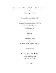
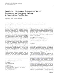
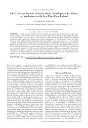
Scattering1 Classical scattering of a charged particle (RutherfordScattering)Begin by considering radiation when charged particles collide. To find the radiation, werequire the acceleration of the interacting charges, which means we need the particle trajectoriesas they move subject to the Coulomb potential. Note that we are neglecting the factthat radiation results in energy loss and therefore trajectories change due to energy loss in thescattering. The classical scattering equation for this porcess is called Rutherford scattering,although the equation for the particle trajectory also describes the motion of any 2 particlesinteracting via a 1/r potential (eg bound states or even particles interacting gravitationally).The geometry is shown in figure 1. Here we ignore the motion of the heavier particle, or weuse CM coordinates. (That is, we assume a fixed scattering center.)ImpactParameterClosest ApproachxdΩSolid AnglesθzyFigure 1: Motion of a particle in a central (1/r) potnetial.The incident angular momentum is L = mvs = s √ 2mT 0 , where m is the projectile mass,v its velocity, s its impact parameter, and T 0 its initial energy at at time t = −∞. LetI equal the number of particles per unit area per second (incident flux). The number ofparticles in the ring between s and s + ds are scattered into the ring between θ and θ + dθ.The definition of the cross section for scattering, σ, is the number of particles scattered persecond divided by the incident flux. The cross section has units of area. In this case, thedifferential cross section is obtained by the following equation representing the fact that thenumber incident in the ring defined by the impact parameter, s, equals the number scatteredinto the ring defined by the solid angle, d Ω.[I 2πs ds] = −2π sin(θ) dθ [I dσdΩ ]Therefore the differential cross section is obtained by dividing by sin(θ) dθ. The negativesign notes that as s increases the angle θ decreases.1

dσdΩ = − sin(θ) sdθdsAssuming a completely elastic collision, energy is conserved during the motion of the charge.Thus in spherical coordinates, the conservation of energy is given by;(1/2)mṙ 2 + (1/2) L2mr 2 + U = constant = T 0The angular momentum, l for a central force (Coulomb) is also conserved. This is;l = mr 2 ωThis allows an exchange of the variable of integration from t to θ.dθ ′ =l drmr 2√ (2/m)[t 0 − U r − l 2 /(2mr 2 )]This is integrated after using the Coulomb potential, U =4πǫ 1 zZe2 r . Here z and Z are thecharge on the particle and scattering center, respectively, and e the electronic charge. Thesolution is;(1/r) = − mqQL 2 (1 + η cos(θ) ′ )This is the equation of a hyperbola or an ellipse depending on the sign of the energy. Theexcentricity, η, is√η = 1 + 8πǫE 0L 2mzZ(e) 2Now Change the angle θ ′ to the scattering angle θ as observed in Figure 2, where θ = π−2θ ′ .This results in the equation;cot(θ/2) = 8πǫT 0szZe 2s = zZe28πǫT 0cot(θ/2)Substitution into the equation for the cross section gives;dσdΩ = [ zZe24πǫT 0] 2 [ 1sin 4 (θ/2) ]In reality the scattering is not elastic as the charge is accelerated and loses energy. Thisloss could be determined by a perturbation series as it is small. However, to first order thetrajectory does not change so the velocity and acceleration of the charge q can be foundusing the acceleration as determined from the equation of motion to get the radiated power.2

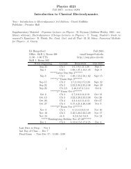
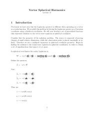
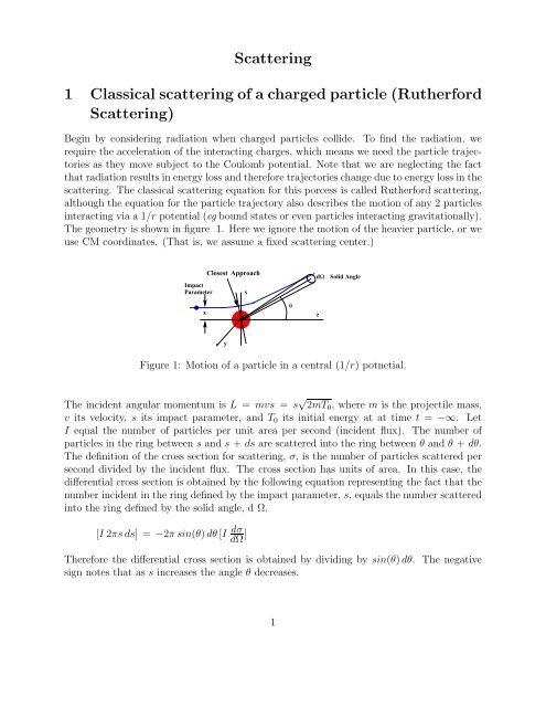
sClosestApproachθxθθFigure 2: The geometry to convert the angle used to solve the equation of motion to thescattering angle2 Solution to the scattering equationIn the above section we considered scattering of a particle from another particle when theinteraction between them was the Coulomb force (represented as will be seen later, bythe exchange of a virtual photon). In this section we develop a general description of thescattering of a classical, real photon from a charge.This scattering can be considered as a solution to the wave equation. Although we will usethe scalar wave equation, recognize that a vector such as an EM field can be considered asa set of scalar components. The wave equation has the form;[∇ 2 − (1/c 2 ) ∂2∂t 2 ]ψ = S(⃗r, t)In the above, ψ is the wave amplitude and S the scattering center, or in this case the sourceof the scattered wave. In the case of EM scattering, the source of the scattered wave dependson the strength of the incident wave so we rewrite this term as S → Sψ. In the scatteringregion (ie as r → ∞) the solution, ψ, consists of an incident wave plus an outgoing sphericalwave. Scattering assumes that the the source term is localized so that sufficiently far awaythis term → 0 and waves in this region are solutions to the homogeneous wave equation.Now we also assume that the source ands solution are harmonic in time, ψ(⃗r, t) → ψ(⃗r)e iωtwhich removes the time dependence of the equation. The full wave equation is then;[∇ 2 − k 2 ]ψ = S(⃗r)ψThe incident wave has the form of a plane wave solution;3

ψ in = e ikz = e ikr cos(θ) .The scattered wave has the form of an outgoing spherical wave;ψ out → f(θ, φ) eikrrThen the asymptotic form of the solution as r → ∞ of the scattering equation isψ = ψ in + ψ outwith R = |⃗r −⃗r ′ | and L operating on the wave amplitude, ψ, which equals the source. Thenif we formally define an operator L −1 . The solution we seek has the form at a time t → ∞;ψ = ψ in + ψ outwhere ψ in is the form of the incoming wave and ψ out is the outgoing spherical wave. Thewave equation can be written in operator form as;ψ out = L −1 Sψ.Formally we can then write;ψ out =11 − (L −1 S) L−1 (Sψ in )Then substitute for ψ = ψ in + ψ out and collect terms. The formally solution is then writtenas;ψ out = [1 + L −1 S + L −1 SL −1 S + · · ·] ψ inThe series converges if the source term is sufficiently small. Generaly the scattered EM waveis much less than the incident wave so we take the first term, called the Born term, as theapproximate solution. The differential scattering cross section is then defined by the scatteredpower into a solid angle dω divided by the incident flux. The incident flux is obtainedfrom the Poynting vector of the incident plane wave.S in = |E| 2 /µcThus the cross section in the Born approximation can be written;dσdΩ=(1/cµ)|f(θ, φ)|2(1/cµ)|e ikz | 2 = |f(θ, φ)| 2 4

Now a properly normalized outgoing Green’s function for a point source can be written ase ikRR(ie the Green function in a previous lecture). Therefore the solution in practical ratherthan in the above formal formal terms can be written ;ψ out = ∫ d⃗r eikRR S(⃗r′ )ψ in + ∫ d⃗r eikRR S(⃗r′ )ψ outThis is not a solution but an integral equation because ψ is not known until the solution isobtained, ie the source term in the intergand is unknown.3 Scattering of the EM waveScattering generally occurs when the EM wavelength is large compared to the scatteringsource. EM Scattering occurs when some of the incident wave is absorbed and re-radiated.As in radiation, we keep the lowest terms in the multipole expansion of the scattered fields.Almost always this results in dipole radiation as the incident wave polarizes the charges inthe scattering center. If the incident wave has large amplitude, then it is possible that thecharges will not move linearly with the incident E field, but will bend due to the ⃗v × ⃗ B forceof the magnetic component in the incident wave. An intense incident wave would probablyalso require terms of higher order than the Born term in the perturbation expansion forthe cross section. The scattering formulation occurs as follows (we always assume a timedependence of e iωt )A plane, monochromatic, linearly polarized wave is incident on a scattering center. Theincident wave is polarized in the ˆx direction and moves in the ẑ direction.;⃗E in = ˆxE 0 e ik inrcos(θ)⃗B in = ˆk in /c × ⃗ E inThese fields induce dipole moments (⃗p, ⃗m) in the scattering center. The dipoles radiate energy.This radiation can be calculated in the multipole approximation which uses the staticfields obtained from the multipole moments. The dipole fields are;⃗E sc =4πǫ k2 eikrr [ˆn × ⃗p × ˆn] − z 0k 24π eikrr [ˆn × ⃗m]⃗B sc = (1/c)ˆn × ⃗ E scIn the above, ⃗p and ⃗m are the induced electric and magnetic dipole moments.5

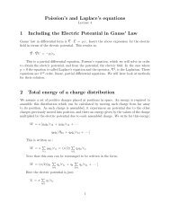
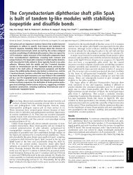
zθn^^k ina^xx^φa^yFigure 3: The geometry used to obtain the polarization vectors for scattering from a dielectricsphere4 Dipole cross section for a dielectric sphereUsing the Poynting vector and the dipole fields obtained previously. We find the differentialradiated power for dipole.dσdΩ = r2 |â · ⃗E sc | 2ẑ · | E ⃗ in | 2The unit vector â defines directions perpendicular to the observation direction ˆn. Substitutionfor the field givesdσdΩ =k4(4πǫ) 2 |â · ⃗p + (1/c)(ˆn × â) · ⃗m| 2For a small dielectric sphere of radius, η, the electric dipole moment of the sphere is;⃗p = 4πǫ 0 ( ǫ − 1ǫ + 2 )η3 ⃗ EinUse the geometry shown in Figure. 3. The cross section is obtained for the scattered polarizationperpendicular â ⊥ and parallel, â ‖ to the scattering plane as defined by the planecontaining the incident and scattering vector directions. From the figure;â ‖ · ˆx = cos(θ) cos(φ)â ⊥ · ˆx = −sin(φ)Averaging over all possible initial polarizations (ie averaging over φ) we obtaindσ ‖dΩ = k4 η 62 |ǫ − 1ǫ + 2 |2 cos 2 (θ)6

dσ ⊥dΩ = k4 η 62 |ǫ − 1ǫ + 2 |2The total differential cross section is;dσdΩ = dσ ‖dΩ + dσ ⊥dΩThe total cross section is obtained by integration over dΩ.σ T = 8πk4 η 63| ǫ − 1ǫ + 2 |2The polarization of the scattered wave is;P(θ) = dσ ⊥/dΩ − dσ ‖ /dΩdσ ⊥ /dΩ + dσ ‖ /dΩ =sin2 (θ)1 + cos 2 (θ)5 Form factorSuppose the scatterers are a system of charges with fixed locations in space. The resultis a superposition of scattering amplitudes from all the point scattering centers. We havepreviously seen that coherence must be included when one adds the contributions from eachscattering point. Assume that the positions of the scatters are located by the vectors, ⃗x j .The incident wave will have the phase factor, e ik 0ˆn 0·⃗x j, and the phase for the scattered waveat large distances will be e ikˆn·⃗x j. Here ˆn 0 is the direction of the scattered wave. We assumedipole scattering and write;dσdΩ =k4(4πǫ) 2 | ∑ j[â · ⃗p j + (1/c)(ˆn × â) · ⃗m j ] e i⃗q·⃗x j| 2In the above write ⃗q = kˆn 0 − kˆn = k(ˆn 0 − ˆn) for elastic scattering from massive points,(ie no recoil). Then suppose that the scatterers are identical so that ⃗p j = ⃗p and ⃗m j = ⃗m.Rewrite the above as;where;dσdΩ = [dσ sdΩ ] F(q)dσ sdΩ =F(q) = | ∑ jk4(4πǫ) 2 [â · ⃗p j + (1/c)(ˆn × â) · ⃗m j ] 2e i⃗q·⃗x j| 2 = ∑ jne i⃗q·(⃗x j−⃗x n)7

For a random distribution of a large number of scattering centers the phase difference betweenthe points causes the structure factor,F(q), to average to zero unless j = n. Whenj = n, the sum results in F(q) = N, the number of scattering centers. On the other handif the scattering centers are distributed in an ordered array then F(q) is small unless ⃗q ≈ 0.This is coherent scattering. Thus consider the form in 1-D;∑e i⃗q·(⃗x j−⃗x n) → ∑ e iqx je iqxnjnjnNow let x j = jd where d is the spacing of the centers. The sum is converted to an integral by;1 = [(j + 1) − j] = (δj) = [x j+1 − x j ]/d = ∆x/d∞∑j=−∞e iqx k =∑ (δj)eiqx k = (1/d)∞∫−∞dxe iqx k=δ(q)2πdFinally suppose the centers are distributed by some function f(⃗r) so that ⃗pf(⃗r) representsthe electric dipole moment per unit volume (use the electric moment here but it is obvioushow to include the magnetic moment). The scattering due to this distribution is ;dσdΩ =k4(4πǫ) 2 | ∫ d 3 x ′ (â · ⃗p) f(⃗r ′ ) e i⃗q·⃗x′ | 2which we re-write as previously;anddσ sdΩ =k4(4πǫ) 2 |[â · ⃗p] 2F(q) = | ∫ d 3 x ′ f(⃗r ′ )e i⃗q·⃗x′ | 2dσdΩ = dσ sdΩ F(q)The structure function (form factor) is the Fourier transform of the spatial distribution ofthe scattering centers.6 Expansion of a plane wave in spherical harmonicsThe scattering problem is solved naturally in spherical coordinates, as the center of the coordiantesystem is chosen to lie at the center of the scatttering source. Also the scatteringsolution is to be obtained in a multipole series as the scattering amplitude is observed as thedistance from the scattering center → ∞. However, a plane wave incident on the scatteringcenter is formulated in Cartesian coordinates. Thus we must formulate the incident wave in8

a spherical system, written in terms of spherical harmonics. We write;e ikz = e ikr cos(θ) = ∑ C n Y 0 nUse the orthonormal properties of the spherical harmonic to write;C n = 2π ∫ d(cos(θ)) Y 0 neikrcos(θ)Note that an integral representation of the spherical Bessel function, j l (kr), isj l (kr) = (−i) l /2π∫0d(cos(θ)) e ikr cos(θ) P n (cos(θ)We may also use the addition theorem which has the form;P l (cos(θ)) =4π2l + 1∑mYlm (θ 1 , φ 1 ) Yl ∗ m (θ 2 , φ 2 )where the angles (1) and (2) refer to the angles of vectors ⃗ k and ⃗r in the specified coordinatesystem. This gives the required form for the plane wave;e ikr cos(θ) = 4π ∑ i l j l (kr) Yl m (ˆk) Yl∗ m (ˆr)l,mThis form for the incident wave can then be matched at the scattering surface to the fieldequations inside and outside the scattering center by matching the boundary conditions atthe surface. Recall that a similar technique was used to obtain the reflection (scattering)and transmission coefficients of an EM wave incident on a dielectric and conducting surfaceplaner surfaces. For example, this technique can be used to develop Mie scattering (lightscattering from small dielectric particles).7 Thompson scattering (e.g.Classical EM scattering fromatomic electrons)The power radiated by an accelerated charge is obtained from the Poynting vector.⃗S = ⃗ E × ⃗ H = ǫc|E| 2 ˆnThe radiation field of an accelerated charge when β ≪ c is ;⃗E =4πǫ q × ˆn ×⃗˙β[ˆnR] ret9

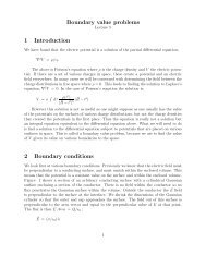
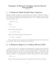
Thus the radiated power into solid angle dΩ is ;dPdΩ=q216π 2 ǫc [ˆn × ˆn × ⃗˙β] 2If a charged particle is accelerated by the ⃗ E field of an EM wave we have;⃗E I = E 0I e i(⃗ k·⃗r − ωt) ⃗η 0⃗F(force) = m⃗a = mc ⃗˙β = q ⃗ EI⃗˙β = (q/mc)E 0I e i(⃗ k·⃗r−ωt) ˆη 0Ignore phase differences (take the instantaneous time) and let (ˆη be the polarization direction,Figure 4.〈 dPdΩ 〉 = c ǫ ( q 24πmc 2 ) 2 |ˆη · ˆη 0 | 2The incident flux is the time-averaged Poynting vector of the incident wave so the crosssection is;dσdΩ = 〈(dP/dΩ)〉〈S in 〉dσdΩ = ( q 24πǫmc 2 ) 2 |ˆη · ˆη 0 | 2The evaluation of the factor |ˆη · ˆη 0 | 2 is obtained from Figure 4.ˆη 1 = cos(θ)[ˆxcos(φ) + ŷ sin(φ)] − ẑ sin(θ)ˆη 2 = −ˆx sin(φ) + ŷ cos(φ)Choose ˆη 0 = ˆx and sum over the final polarizations to obtain;|ˆη · ˆη 0 | 2 = cos 2 (θ) cos 2 (φ) + sin 2 (φ)This result can be substiuted above to obtain the scattered differential power. Note we haveneglected the effect of the magnetic field on the motion of the accelerated charge, but thiseffect was worked out to first order in an earlier example.10

IncidentDirectionzθn^ScatteredDirection^η 0xφθη^η^φ 21yFigure 4: The geometry used to evaluate the angles in Thompson scattering8 BremsstrahlungThe general form of the radiated energy,dWdΩ= ∫ dt dPdΩ ;Thus use ⃗ S = ǫc|E| 2ˆn and ⃗ E =dWdΩ= A ∫ dt |E| 2 R 24πǫ q × ˆn ×⃗˙β[ˆnR] Ret and write;In the above A is a constant depending on the charge. Take the Fourier transform of thefield using the time dependence of the field, e iωt .E(ω) = 1 √2π∫dt E(t) eiωtE(t) = 1 √2π∫dω E(ω) e−iωtThen substitute to obtain;dWdΩ= (AR 2 /2π) ∫ dt ∫ dω ∫ dω ′ E ∗ (ω ′ ) E(ω) e i(ω−ω′ )tdWdΩ= (AR 2 /2π) ∫ dω |E(ω)| 2Therefore we identify the frequency spectrum of the radiation where I is the intensity(power/area) as;d 2 IdωdΩ = 2A|E(ω)|2 R 2Now substitute for the radiation field of an accelerated particle (use the relativistically correctexpression);11

d 2 IdωdΩ = [ q 2 ∞∫16π 3 cǫ ]|−∞dt [ˆn × [(ˆn − ⃗ β) × ˙⃗ β](1 − ⃗ β · ˆn) 2 e iω[t−⃗ β·R/c] | 2For low frequencies, the exponential term is ≈ 1. Note that;ˆn × (ˆn − ⃗ β) × ˙⃗ β1 − ⃗ β · ˆn= d dtIntegrate by parts to obtain;d 2 IdωdΩ = [ q 2 ∞∫16π 3 cǫ ]|−∞d] [ˆn × ˆn × β ⃗1 − β ⃗ · ˆn[ˆn × ˆn × ⃗ β1 − ⃗ β · ˆnAlso assume non-relativistic motion, β → 0.d 2 IdωdΩ = [ q 216π 3 cǫ ]|ˆη · ∆⃗ β| 2]In the above ˆη is the polarization direction, and ∆ ⃗ β is the differential change in the velocityof the charge. In the soft photon limit, the energy of a photon is ω so the number of photonsinto dΩ and between frequencies between ω and ω + dω is approximately;q 2N ph = (1/ω)[16π 3 cǫ ]|ˆη · ∆⃗ β| 2The cross section for soft photon emission in a charged particle collision is;d 3 σ = [N dσdΩ q d(ω)dΩ ph ]gam dΩ qWhere dσdΩ qis the cross section for a Coulomb interaction (Rutherford scattering). Thensubstitute the various equations and integrate. Use figure 5 to obtain ∆ ⃗ β. The result forlow frequencies and non-relativistic motion is;dIdω =q24π 2 cv [ln(1.123γv wb min)]MvMvθQ = |Pin − Pout| < 2Mv∆ P ~ QFigure 5: The geometry for the momentum transfer12

q/2vvq/2φ oFigure 6: Radiation from sets of charge rotating in a circle∆ρ ∆p ≈ with ∆ρ = bb min (cut off value due to screening) = /2Mv = /Q max9 Radiation and coherenceWe have seen that an accelerated charge radiates energy. Suppose we set 2 charges in symmetricpositions on a loop and let them spin around the z axis as shown in figure 6. Thisresults in radiation because the charges are accelerated. Now suppose we consider the loopfilled with a continuium charge distribution that rotates. Contrary to intuition, there isno radiation. This occurs because of coherence of the radiation from each of the elementalcharge distributions cancels the radiation field. We see this as follows. The charge distributionof the two elements as shown in the figure can be written;δ(r − a)ρ = (q/2)a 2 δ(θ − π/2)[δ(φ + φ 0 ) + δ(φ − φ 0 )]We rewrite the charge per unit length so that we can add additional symmetric units ofcharge;λ =q(n + 1) πa δ(φ − πk/N − φ 0) k = 0, 1, 2, · · · , N − 1All of the charge elements rotate with the frequence ω. The charge density is then written;ρ k =q δ(r − a)(n + 1)π a 2 δ(θ − π/2) δ(φ − πk/N − ωt)13

Now work out the Fourier components of the distribution.ρ k = ∑ A n cos(n[φ − ωt])The coefficients A n are found using othorgonality of the Fourier functions, so that;Then;ρ k =q δ(r − a)(n + 1)2π a 2 δ(θ − π/2) ∑ ncos(2πkn/N) cos(n[φ − ωt])ρ = N−1 ∑k=0ρ kThe sum over k provides the followingN−1 ∑k=0cos(2πnk/N) = cos(nπ[1 − 1/N])sin(nπ)sin(nπ/N)This is zero unless n = N or 0. Thus the radiation has multipolarity N. But if N → ∞there will be no radiation. In effect the radiation from each charge elecment contributescoherently, cancelling the radiated power.10 Index of refractionWe choose to look at a simple model that will demonstrate that the index of refraction isdue to an interference between the incident wave and the scattered wave represented byradiation from absorption of the incident wave on atomic electrons. Look at fig 7. Theatomic electrons in a ring of radius ρ in the (x, y) plane are caused to harmonically oscillatedue to a plane wave incident along the z axis. We assume the electric vector of this wave ispolarized in the x direction.The electrons are bound to atoms, we assume by a linear force, resulting in the non-relativisticharmonic force equation;m d2 xdt 2 + kx = qE e iωtThe 1 2t term is the intertial force, ma, the 2 nd term is the restoring force keeping the electronbound to the nucleus, and the 3 rd term is the driving force due to the EM field.The solution is ;x = x 0 e iωt = qE/mω 2 0 − ω 2 e iωt 14

xEρyrPzFigure 7: A schematic of a model for an incident plane wave scattered from a ring of atomicelectrons in the x, y) planeThe time derivatives give the velocity and acceleration which are placed in the non-relativisticexpression for the radiation field.E = (e/4πǫ)[ˆn × ˆn × ˙⃗ β] e iωt /rNow multiply by the number of electrons per unit area in the plane, N, and integrate overthe surface of the plane 2π ∫ ρ dρ. Change the variable to an integration over the distancefrom the electron to the observation point on the z axis, r 2 = ρ 2 + z 2 and approximate thevalue of t ′ as t ′ ≈ t − r/c. This results in the expression;E total = qN4πǫcE total = 2πqNω2 x 04πǫcE total ≈ 2πiqNωx 04πǫc∫ρ dρ∫dφ ω 2 x 0 e i(ωt−R/c)e iωt ∞ ∫ze iω(t−r/c)rdr e −iωr/c /rTo this result we add the incident wave e iω(t−z/c) . Now we can write the wave at the pointz as due to a wave having the form,E = E 0 e iω(t−(n−1)∆z/c−z/c)The incident wave propagation from the plane is just e iω(t−z/c) the additional term (n−1)∆z/cis the time delay experienced by the wave when passing through the dielectric material havingindex n and thichmess, ∆z. For small values of ∆z expand this term to write the fieldat the observation point as;15

E ≈ E 0 e iω(t−z/c) iω(n − 1)∆z[1 − c ]Divide through by the thickness ∆z and identify this result with the previous calculation ofthe scattered field;(n − 1) = 2πq2 (N/∆z)4πǫm(ω 2 0 − ω2 )The term N/∆z is the Number density of the electrons.11 Cherenkov RadiationCherenkov radiation occurs when a charged particle is moving faster that EM radiation travelsin that medium. Observe figure 8. The present point lies a further distance from theretarded point than the observation point. That is V (t − t ′ ) > (c/n)(t − t ′ ). Here, n is theindex of refraction of the medium. A wave front can be drawn as a line that lies from thetangent to the spherical wave front to the present point as shown in fig. 8. Each sphericalwave front from a point along the particle trajectory will be tangent to this line. The angleof propagation of the wave front θ is obtained from the figure as;(c/n)tθFigure 8: The geometry of wave fronts in Chernekov radiationvtcos(θ) = ct/nvt= 1nβPreviously we chose the retarded point of the Lienard-Eiechert potentials because of causality.In Cherenkov radiation both retarded and advanced points are possible solutions as onecan see in fig. 9 The positions of the observation and present points are related by (we usec here but note that it is really c/n);c(t − t ′ ) = | ⃗ X + ⃗ V (t − t ′ )| = R/c16

RetardedPointn^R =c(t − t’)θβObservationPointR XAdvancedPointV(t − t’)αPresentPointFigure 9: The geometry of Chernekov radiation showing the retarded, advanced, and observationpointsThis equation is written for ∆t = (t − t ′ ) ;c 2 ∆t 2 = X 2 + V 2 ∆t 2 + 2 ⃗ X · ⃗V ∆t.This is a quadratic equation with solutions;√∆t = − X ⃗ · ⃗V ± ( X ⃗ · ⃗V ) 2 − (V 2 − c 2 )X 2(V 2 − c 2 )We have that ∆t > 0 so that there is only one real positive root for V < c which correspondsto the retarded point. For V > C there is no real root for ⃗ X · ⃗V > 0 but when ⃗ X · ⃗V < 0there are 2 solutions. This occurs for values of α > π/2 . From the discriminate;cos(α) = −[1 − (c/v) 2 ] 1/2These solutions are the advanced and retarded points, so the Lienard-Wiechart potentialscan be simply multiplied by 2 to include the advanced point as both retarded and advancedpoints are a distance X away from the observation point.Now we look more carefully at this solution which represents a shock front singularity. Thegeneral form of the angular distribution of the radiated power is written;dPdΩ= (1/2µc)Re| ⃗ E ∗ · ⃗E|R 2We develop the Fourier spectrum of the E field, by;17

E = √ 1 ∞∫2π−∞E(t) = √ 1 ∞∫2πdt e iωt E(t)−∞dt e −iωt EThe energy radiated is the time integral of the power. Therefore;dWdΩ= 12πµc∞∫−∞dt∞∫−∞dω∞∫−∞dω ′ ⃗ E∗ · ⃗E e i(ω′ −ω)tInterchange the time and frequency integration and differentiate with respect to ω.dWdΩ= 12µc |E(ω)|2 R 2The above is the energy radiated per unit solid angle. The equation has been multiplied bythe differential area element, R 2 dΩ and a factor of (1/2) is included so that we define ω > 0always. The radiation field (Gaussian units) is;E(t) = (q/c)[ ˆN × (ˆn − β) ⃗ × ˙⃗ βκ 3 ] = (e/cκ) d Rdt [ˆn × (ˆn × β)] ⃗The right side of the energy equation has the form G ∗ G.G = 1(4µc) 1/2 E(ω)R = 1(8πµc) 1/2∞∫−∞dt e iωt [ˆn × (ˆn − ⃗ β) × ˙⃗ βκ 3 ]Change to present time units, κt, and approximate the time in the phase component byt ′ ≈ t − ˆn · ⃗r/c for large r. Integrate by parts over the time, and then put this value for Gback into the equation for the differential power above to obtain;d 2 Idω dΩ = q2 ω 216π 2 c 3 |∞∫−∞dt[ˆn × (ˆn × ⃗ β)] e iω(t−ˆn·⃗r/c) | 2In a dielectric medium the velocity of the EM wave is c → c/n = c/ √ ǫ with n the index ofrefraction. Assume straight line motion so that ⃗r = ⃗ V t .d 2 Idω dΩ = µq2 cω 216π 2 |ˆn × V ⃗ ∞∫(ω 2 /2π) dt e iωt(1−ˆn·⃗r/nc) | 2−∞The integral is a δ function and results in the expression for the intensity of the Cherenkovradiation (Gaussian units);d 2 Idω dΩ = q2 β 2nc sin2 (θ)|δ(1 − (β/n) cos(θ)| 2The above δ function gives the Cherenkov angle as previously obtained. As an example,glass has an index of refraction of 1.5. The Cherenkov angle is then;18

cos(θ) = 1/(1.5β)and gives a cut-off velocity of β = 0.666 An electron with this velocity has a momentum of0.45 MeV.12 Synchrotron radiationSynchrotron radiation occurs when a particle is acclerated perpendicular to the velocity asin a circular orbit. It occurs naturally for electrons moving around the magentic field lines inthe upper atmosphere of the earth, and in electron accelerators used to produce EM radiationfor studies of material strucutre and biological samples. Suppose a relativistic particle in acircular orbit as shown in figure 10. The radius of the orbit is ρ, and we assume a pulsedbeam to avoid coherence because a uniform, continuious beam no radiation occurs.ψρρ2/γ BdAObserverRadiationconeθFigure 10: Synchrotron radiation beams from a circular acceleratorThe arc distance A to B is d = 2ρ/γ. The time for the particle to travel this distance ist = d/v. The first photon leaves the initial pulse from A and travels a distance t/c duringthis time interval. Thus the distance between the 1 st and last photon in the emission coneis ∆L;∆L = 2ργ [1/β − 1] ≈ ρ/γ3The time for the EM pulse to travel this distance is ρ/(γ 3 c) which determines the frequencycut-off for the radiation; ω c = γ 3 c/ρ . We obtain the radiated power from the expression forthe power per solid angle per frequency obtained in the Cherenkov radiation section;d 2 IdωdΩ = q2 ω 216π 2 c 3 |∞∫−∞dt[ˆn × (ˆn × ⃗ β)] e iω(t−ˆn·⃗r/c) | 219

zn^θyvtρxvρFigure 11: The geometry used for synchrotron radiation of an ultra-relativistic particleChoose a coordinate system as shown in fig. 11 and substitute for the velocity and the distancefrom the retarded point to the present point, rAlso;ˆn × (ˆn × ⃗ β) = βˆn × (ˆn × [ˆǫ parallel sin(vt/ρ) + ˆx cos(vt/ρ)])ˆn × (ˆn × ⃗ β) = β(−sin(vt/ρ) ˆǫ ‖ + cos(vt/ρ) sin(θ) ˆǫ ⊥ )ˆn · ⃗r = (ρ/c)sin(vt/ρ) cos(θ)Integration proceeds in the ultra-relativistic approximation, β ≈ 1. The result isd 2 Iω dΩ = 27 e2 c λ c32π 3 cρ λ γ8 [1 + (γψ) 2 ] 2 [K2/3 2 (η) +In this equationλ c = 4πργ−33η = λ c[1 + (γψ) 2 ] 3/22λK j i/2 are modified Bessel functions of the 2nd kind.(γψ)21 + (γψ) 2 K 2 1/3 (η)]13 Virtual photonA charged particle of momentum ⃗p I and energy E I cannot decay into a photon and a chargedparticle having the same mass. Such a process is shown in fig. 12. If we attempt of conserve20

oth energy and momentum, write;⃗p I = ⃗p F + ⃗p γE I = E F + E γWhen combining the equationsM 2 γ = E 2 γ − p 2 γ = 2[M 2 + p I p F cos(θ) − E I E F ]In the above M is the mass of the particle and θ is the angle between the incident andoutgoing momentum. Now M 2 γ < 0 so that M γ is imaginary. However, in some cases it isuseful to think that this photon has some of the the properties of a real photon. Indeed inQM such a virtual particle can live within the uncertainty relation ∆E ∆t ≈ . For laternotation we let this photon have energy ω = E I − E F and momentum ⃗q = ⃗ P I − ⃗p F . ThenM 2 γ = ω2 − q 2 < 014 Scattering of virtual quantaThis technique is an approximation to the interaction of charged particles, by viewing thefield as a collection of virtual photons. The approximation works for photons that are almost“on the mass shell”, ie virtual photons that have mass nearly zero.Consider the scattering of a charged particle from another charge system. The figure 12 isa schematic of the model to be described. Indeed the figure illustrates how bremsstrahlungcould be described as the scatering of a virtual photon into one of real mass. Generally wewould have a light particle scattering from a heavier one, but we use a frame in which theheavier mass is in motion and the lighter mass is at rest so that the motion of the heaviermass can be assumed to move with constant velocity during the collision. The lighterparticle recoils and emitts radiation. The relativistic factor for the movement of the chargeQ is γ ≫ 1. Now if γ ≫ 1 the E and B fields are almost transverse. The fields at point P are;E 1 = Q4πǫE 2 = Q4πǫγvt(b 2 + (γvt) 2 ) 3/2γb(b 2 + (γvt) 2 ) 3/2⃗B = ⃗ V × ⃗ EThe equation for the ⃗ B is due to the fact there is no magnetic field in the rest frame of Q.The E field is just the static field of a charge Q a distance r ′ away from the point, Q. Apply21

QRecoilqVirtualGammaRealGammaFigure 12: A schematic of the scatteing of a photon from the field of a charge Qx2(−vt,b,0)QVx2’S2x1x3x1’Px3’S1Figure 13: The geometry uses for calculating the EM impulse due to the EM fielda Fourier transform to the wave equations for the vector and scalar potentials;[k 2 − ω 2 /c]V (k, ω) = (−1/ǫ)ρ(k, ω)[k 2 − ω 2 /c] ⃗ A(k, ω) = (−µ) ⃗ J(k, ω)Then let ρ = Qδ(⃗x − ⃗ V t) and ⃗ J = ⃗ V ρ. Apply a Fourier transform to obtainρ = Q 2π δ(ω − ⃗ k · ⃗v)The potentials then have the form;V = −2πǫQ δ(ω − ⃗ k · ⃗v)k 2 − ω 2 /c 2⃗A = ⃗v/c 2 VThe fields are then obtained from ⃗ E = ⃗ ∇V − ∂ ⃗ A∂tand ⃗ B = ⃗ ∇ × ⃗ AThis results in;⃗E( ⃗ k, ω) = i(ω⃗v/c 2 − ⃗ k)V22

⃗B(k, ω) = i/c 2 ( ⃗ k × ⃗v)VTo get the fields at a distance perpendicular b to the particle path;⃗E(b, ω) =Integration gives1(2π) 3/2 ∫d 3 k ⃗ E(k, ω)e ikxbE z (ω) = − iωQ √2/π(1 − βV 2 2 )K 0 (λb)ǫE x (ω) = Q √2/π (λ/ǫ)v 2 K1 (λb)ǫwhere λ = (ω 2 /v)[1 −β 2 ], and K i are modified Bessel functions. The fileds have a spectrumof frequencies. We can calculate a Poynting vector;⃗S = (1/µ) ⃗ E × ⃗ BThis can be written in terms of the Fourier transforms of E and B as ;W/Area =∞∫−∞dω E(ω) B ∗ (ω)However the frequencies for E and B must be the same, ie time correlated. This is true forE 2 and B 3 which gives an electromagnetic pulse of photons in the S 1 direction. However,E 1 and B 3 are not. We arbitrarily add a magnetic field so that ⃗ B 3 → [B 3 + E 1 ]ˆx 3 . Thisgenerates a pulse S 2 . Note that this B field has no effect on the static problem and in anyevent the pulse S 1 dominates the impulse.There are then two photon flux terms;⎛ ⎞d 2 I 1(⎝ dω d area ⎠ Qd 2 =2 c (ωb/γv) 2 K 1 (ωb/γb)I 2 4π 3 ǫv 2 b 2 (ωb/γv) 2 K 0 (ωb/γb)dω d areaThen integrate over the impact parameters;dI∞∫dω = 2π bdbd 2 I 1dω d areab minIn the above the total value of the Power spectrum I 1 + I 2 is used. This results in;dIdω = Q2 c2π 2 ǫv [χ K 0(χ) K 1 (χ) − (β 2 /2)χ 2 [K1(χ) 2 − K0(χ)]]2)23

with χ = ωb minγv . The minimum impact parameter can be obtained from the uncertaintyrelation b min q max = with q max = | P ⃗ I − ⃗p F |dσdΩ = ( q 2(4π) 2 ǫmc 2 ) 2 [1/2(1 + cos 2 (θ))]24