analysis of temperature and pressure characteristics ... - Orkustofnun

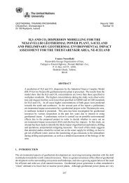
GEOTHERMAL TRAINING PROGRAMME Reports 2010Orkustofnun, Grensásvegur 9, Number 6IS-108 Reykjavík, IcelandANALYSIS OF TEMPERATURE AND PRESSURECHARACTERISTICS OF THE HVERAHLÍD GEOTHERMAL FIELDIN THE HENGILL GEOTHERMAL SYSTEM, SW-ICELANDMisghina Afeworki OkbatsionMinistry of Energy and MinesDepartment of Mines213 Liberty Avenue, Asmara, P.O. Box 272ERITREAmsgn_afe@yahoo.comABSTRACTThe Hverahlíd geothermal field is a high-temperature field located in the southernpart of the Hengill geothermal system. Interglacial lava series dominate thegeological succession at Hverahlíd with subordinate sub glacial hyaloclastites.Very active northeast trending fissure swarms with northwest trending transformstructures are believed to supply the main permeability for geothermal fluid flow inthe area. Analysis of temperature and pressure profiles from four boreholes revealsthe presence of three major feed zones at 800, 1000-1200 and 1800-2000 m depths.The reservoir at Hverahlíd geothermal field is characterised by formationtemperatures of more than 300°C and pressures well over 85 bars at the best feedzones. The main up-flow zone is located in the middle of the area with a northwestdirected lateral flow. A homogenous reservoir model with constant pressureboundaries fits best in simulating the injection well tests of three boreholes inHverahlíd. The reservoir is characterised by high transmissivity and storativityvalues; injectivity index values comparable to the average values in the Hellisheidiarea were obtained.1. INTRODUCTIONThis paper is written in partial fulfilment of the requirements of the six months geothermal trainingprogramme in UNU/GTP-2010. The report discusses the main findings and outcomes of temperatureand pressure data analysis of the geothermal system at Hverahlíd, Hengill area, SW-Iceland.Iceland is an island located in the northern part of the Atlantic Ocean. The country is situated in themiddle of the Atlantic Ocean and resides on top of the northern Mid-Atlantic Ridge. The Mid-AtlanticRidge is a divergent plate boundary and marks the locus of points along which the North Americanplate and the Eurasian plate are drifting away from each other in the northern part of the AtlanticOcean. These plates are diverging at a relative motion of 2 cm/year (Björnsson, 2004). Iceland isformed as a result of extensive volcanism along this ridge and offers the only sub-aerial exposure ofthe ridge. Enhanced magmatic and tectonic activity in the Icelandic crust combined with richgroundwater resources from glaciers and hydrologic circulations present a unique combination ofcriteria for the remarkable abundance of geothermal resources in the country.1

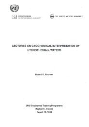
Misghina Afeworki 2 Report 6Geologically Iceland can be divided into three zones based on the age of the basaltic rocks (Iceland onthe web, 2010). Tertiary flood basalts make up most of the northwest and east quadrant of the island.Quaternary flood basalts and hyaloclastites are exposed in the central and southwest parts of theisland. These Quaternary rocks are cut by distinct volcanic zones; areas of active rifting that containmost of the active volcanoes. Fissure swarms make up most of the volcanic zone. These volcaniczones comprise about one-third of the area of Iceland and it is mainly in these zones that most of thehigh-temperature geothermal systems reside. Three main active volcanic zones (Figure 1) have beenrecognized in Iceland: the south-western, eastern and northern volcanic zones (Níelsson andFranzson, 2010). The Hengill geothermal or volcanic system comprises the Hengill central volcanoand several geothermal fields like the Hellisheidi and Nesjavellir fields from where currently a total of330MWe is being produced (Árnason et al., 2010). This enormous geothermal system is part of thesouth-western volcanic zone. The main focus of this project, the Hverahlíd geothermal field, formsthe southern part of the Hengill geothermal system. The intention in this paper is to present acharacterisation of the geothermal reservoir in Hverahlíd based on analysis of temperature andpressure profiles measured in four boreholes (HE-21, HE-36, HE-53 and HE-54) and analysis ofseveral injection well tests conducted in three of these boreholes (HE-36, HE-53 and HE-54).RR=Reykjanes RidgeRP=Reykjanes PeninsulaVI = Vestman IslandsSISZ=South IcelnadSeismic ZoneWVZ=Western Volcanic ZoneEVZ=Eastern Volcanic ZoneMVZ=Mid Iceland Volcanic ZoneNVZ=Northern Volcanic ZoneTFZ = Tjörnes Fracture ZoneFIGURE 1: A simplified tectonic map of Iceland; orange circle shows location ofthe Hengill geothermal system, red/dark dots indicate high-temperature areas andwhite areas are glaciers (modified from Hardarson et al., 2010)1.1 Organization of the reportIn this paper a step by step insight is given into the different aspects of the Hverahlíd geothermal field.In Section 2 the focus is on describing the geology of Hverahlíd geothermal field, in association with abrief description of the geology of the Hengill geothermal system to provide a broader perspective ofthe geology in the area. Furthermore, some geophysical studies conducted in the area are introduced.These are intended to provide an insight into the preliminary geological model of the geothermalsystem.In Section 3, the geothermal reservoir is analysed by means of different temperature and pressuremeasurements and profiles. An interpretation of the temperature and pressure profiles from fourboreholes shows the different feed zones present in the wells. Based on these profiles an attempt wasalso made to give an estimate of the formation temperature and pressures in the four boreholes. Twodimensionalcross-sections to show the distribution of temperature and pressure in the geothermalreservoir are presented. This is aimed at providing better visualization of the flow patterns, up-flow

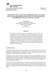
Report 6 3 Misghina Afeworkizones and cooling zones in the geothermal reservoir. Section 4 presents a description of severalparameters resulting from well test analysis. A number of injection tests were done in all of theboreholes at Hverahlíd. ISOR’s WellTester software (Júlíusson et al., 2008) was used to analyse theinjection tests and various pressure and reservoir models are discussed. Section 5 deals withproduction well testing by giving a brief discussion of the theoretical background of production welltesting and a description of the characteristic well curves that were drawn by Reykjavik Energy(Sigfússon et al., 2010). Finally the report presents the conclusions drawn and a summary of theoutcomes of all the data analyses done.1.2 Location and description of the study areaThe Hverahlíd high-temperature geothermal fieldis located in the southwest part of Iceland, in thesouthern part of the Hengill geothermal system(Figure 2). Hverahlíd is located about 30 km eastof Reykjavik, the capital. The area ischaracterised by gently rolling grassy or rockyplains bound by the fault scraps of the Hengillcentral volcano towards the west. Hengill is thehighest peak in the area rising above thesurrounding plains. The Hverahlíd area is easilyaccessible due to the fact that it is located nearone of the major highways in the country thatruns to the southern parts of Iceland. Two powerplants are already operated in the Hengillgeothermal system and a third one is planned atHverahlíd. The Nesjavellir power plant is locatednorth of Hengill (Figure 2) and the Hellisheidipower plant northwest of Hverahlíd. Both ofthese are electrical power stations and the formerone is operated as a combined power plant,producing both hot water for direct use, i.e. fordistrict heating, and electricity.2. BACKGROUNDFIGURE 2: Location map of Hverahlídgeothermal field and the Hengillgeothermal systemThis chapter focuses on describing the geology of the Hverahlíd geothermal area, in association with abrief description of the geology of the Hengill geothermal system. A brief review of surfacegeophysical studies conducted in the area is included as well to provide a broader perspective of thegeology in the area.2.1 Geology of Hverahlíd and the Hengill areaNíelsson and Franzson (2010) describe the Hengill area as being situated at a triple junction where twoactive rift zones (the Reykjanes Peninsula volcanic zone and the western volcanic zone) meet aseismically active transform zone (the South Iceland seismic zone). Figure 1 shows the differentvolcanic zones of Iceland with respect to the Hengill geothermal system. The dominant rockformations in the Hengill area are subglacial hyaloclastites (tuffs, breccias and pillow lavas). Lavasuccessions from interglacial periods flow to the lowlands and are therefore less common in the area(Helgadóttir et al., 2010; Níelsson and Franzson, 2010). The Hengill system is dominated by NE-SW

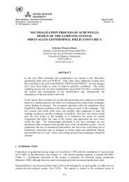
Misghina Afeworki 4 Report 6striking major fractures and faults. In some places, however, the fractures are intersected by easterlystriking features that possibly affect the permeability of the Hellisheidi field (Hardarson et al., 2010).Volcanic fissures of 9, 5 and 2 thousand years seem to play an important role as major outflow zonesin the field (Saemundsson, 1995; Björnsson, 2004; Franzson et al., 2005; and Franzson et al., 2010).The geothermal activity at the Hengill central volcano and its fissure swarms is explained by one ormore up-flow zones underneath the Hengill volcano. The up-flow is caused by buoyancy as hotintrusions in the roots of the volcano heat up groundwater. This, on the other hand, also creates apressure-low deep under the volcano so fluids from the outer boundaries of the system recharge theup-flow (Franzson et al., 2010). These fissures have been one of the two main drilling targets in theHellisheidi field. Large NE-SW fault structures at the western boundary of the Hengill graben, withmore than 250 m total throw, have also been targeted. In addition they have also been used as targetsfor the reinjection wells of the area (Franzson et al., 2010, Hardarson et al., 2010).The lithology in the Hverahlíd high-temperature field is mainly composed of two rock types:hyaloclastites and lava series. The lava series are the dominant formations and were formed duringinterglacial periods (Helgadóttir et al., 2010; Níelsson and Franzson, 2010). This makes Hverahlídsomewhat different to the rest of the Hengill system and Níelsson and Franzson (2010) suggest that theHverahlíd field was outside the main volcanism of the central volcano during the glacial periods.There are two types of intrusive rocks in the Hverahlíd high-temperature system (Níelsson andFranzson, 2010): dominant fine-grained basalt intrusions and minor andesitic to rhyolitic intrusions.The fine-grained nature of the intrusions indicates that they are dykes and/or sills. The intrusions areinfrequent down to about 800 m b.s.l. but become more numerous at deeper levels. Below 1600 mb.s.l. the intrusive rocks become a more dominant part of the lithological succession. A geologicalmap cropped out from the geological map of Hengill and a modified cross-section are presented inFigure 3.AA'BB'Lava field (10,300 years) Pillow lavasCompound lavasLava field (5500 years)FIGURE 3: a) Geological map of the Hverahlíd geothermal field (modified from Saemundsson,1995); b) Cross-section along line A-A’ showing the geological successionat Hverahlíd (modified from Níelsson and Franzson, 2010)2.2 Surface geophysical studies in Hverahlíd and HengillThe surface geophysical studies for the Hverahlíd area were done in conjunction with the Hengillgeothermal system. The information regarding geophysical studies presented here is from the TEMand MT resistivity surveys done by Árnason et al. (2010). Figure 4a shows the resistivity structure ofHengill geothermal system at 850 m b.s.l. A joint inversion of TEM and MT data from 148 soundingsites in the Hengill area reveals a resistivity structure consisting of a shallow low-resistivity layer inthe uppermost 2 km, underlain by high resistivity. At greater depth, a second low-resistivity layer isobserved in most of the area, again underlain by higher resistivity. The depth to this second low-

Report 6 5 Misghina AfeworkiABFIGURE 4: a) Resistivity at 850 m below sea level according to recent TEM surveys. High resistivitybelow low resistivity (< 10 Ωm) is shown as crossed lines, geothermal manifestations as red/blackdots, fissures and faults as blue or brown/grey wavy lines (modified from Hardarson et al., 2010)b) Density of seismic epicentres from 1991 to 2001 and inferred transform tectonic lineaments –green/grey straight lines (modified from Árnason et al., 2010)resistivity layer varies over the Hengill area. It is seen at the shallowest depth (about 3 km) under andaround Mount Hengill. The nature of the upper low-resistivity layer is known by comparing resultsfrom MT and TEM soundings and borehole data; it reflects conductive hydrothermal alterationminerals formed at temperatures between 100 and 240°C. The nature of the deep conductive layer isnot as clear, but its high conductivity could be due to magmatic brines trapped in ductile intrusiverocks. A NW–SE oriented low-resistivity anomaly through Mount Hengill and southeast of it is alsoseen. This anomaly is about 3.5 km wide and extends from about 3–9 km depth. Farther to thesouthwest, another NW–SE oriented zone of low resistivity is observed at somewhat greater depth.The low-resistivity anomalies at depth correlate with relatively positive residual Bouguer gravity,implying higher density. The NW–SE oriented, low-resistivity anomaly at 3–9 km under and to thesoutheast of Mount Hengill is found where intense seismic activity associated with transform tectonicsoccurs (Figure 4b). Since no attenuation of S-waves is observed under the Hengill area, the deepconductors are believed to reflect hot, solidified intrusions that are heat sources for the geothermalsystem above.3. ANALYSIS OF TEMPERATURE AND PRESSURE PROFILES IN HVERAHLÍD3.1 Description of the boreholes drilled in HverahlídThis section presents an analysis of temperature and pressure profiles that were measured in fourboreholes (HE-21, HE-36, HE-53, and HE-54) in the Hverahlíd geothermal field. The locations andorientations of these 4 boreholes are shown in Figure 5 and information about the dimensions of thesefour boreholes is presented in Table 1 (depth values are measured borehole depths). All theinformation presented here was obtained from the individual drilling and well completion reports ofthe boreholes (Mortensen et al., 2006; Níelsson and Haraldsdóttir, 2008; Matthíasdóttir et al., 2010).

Misghina Afeworki 6 Report 6FIGURE 5: Locations and trajectories of boreholesin Hverahlíd field (background map fromSaemundsson, 1995)HE-21 was the first well drilled in theHverahlíd area. It is vertical, drilled directlyabove a seismically very active fissure zonethat is believed to be the feeder for the surfacemanifestations that are present some 200 msouth of the borehole (Níelsson and Franzson,2010). HE-54 is a directional well directed tothe southeast of HE-21. HE-36 is locatedabout 1 km west of HE-21 and is a directionalwell. It was targeted at exploring the presenceof a geothermal reservoir associated with theactive fissure swarm west of HE-21. It wasdirected to the northwest, so it intersects theNE-SW trending fissure swarm more or lessperpendicularly. HE-53 is another directionalwell at the same drill site as HE-36 but with asouth-southwesterly direction, so it is almostparallel to the fissure swarm.Boreholeno.TABLE 1: Overview of parameters for the 4 boreholes in Hverahlíd;depths are measured borehole depths with respect to the drill platformDrilleddepth(m)Casing diameterSurface cas. &sections 1 and 2(″)Slotted linerin section 3(″)Direction(from wellhead)CasingdepthWell head coordinates(X,Y,Z)HE-21 2050 21, 17, 12¼ 8½ Vertical 903 385379, 391644, 356HE-36 2808 21, 17, 12¼ 8½ NW 1104 384583, 391528, 353HE-53 2507 21, 17, 12¼ 8½ SSW 965 384593, 391536, 353HE-54 2436 21, 17, 12¼ 8½ SE 759 385379, 391644, 3563.2 Interpretation of temperature and pressure profilesNumerous temperature and pressure profiles were done in all four boreholes in Hverahlíd. Themeasurements were done at several stages of the drilling and after drilling with or without injection.These profiles are the main bases of the analysis presented in this chapter.The profiles are classified into two major categories, i.e. during drilling and after drilling or warm-upprofiles. Both have been used to identify the main feed zones and to analyse the flow characteristicsin the reservoir. However, only the warm-up profiles were used in estimation of formationtemperatures and initial pressures in the Hverahlíd geothermal field.The measured borehole depth of the directional wells was converted to true vertical depth for theanalysis of formation temperatures. This was done by projecting the measured depth into a verticalplane that hypothetically passes through the well heads of each directional borehole. Figure 6 presentsselected plots of all the temperature profiles for each borehole. The ground surface is taken as acommon reference point for all depth measurements in each borehole. Therefore, depth measurementsrelative to the drilling platform were initially corrected to become depth measurements relative to theground surface.

Report 6 7 Misghina Afeworkia0Temperature (°C)0 100 200 300b0Temperature (°C)0 100 200 300Measured borehole depth (m)50010001500200028-01-200606-02-200605-02-2006 Q=18L/s05-02-2006 Q=21L/s05-02-200615-03-200613-02-200615-02-2006 Q=65L/s30-03-200629-11-200613-08-200910-06-2010Measured borehole depth (m)500100015002000250009-09-200709-09-200725-09-200727-09-2007 Q=30l/s12-10-2007 Q=40l/s17-10-2007 Q=33l/s20-10-2007 Q=30l/s20-10-2007 Q=30l/s22-10-2007 Q=Q=30l/s23-10-2007 Q=30l/s15-11-2007 Po=0bar23-11-2007 78l/s(pumping for stimulation)24-11-200706-12-200718-03-2008 Po=0-4 bar02-04-2008 Po=10bar29-07-2008 Po=0bar15-12-2009 Po=0bar15-04-2010 Po=24barcTemperature (°C)0 100 200 300dTemperature (°C)0 100 200 30000Measured borehole depth (m)500100015002000250005-05-200905-05-200912-05-200915-05-200926-05-2009 Q=30l/s04-06-2009 Q=15l/s13-06-2009 Q=20l/s13-06-2009 Q=30l/s16-06-2009 Q=35l/s02-07-2009 Po=13bar29-07-2009 Po=57bar27-08-2009 Po=58bar18-11-2009 Po=65bar26-11-2009Measured borehole depth (m)500100015002000250021-05-2009 Q= 2 l/s27-05-200929-05-200911-06-200901-06-2009 Q=20l/s13-06-2009 Q=20l/s15-06-2009 Q=-20.2l/s15-06-2009 Q=-35l/s02-07-2009 Po=0 bar21-08-2009 Po=0 bar20-11-2009 Po=57bar20-11-2009 Po=65barFIGURE 6: Temperature profiles of a) HE-21; b) HE-36; c) HE-53; and d) HE-54;Q = injection into the wells (L/s)3.2.1 Borehole HE-21More than 20 temperature profiles were measured in HE-21 (Figure 6a). The casing depth of section 2is 903 m. Three main feed zones can be observed for this borehole at 900-1000 m depth (feed zone 1),1400-1450 m depth (feed zone 2) and at 1850-1900 m depth (feed zone 3). The formation isapparently open below 900 m depth and enhanced cross flow between the feed zones is evidentespecially between feed zones 1 and 3, where the temperature profiles are straight and vertical. Thiscross flow of hot water seems to have a dwarfing effect on the apparently smaller feed zone 2 andother possibly minor feed zones like at 1300-1350 m and 1650-1700 m depths. This can be seen in theconvective heat flow pattern in the temperature profiles taken during the warm up period.3.2.2 Borehole HE-36More than 35 temperature profiles were measured for HE-36 (Figure 6b) making it the mostthoroughly studied and monitored borehole out of the four boreholes in this study. The production

Misghina Afeworki 8 Report 6casing depth is 1104 m (Table 1). The temperature profiles show the presence of major feed zonesaround 1000-1100 m (feed zone 1) and 1750-1900 m (feed zone 2) depths. Other obscured andpossibly smaller feed zones are also present at 1350-1400 m and 1550 m. As in HE-21 thetemperature profiles are straight and vertical between the two major feed zones, hence indicating across flow between them resulting in a convective heat flow profile. On the other hand, around feedzone 2, a pronounced temperature inversion is visible which could be an indication of colder waterinflow into the reservoir in this zone.An important thing to notice from the profiles is the pronounced bulging in the profiles around 200-350 m depth. This is not due to the presence of an aquifer supplying around 200°C hot fluids at suchshallow depth. It is rather due to the hot fluids leaking from a ruptured casing in borehole HE-53,which is a few tens of metres away from HE-36 at this zone (Benedikt Steingrímsson, personalcommunication). The rupture in the casing was later repaired and consequently the following profilesdo not show this bulging at the zone.3.2.3 Borehole HE-53About 25 temperature profiles taken at different times in the well´s history were plotted and analysed(Figure 6c). This borehole is reported to be one of the best producing wells over the entire Hellisheidiarea. Some of the warm up temperature profiles clearly show why this is so. Temperatures as high as275°C have been measured at well head, i.e. the surface, when the well head pressure was 65 bar.The best feed zones are estimated to be at 1200-1300 m (feed zone 1), 1450-1500 m (feed zone 2),1600-1700 m (feed zone 3) and at about 2200 m (feed zone 4). Boiling conditions or temperaturevalues close to the boiling point curve are expected at all these feed zones. However, the warm uptemperature profiles do not continue to the depth of the lowest feed zone (feed zone 4). Hence, thisscenario could be debatable at this depth. Unlike boreholes HE-21 and HE-36 which took a relativelylong time to heat up (one to two years after completion), this borehole appears to have attainedmaximum temperatures quickly (in a few months). The warm up temperature profiles appear to havestabilized. This is another indication of how quickly the reservoir has recovered from cooling. Crossflow between the feed zones is evident and there seems to be high convective heat flow at the zonewhere the feed zones are encountered.After the completion of this borehole, a defective casing was discovered from the temperature profilesat 100-200 m depth. Leaking hot fluids from the ruptured casing to the surroundings heated up theformations and resulted in the anomalous temperatures measured at that zone. The casing has beenrepaired and the recent temperature profiles do not show these anomalous temperatures.3.2.4 Borehole HE-54The temperature profiles for this borehole are shown in Figure 6d. Borehole HE-54 is considered oneof the best wells in the Hellisheidi - Hverahlíd area, as is HE-53. Feed zones at 700, 950, 1150-1200and 1800-1850 m can be identified from the temperature profiles. The borehole shows an overallsimilarity of characteristics with HE-53, boiling at around 800 m (at 750 m for HE-53) and the feedzones seem to be at relatively similar depths. The warm up temperature profiles in this borehole alsoshow more or less similar patterns as those from HE-53. Cross flow between the feed zones is alsoevident and enhanced convective heat flow is present in the zone from 950 to 1850 m in the two lastmeasurements. In general, what has been observed for HE-53 seems also to apply for this borehole.3.3 Estimation of formation temperature and pressure in the Hverahlíd geothermal fieldFormation temperature profiles show the probable equilibrium temperatures of the rocks and thegeothermal fluids in a geothermal reservoir in its initial or natural state. Circulation of drilling fluids

Report 6 9 Misghina Afeworkiand the injection of cold water for cooling the well or during different injection tests (during the wellcompletion period) significantly alter the temperature of the reservoir in the well´s vicinity. Theprocess of estimating the equilibrium formation temperature in a well must take this into account.After plotting the measured temperature versus the true vertical depths of the four boreholes, an ideaof what the formation temperatures would look like was obtained. Here temperature profilesmeasured during the warm up period were used exclusively, i.e. the temperature measurements madeafter the final injection was finished, until the well was allowed to start blowing.Boiling point curves were also plotted alongside the temperature profiles. The boiling point curveshows temperature and pressure values with depth assuming boiling conditions in a borehole or in aformation. The boiling point curves were calculated assuming initial water levels for each borehole atzero using the software BoilCurve (one of the programs in the ICEBOX package developed by ÍSOR,described in the ICEBOX user´s manual by Arason et al., 2004). A depth correction was then madefor the calculated values with respect to the pivot point pressures and temperatures in each borehole.By doing so the actual wellhead pressures and boiling point (or saturation) temperatures wereobtained.To assist in the estimation, a Horner plot analysis of several selected depths in each well was alsoconducted using Berghiti, another program in the IceBox package developed by ISOR in 1993. It is aprogram for post-drilling thermal recovery analysis of wells, and calculates or estimates thetemperatures of formations at equilibrium with boreholes (Arason et al., 2004). The formationtemperature curves were then drawn by comparing and contrasting all of the aforementioned analyses.The final formation temperature and pressure plots are shown in Figures 7-10.HE-21: The warm up temperature profiles in HE-21 show consistently increasing temperature values(Figure 7). Some of the last profiles do not reach below 900 m depth. However, the Horner plotestimates interestingly fit these profiles at the top 900 m indicating that the measured temperaturesmore or less reflect the formation temperatures. At lower depths, neither the temperature profiles northe Horner plot estimates are adequate to speak confidently about the formation temperatures.However, judging from the upper 900 m, it is likely that the formation temperatures follow the samepattern, that is continuously increasing with depth but probably always below the boiling point curve.The last Horner plot point which was calculated seemed to give exaggerated temperature values.Hence, it was disregarded in the estimation as the data points used for the analysis were too few (onlytwo). In general, the formation temperature curve shows that the temperatures in the formations arealways below boiling point in this borehole, indicating liquid-dominated conditions in the reservoir.HE-36: Adequate data is available for this borehole to make the formation temperature estimationsconfidently (Figure 8). The formation temperature curve shows boiling conditions in the zone at 800-1100 m depth. Pronounced temperature inversion is visible below 1700 m depth and temperaturesstart to rise again below 1800 m depth. Cold water inflow into the system could be the cause for thisinversion. Between the boiling and the temperature inversion zones the formation temperature isstraight and vertical. This indicates that convective heat flow is present in this zone due to cross flowbetween the feed zones found in this depth range.HE-53 and HE-54: These wells have relatively similar formation temperature profiles. Figures 9 and10 show the estimated formation temperature profiles and warm up profiles of HE-53 and HE-54,respectively. In both of the wells the formation temperature profiles follow the boiling point curve,especially in the zone at 750-1600 m in HE-53 and 800-1350 m in HE-54. In HE-53 the formationtemperature curve shows slightly higher temperatures than the boiling point at 750-1600 m, indicatingsupersaturated or steam-dominated conditions in the reservoir at this level. Temperature values ashigh as 316°C were measured in this zone. The formation temperature profile in HE-54, on the otherhand, generally conforms to the boiling point curve and slightly lower temperatures (maximum 308°C)characterise the formations in borehole HE-54.

Misghina Afeworki 10 Report 60Temperature (°C)0 100 200 3000Temperature (°C)0 100 200 300500500True vertical depth (m)10001500True vertical depth (m)10001500200020002006-01-20 2006-02-052006-03-15 2006-02-132006-03-30 2009-08-132010-06-18 Boiling Point TemperatureHorner Plot EstimateFormation TemperatureFIGURE 7: Warm up temperature profiles withthe estimated formation temperature of HE-210Temperature (°C)0 100 200 30024-11-2007 18-03-2008 Po=2-4bar02-04-2008 Po=10bar 29-07-2008 Po=0bar27-11-2009 Po=0bar 16-06-2010 Po=0bar10-08-2010 Po=0bar Boiling point with depth curveHorner Plot estimateFormation TemperatureFIGURE 8: Warm up temperature profiles withthe estimated formation temperature of HE-360Temperature (°C)0 100 200 300500500True vertical depth (m)1000150002-07-2009 Po=13bar29-07-2009 Po 57bar27-08-2009 Po=58barTrue vertical depth (m)1000150002-07-2009 Po=0bar21-08-2009 Po=0bar20-11-2009 Po=57 bar18-11-2009 Po=65bar20-11-2009 Po=65bar2000Boiling Point TemperatureBoiling point with depth curveHorner Plot EstimateHorner Plot EstimateFormation Temperature2000Formation TemperatureFIGURE 9: Warm up temperature profiles withthe estimated formation temperature of HE-53FIGURE 10: Warm up temperature profiles withthe estimated formation temperature of HE-54

Report 6 11 Misghina AfeworkiFigure 11 shows the plots of pressure profiles of the boreholes. They show some clear pivot pointswhere the same pressures were measured at those same depths in many of the profiles. The boilingpoint with depth curves of pressure moved with respect to the depths of the pivot points. Table 2shows a summary of the observed pivot points in each borehole.a0HE-21 Pressure (bar)0 50 100 150 2002006-02-06b HE-36 Pressure (bar)0 40 80 120 160029-07-2008 Po=0bar2006-03-1516-06-2010 Po=0barTrue vertical depth (m)500100015002006-02-132006-02-15 Q=65L/s2006-03-30Boiling point pressureTrue vertical depth (m)5001000150018-03-2008 Po=0-4bar02-04-2008 Po=10bar15-02-2009 Po=2.5barBoiling Point Pressure200020002500c HE-53 Pressure (bar)0 50 100 150 200002-07-2009 Po=13bar29-07-2009 Po=57bard HE-54 Pressure (bar)0 50 100 150020-11-2009 Po=57bar02-07-2009 Po=0barTrue vertical depth (m)5001000150027-08-2009 Po=58bar18-11-2009 Po=65bar16-06-2009 Q=35L/s13-06-2009 Q=20L/sBoiling point pressureTrue vertical depth (m)5001000150021-08-2009 Po=0bar20-11-2009 Po=65bar15-06-2009 Q=20.2L/s15-06-2009 Q=35L/sBoiling point pressure20002000FIGURE 11: Pressure profile plots of a) HE-21; b) HE-36; c) HE-53; and d) HE-54

320Misghina Afeworki 12 Report 6TABLE 2: Summary of observed pivot pointsBorehole No. of pivot Depth to pivot Pressure at pivotno. points point (m) point (bar)HE-21 1 1075 85HE-36 2 730, 1120 57, 85HE-53 1 1264 97HE-54 2 790, 1315 103These pivot points show the depths and pressures at the best feed zones encountered in the respectiveboreholes. They can also be considered the actual pressure values from the reservoir. The main thingto notice here is the preferential occurrence of these pivot points at depth ranges 700-800 and 1000-1300 m. These two zones seem to hold the major feed zones in the Hverahlíd geothermal field as wasalso deduced from the temperature profiles in Section 3.2.3.4 Two-dimensional temperature and pressure distribution in Hverahlíd geothermal fieldFigure 12 shows a 2D temperature cross-section in the Hverahlíd area. It is generated from formationtemperature values of the four boreholes projected to the vertical plane below the profile line B – B’ inFigure 5 (Section 3.1). The profile line B – B’ was chosen because it connects the wellheads of all theboreholes but mainly because it cross cuts the regional geological structures in the area more or lessperpendicularly. This insures that the possible temperature variations are “seen” by the cross-sectionacross the fault and fissure swarms present in the Hverahlíd geothermal field.300280300320FIGURE 12: 2D temperature cross-section of Hverahlíd field

Report 6 13 Misghina AfeworkiBBorehole traceQ'FIGURE 13: Sketch of dot product calculation of horizontal distance to profile lineTemperature values from the directional boreholes (HE-36, HE-53 and HE-54) were first projected toa hypothetical vertical plane that passes through the profile line B – B’. This can be done by means ofa simple dot product of the B – B’ vector and the horizontal distance of the borehole from this profileline (B – Q vector) at each depth. This can be better explained by means of the sketch in Figure 13.After doing these calculations the outcome values were plotted in a 2D contour space (X = horizontaldistance, Y = depth below sea level and Z = contour values from temperature). The programme Surferwas used and the inverse distance to power gridding method was applied for the interpolation andcontouring of the 2D temperature cross-section shown in Figure 12.The cross-section in Figure 12 shows that anomalous heat zones (>280°C) are generally found below500 m below sea level (∼700 m true vertical depth) in the Hverahlíd geothermal field. The generalflow pattern is mainly upward convection in the middle of the area with pronounced northwestdirected lateral flow at the depth range 750-1250 m b.s.l. (∼1000-1500 m true vertical depth). Thisdirected flow is probably controlled by the presence of NW-SE oriented transform structures in thezone (Sections 2.1 and 2.2). NW-SE oriented transform fault structures and NE-SW trending faultsand fissure swarm are the main structural features believed to control the flow of geothermal fluids inHverahlíd or even in the entire Hengill geothermal system. It is also interesting to notice that the mainfeed zones in the boreholes were encountered at 700-900, 1000-1300 and at 1800-2000 m (Section3.2). Analysis of the pressure profiles (Section 3.3, Table 2) shows the presence of two pivot points atthe depth range 700-1300 m, the true vertical depth. The cross-section also shows the presence ofcolder regions at the bottom left corner around 1400-1700 m depth range. This generally coincideswith the temperature profiles of HE-36 (Figure 8) in which pronounced temperature inversion wasobserved at around 1700-1800 m. This can be interpreted as deep cold water inflow due to rechargefrom the northwest part of the area.To generalize, a 1-1.5 km thick zone of hot water convection can be estimated from this cross-sectionwith major feed zones around 700-900, 1000-1300 and 1800-2000 m. A reservoir thickness of 1 kmcan be estimated from the above analysis.B'BQ´BQBB'BB'B-B' Profile lineB-Q Distance to specific depth in boreholeB-Q' Projection (horizontal distance) of B-QQ on B-B'4. INJECTION WELL TESTS4.1 Theoretical background of well test analysisDuring well tests the response of a reservoir to changing production or injection is monitored. Theresponse is governed by the characteristic properties of the reservoir such as permeability, skin effect,storage coefficient, distance to boundaries and dual porosity. Well tests are done to evaluate theproperties that govern the nature of the reservoir, flow characteristics and deliverability of each well inthe field. In most cases of well testing, the resulting change in pressure in the well is measured.Therefore, well test analysis is practically synonymous to pressure transient analysis (Horne, 1995)

Misghina Afeworki 14 Report 6field inputmodel inputreservoirparametersk,s,Cmodelparametersk, s, Cwhere an input (the flow ratetransient) interacts with thereservoir (the reservoirmechanism) and is detected aschange in pressure - output (thepressure transient). The reservoirresponses to injection orproduction are modelledmathematically and can berelated to the actual reservoirparameters. This scenario isbetter illustrated by Figure 14.The foundation for all these models is the pressure diffusion equation, which describes isothermalsingle-phase flow of a fluid through a porous medium (Hjartarson, 1999; Grant et al., 1982; Horne,1995). The pressure diffusion equation, which simulates the fluid flow, may be derived by combiningthe conservation equations for mass and momentum with the equations of state for the fluid and themedia and is expressed as Equation 1 in radial coordinates (Horne, 1995): 1 1 Several simplifying assumptions are usedwith this equation, such as:a) Darcy’s Law applies;b) Porosity, permeabilities, viscosity and compressibility are constant;c) Fluid compressibility is small (this equation is usually not valid for gases);d) Pressure gradients in the reservoir are small (this may not be true in high-rate wells or forgases);e) Flow is single phase;f) Gravity and thermal effects are negligible.If permeability is isotropic, and only radial and vertical flows are considered, the value of the thirdterm on the left of Equation 1 is zero ( 0). In addition to this, the well testing model appliedhere only considers a horizontal flow, in other words pressure is only hydrostatic and varies linearly inthe vertical direction, which makes the fourth term on the left of Equation 1 equal to zero ( 0; i.e. the second derivative of pressure change with depth). Then Equation 1 reduces to: 1 ,reservoir responseMatchmodel responseFIGURE 14: Inverse modelling applied in well test analysis(adopted from Horne, 1995) 1 S T , Equation 2 is (according to Horne, 1995): “recognizable as the diffusion equation; solutions to thisequation have been developed for wide variety of specific cases, covering many reservoirconfigurations”. The different parameters are explained below in Equations 3 and 4.A detailed explanation of the mathematical solutions for Equations 1 and 2 is also presented byHjartarson (1999). It is beyond the scope of this project to describe the different models andmathematical solutions involved in determining them. It is rather practical and relevant to describe thedifferent reservoir parameters that were analysed using the injection test data mentioned in thissection.(1)(2a)(2b)

Report 6 15 Misghina AfeworkiThe prime target of injectionwell tests is to investigate themain boundary conditionsthat control the response ofthe reservoir to pressurechanges caused by theinjection. The differentboundary conditions and theexpected responses of thereservoir can better beapprehended schematically asin Figure 15. Someimportant reservoirparameters that are calculatedusing injection well testingdata are listed and describedas follows:Transmissivity – (Equation3) is an important characteristicof reservoirs and is ameasure of the ability of thereservoir to transmit fluid,Pressure changeNaturally fracturedreservoirdetermining how fast the pressure changes between the well and the reservoir; SI Unit is[m Pa · s ⁄ ]: ClosedreservoirConstant pressureboundaryLog timeImpermeableboundaryLeakyboundaryFIGURE 15: Schematic plot of logarithm of the time elapsed duringinjection (Log time) vs. pressure change, showing the effect ofdifferent boundary conditions and the observed responses of thereservoir. In the Theis behaviour (solution), the reservoir behaves asif it is infinitely large, this means boundary effects are not present.Boundary effects will, however, eventually appear in every reservoir(adopted from Hjartarson, 1999 and Jónsson, 2010)Storativity – S (Equation 4) is another important reservoir parameter that is defined as the volume offluid stored in the reservoir, per unit area, per unit increase in pressure. Hence it has great impact onhow fast the pressure wave can travel within the reservoir; SI unit is [m ⁄ Pa · m or m⁄ Pa]:(3) (4)Injectivity Index – II (Equation 5) is defined as the change in the injection flow rate divided by thechange in stabilized reservoir pressure. It is often used as a rough estimate of the connectivity of thewell to the surrounding reservoir; SI unit is [L⁄ s ⁄ bar]: ∆∆ (5)Skin factor () is a unitless variable used to quantify the permeability of the volume immediatelysurrounding the well. This volume is often affected by drilling operations, being either damaged (e.g.because of drill cuttings clogging the fractures) or stimulated (e.g. due to extensive fracturing aroundthe well). For damaged wells the skin factor is positive and for stimulated wells it is negative.Wellbore storage () is a volume property (m 3 ) that accounts for the difference between the wellheadflow rate, and the “sand face” flow rate (i.e. the flow into or out of the actual formation).Radius of investigation ( ) is the approximate distance (m) at which the pressure response from thewell becomes undetectable. Hence, this radius defines the area around the well being investigated.The boundary conditions seen in the data define the values of , hence calculated values should betaken qualitatively. In the above equations the following definitions are valid:

Misghina Afeworki 16 Report 6µ is the dynamic viscosity of the active reservoir fluid, in Pa·s. is the average reservoir porosity, usually expressed in percentage fractions. is the total compressibility of the rock and the reservoir fluid, in Pa -1 .k is the effective permeability in m 2 but is commonly referred to using Darcy units, i.e. 1 D ≈ 10 -12 m 2 ;it is a measure of the ability of the reservoir rock to transmit fluid.h is the estimated thickness of formation that is actively exchanging fluid with the wellbore, in m.∆ is the change in the injection or production rates, in L/s.∆ is the change in the observed pressure change, in Pa.4.2 Description of ISOR’s well tester programmeWellTester (WT) is a program that was written at Iceland GeoSurvey (ÍSOR) to handle datamanipulation and analysis of well tests (mainly multi‐step injection tests) in Icelandic geothermalfields (Júlíusson et al., 2008). The programme handles the analysis of well test data in six steps thatrange from setting initial conditions to modelling and finally generating a report. WellTester useswindows based graphical user interface that offers a good deal of user friendly processing of the welltest data. In the first step the program allows the input of initial reservoir parameters like estimatedreservoir temperature, pressure, well bore radius, porosity and automatically suggests dynamicviscosity and total compressibility. However, these two can also be input manually if their values areknown from other sources. The next step is mainly about adjusting the different well testing steps andspecifying the injection or production rates. Then a step for performing modification of the measureddata appears. In this step different corrections and modifications can be performed on the originaldata, like excluding unwanted data points, adding missing data points manually, etc., so that the data ismore suitable for modelling. The next step, (the modelling step) is where a model is selected andparameters can be set for modelling the observed response of the reservoir to injection or production.The flow models in WellTester are based on single-phase flow through homogeneous or dual porosityreservoirs. The reservoir fluid is assumed to be slightly (and only slightly) compressible, whichfurther limits the applicability to single-phase liquid reservoirs and well tests where the fluid stays assingle-phase liquid throughout the test. WellTester offers three types of boundary models (infiniteboundary, constant pressure boundary and no flow boundary) to make the inverse calculations ofdifferent reservoir parameters (transmissivity, storativity, etc). The parameters are calculated byiterations of some initial input values in this step. Then the program transfers the process to the ModelAll step. This step simulates the data from all the steps based on the parameters calculated for a singlestep that is specified to it (usually the first step). In this step, the program tries to find the best fittingmodel for all the steps in one single model and comes out with an estimate of the parameters based onthis best fit model. The final step is the reporting, where WT generates a report of all the inputs,processes and the calculations done in the program in a tabulated and graphical display of the values.4.3 Results of the well test analysis: interpretation of physical reservoir parametersInjection well test analysis was done for HE-36, HE-53 and HE-54. The injection test data was foundto be inadequate for HE-21, hence, no analysis was done for this borehole. The well test models usedfor the injection analysis of the three boreholes are summarised in Table 3. The results of the analysisare presented below for each borehole, followed by a common overview of the results.The injection well test analysis for the three boreholes was simulated with different boundary andreservoir models. Several iterations of the models were done for different reservoir parameters.Interestingly, however, constant pressure boundaries with homogenous reservoir models returned thebest fits for all the boreholes. In a constant pressure boundary condition, pressure changes in the wellstabilize and the measured pressures become constant. In other words, the time rate of change ofpressure approaches zero. This phenomenon happens when the injection or production to and from awell equals recharge from the reservoir. Constant pressure boundaries are a result of the presence of

Report 6 17 Misghina Afeworkifactors like injection wells and flowing fractures that cause the pressure response to reach steady state.In such cases the measured pressure in the well will be similar to the pressures at the boundary(Elíasson and Kjaran, 1983 and Jónsson, 2010). This is expected in the case of Hverahlíd geothermalfield as it is characterised by presence of abundant fractures and a fissure swarm that could beconnected to other reservoirs in the area.TABLE 3: Summary of model selected for the well test analysisReservoirBoundaryWellWellboreHomogeneousConstant pressureConstant skinWellbore storageWellTester requires the input of some initial parameters that will be used to calculate some deducedparameters like reservoir thickness and effective permeability. The initial parameter values need notbe accurate values of the reservoir being modelled. Rough estimates are usually good enough. Theinitial parameter values used for this analysis are shown in Table 4 below.TABLE 4: Summary of initial parameter valuesBorehole IDHE-36 HE-53 HE-54Parameter Unit Parameter Unit Parameter UnitEstimated reservoir temperature (T est ) 280 °C 280 °C 280 °CEstimated reservoir pressure (P est ) 154 bar 148 bar 117 barWellbore radius (r w ) 0.11 m 0.11 m 0.11 mPorosity (φ) 0.10 - 0.10 - 0.10 -Dynamic viscosity of reservoir fluid (µ) 9.6 × 10 -5 Pa·s 9.6 × 10 -5 Pa·s 9.5 × 10 -5 Pa·sTotal compressibility (c t ) 6.4 × 10 -10 Pa -1 6.4 × 10 -10 Pa -1 6.5 × 10 -10 Pa -1The estimated reservoir temperature values considered in this analysis are taken from the defaultvalues given by the WellTester software. These values are derived from the overall estimatedreservoir temperature in the Hellisheidi area. The same is true for the porosity, dynamic viscosity andtotal compressibility values.Based on these initial parameters and the well test models summarized in Table 3, the programperformed non-linear regression analysis to find the parameters that best fit the injection test datawhich consists of pressure versus time at a specific depth and ∆Q, i.e. the change in injection orproduction rate. The results of the analysis of the specified boreholes with brief discussions arepresented below.HE-36: The modelled response from the non-linear regression analysis of the observed data for “allsteps” (step 1 and 2) is presented in Figure 16. Table 5 shows a summary of the injection steps in HE-36. The model fits the data quite well and can be taken as representative of reservoir response toinjection. Based on this model, the different reservoir parameters that were calculated are presented inTable 6. It can be seen that the values are consistent in all the steps giving more or less accuratevalues of the reservoir parameters. The results of the Injectivity index calculated from the measureddata are closely comparable to the injectivity index calculated from the model (Table 6).TABLE 5: Summary of the injection steps in HE-36Step no.Time |Q i – Q i+1 | ΔQ ΔP Injectivity index(hr) (L/s) (L/s) (bar) ((L/s)/bar)1 1.5 30 – 70 40 10 42 1.5 70 – 30 40 8 5

Misghina Afeworki 18 Report 6TABLE 6: Summary of results from non-linear regression parameter estimate for HE-36Parameter name Modelling all steps Step 1 Step 2Transmissivity (T) – m 3 /(Pa·s) 4 × 10 -8 4 × 10 -8 3.8 × 10 -8Storativity (S) – m 3 /(Pa·m 2 ) 2 × 10 -8 2 × 10 -8 4.3 × 10 -8Radius of investigation (r e ) – m 120 100 98Skin factor (s) -1.9 -1.6 -2Wellbore storage (C) – m 3 /Pa 7 × 10 -6 9 × 10 -6 5.7 × 10 -6Injectivity index (II) – (L/s)/bar 5 5 5Coefficient of determination % 100 99 99Deduced reservoir thickness – m 350 670 325Deduced effective permeability – m 2 1 × 10 -14(≈11 mD)1 × 10 -14(≈12 mD)5 × 10 -15(≈5 mD)The fit between the model and collected data for all steps of HE-36 (Figure 16) shows how well themodel simulates the observed pressure responses. The consistency of the calculated reservoirparameters in each step is mainly due to this goodfit. Figure 17 shows the fit between model andselected data on a log-linear scale (A) and a log-logscale (B). The derivative shown on the right plot iscommonly used to determine the most appropriatetype of model. The derivative plot in Figure 17b isbasically a time derivative of the change inpressure multiplied by time. The fact that it tendsto drop to zero is typical of constant pressureboundary models. In such models (when theboundary conditions are attained in the test),pressure approaches steady state and the changes inthe pressure in the well approach zero, hence thederivative plot tends to zero.FIGURE 16: Fit between model andFrom the results of the analysis, it can be observed collected data for all steps of HE-36that HE-36 is characterised by good values of transmissivity and storativity with generally averagevalues of injectivity index (average values of II in Hellisheidi area range from 5 to 7 (L/s)/bar;Júlíusson et al., 2008). In addition, all the well test parameters shown in Table 6 are comparable to theaverage values of geothermal wells as a whole.FIGURE 17: Fit between model and selected data of step 1 in HE-36 ona) log-linear scale; and b) log-log scale

Report 6 19 Misghina AfeworkiQ = 22 L/sQ = 35 L/sQ = 20 L/sFIGURE 18: Fit between model and collected data for all steps of HE-53HE-53: The two-step injection test in HE-53 (Figure 18) was performed after fixing the alreadymentioned rupture in the casing; a new casing was installed into the upper part of the well. Table 7presents a summary of the steps of the injection test in HE-53. The best fit plots for all the steps of thetest and the relevant parameters that were calculated for HE-53 are presented in Figure 18 and Table 8,respectively, while the model fits of step 1 are given in Figure 19. As can be seen from Table 7, thechange in pressure due to injection in this borehole is relatively small.TABLE 7: Summary of the injection steps in HE-53Step no. Time |Q i – Q i+1 | ΔQ ΔP Injectivity index(hr) (L/s) (L/s) (bar) ((L/s)/bar)1 3 20 – 35 15 2.55 62 3 35 - 45 10 1.15 6.5The measured pressure response in HE-53 showed a declining trend (Figure 18) while water was beinginjected into the well. This is usually not expected to happen. In injection tests, pressure responsescommonly either keep on increasing or stabilize and attain steady state. The reason is probably due tothe opening up of some fractures during the injection test or possibly due to interference from a nearbypressure boundary. This complicated the modelling of the pressure response, resulting in a relativelylow fit between the model and the measured pressure response. The effect of minor and localfluctuations in the measured response in cases like this (small overall pressure changes) is magnifiedwhich otherwise would have been smoothed out if the overall change in pressure was larger. Takinglonger steps in the test or increasing the injection rates to create larger pressure changes so that moreregional boundary effects could be observed would be recommended in this kind of scenario.The fit between the modelled injection response and the measured data of HE-53 (Figure 18) is not asgood as that for HE-36. This can also be observed in the calculated parameters for this boreholepresented in Table 8. All the parameters calculated for step 2 are slightly higher than those of theModel All values and those of step 1. Nevertheless, the results are comparable to the averagereservoir parameters observed in Hellisheidi area.

Misghina Afeworki 20 Report 6TABLE 8: Summary of results from non-linear regression parameter estimates for HE-53Parameter NameModellingall stepsStep 1 Step 2Transmissivity (T) - m 3 /(Pa·s) 3 × 10 -8 2 × 10 -8 5 × 10 -8Storativity (S) - m 3 /(Pa·m 2 ) 1 × 10 -8 2 × 10 -8 6 × 10 -11Radius of investigation (r e ) - m 10 10 65Skin factor (s) -1.3 -1.4 -1.7Wellbore storage (C) - m 3 /Pa 5 × 10 -6 5 × 10 -6 8 × 10 -6Injectivity index (II) - (L/s)/bar 6 5.5 7Coefficient of determination % 92 97 91Deduced reservoir thickness – m 300 375 --Deduced effective permeability - m 2 1 × 10 -14(≈ 10 mD)7 × 10 -15(≈ 7 mD)5 × 10 -12(≈ 5 × 10 3 mD)FIGURE 19: Fit between model and selected data of step 1 in HE-53 ona) log-linear scale; and b) log-log scaleHE-54: A three-step injection test was carried out and analysed for HE-54. Table 9 presents asummary of the steps of the injection test in HE-54. The best fit results for “modelling all steps” ofthe test and the relevant parameters that are calculated for HE-54 are presented in Figure 20 and Table10, respectively, and the results of step 1 are shown in Figure 21.TABLE 9: Summary of the injection steps in HE-54Step no. Time |Q i – Q i+1 | ΔQ ΔP Injectivity index(hr) (L/s) (L/s) (bar) ((L/s)/bar)1 3 22-35 13 0.21 622 3 35-45 10 0.31 323 4 45-20 25 0.56 45As was observed in HE-53, the overall changes in the pressure response were very small in all of thethree steps of the injection test for HE-54, only on the order of fractions of a bar (Table 9). Theinjectivity index values of this well are therefore high. Considering the fact that HE-54 is one of thebest producing wells in Hellisheidi area, these values are generally acceptable.Although the fit between model and the measured data for this borehole does not seem to be good inStep 3, the model fits relatively well for the other steps. The calculated parameters also are reasonablefrom a practical point of view. The injectivity index values are very high compared to those from the

Report 6 21 Misghina Afeworkiother boreholes. However, theyare also in agreement with thevalues calculated from themeasured pressure response(Table 9). The transmissivity inthis borehole is also highindicating how effectively thereservoir can transmit water.The effective permeability as aconsequence of this is also veryhigh. This high transmissivityand effective permeabilityvalues are the main reason forthe small pressure gradientsmeasured in this borehole. Thismeans pressure gradients in thewell (during the test) weretransmitted to the reservoir andthe reservoir respondedeffectively to those changes andstabilized quickly. In suchcases, pressure changes areusually small. The highinjectivity index values are alsoa consequence of this highQ = 35 L/sQ = 45 L/sQ = 20 L/sFIGURE 20: Fit between model and collected data forall steps of HE-54transmissivity. However, the overall calculated parameters are generally comparable to thosecommonly observed in Icelandic geothermal systems (Júlíusson et al., 2008).TABLE 10: Summary of results from nonlinear regression parameter estimate for HE-54Parameter nameModellingall stepsStep 1 Step 2 Step 3Transmissivity (T) - m 3 /(Pa·s) 2 × 10 -7 2 × 10 -7 4 × 10 -7 3 × 10 -7Storativity (S) - m 3 /(Pa·m 2 ) 1 × 10 -8 3 × 10 -8 2 × 10 -8 5 × 10 -8Radius of investigation (r e ) - m 30 20 30 750Skin factor (s) -2.6 -2.3 2.2 -1.5Wellbore storage (C) - m 3 /Pa 6 × 10 -5 6 × 10 -5 5 × 10 -5 5 × 10 -5Injectivity index (II) - (L/s)/bar 35 42 34 29Coefficient of determination % 89 89 97 97Deduced reservoir thickness - m 215 497 762 298Deduced effective permeability - m 2 9 × 10 -14 m 2(≈90 mD)4 × 10 -14(≈39 mD)1 × 10 -13 m 2(≈135 mD)4 × 10 -14(≈39 mD)4.4 Summary and discussionTable 11 summarises the calculated well test parameters of the three boreholes. Values shown arethose calculated in the all steps model. Also included is a foot remark of the commonly observedvalues in either Icelandic geothermal reservoirs or values that are generally observed in geothermalsystems for the sake of comparison.HE-54 is characterised by relatively higher values of transmissivity, storativity and injectivity indicesthan the other wells. From the overall geological and temperature profile observations made anddiscussed in Sections 2 and 3, the values of these parameters in HE-53 would be expected to be similar

Misghina Afeworki 22 Report 6FIGURE 21: Fit between model and selected data of Step 1 in HE-54 ona) log-linear scale; and b) log-log scaleto HE-54. However the well test analysis of HE-53 showed complications due to local boundaryeffects, hence the parameters might not be the most accurate. On the other hand, the parameterscalculated for HE-36 are based on more than 97% fit accuracy (coefficient of determination) and canbe taken as representative reservoir parameters for the well.TABLE 11: Summary of calculated parameters of all steps for the three boreholesParameter name HE-36 HE-53 HE-54Transmissivity (T) - m 3 /(Pa·s) 4 × 10 -8 3 × 10 -8 2 × 10 -7Storativity (S) - m 3 /(Pa·m 2 ) 2 × 10 -8 2 × 10 -8 1 × 10 -8Radius of investigation (r e ) - m 120 10 30Skin factor (s) -1.9 -1.3 -2.6Wellbore storage (C) - m 3 /Pa 7 × 10 -6 4 × 10 -6 6 × 10 -5Injectivity index (II) - (L/s)/bar 5 6 35Coefficient of determination % 100 92 89Deduced reservoir thickness - m 350 300 200Deduced effective permeability - m 2 1 × 10 -14(≈11 mD)1 × 10 -14(≈10 mD)9 × 10 -14(≈90 mD)Júlíusson et al. (2008), states that for Icelandic geothermal reservoirs transmissivity T is on the orderof 10 -8 [m 3 /(Pa·s)]; that common values of storativity S for liquid-dominated geothermal reservoirs arearound 10 -8 [m 3 /(Pa·m 2 )], while for two-phase reservoirs they are on the order of 10 -5 [m 3 /(Pa·m 2 )]; andskin factor s in Icelandic geothermal reservoirs is commonly between –3 and –1, although values mayrange from about –5 to 20.

Report 6 23 Misghina Afeworki5. PRODUCTION WELL TESTS5.1 Theoretical background on discharge testing methodsProduction well tests are conducted to determine the energy content (deliverability) and to analyse theflow characteristics of a well. The tests are done by measuring the fluid flow from a discharging wellat different wellhead pressures (or lip pressures). The common practise for high-enthalpy wells is toconduct the discharge tests after the wells have been allowed to heat up for 2-4 months (Grant et al.,1982 and Jónsson, 2010). The warming up period ensures that the well has already attained themaximum possible temperatures and pressures as it would in undisturbed natural state. After the longhours of cold water injections during drilling and other injection activities, the temperature andpressure conditions in the geothermal reservoir in the vicinity of the well are altered significantly.Therefore, any production tests conducted prior to proper warm up of the well would not reflect thecorrect energy state of the system.Grant et al. (1982) stated that during production well tests a well is opened up and allowed to flow tothe atmosphere. High-temperature wells are usually discharged into a silencer which also acts as asteam-water separator at atmospheric pressure. The main parameters measured during such tests aretotal flow rate, wellhead pressure and enthalpy of the fluid and steam/water fraction. Temperature ofthe fluid discharged, non-condensable gas content, and depth to water levels are also monitored.There are two main methods commonly applied for determining these parameters: the separatormethod and the lip pressure method. A brief explanation of these two methods is given below (Grantet al., 1982).The separator method is the most reliable method for measuring flow. A separator is used to separatesteam and water at a specific separator pressure so that the flow rate of each component of flow couldbe measured with an orifice plate (for water) and differential pressure sensor (for steam). The flowrate of water, W [kg/s], through an orifice is given by:∆/ (6)where C∆Pv= The orifice constant, depends on setup and units;= Differential pressure (bar);= Specific volume of fluid (m 3 /kg).The Lip pressure method is based on an empirical formula developed by Russell James (James, 1970).This method is not as accurate as the separator method but offers the advantages of minimuminstrumentation requirements for the flow measurements. In the lip pressure method approach, thesteam-water mixture from the well is discharged through a pipe into a silencer to separate the steamand water at atmospheric pressure. The lip pressure (the pressure of the fluid passing at the extremeend of the pipe) is measured with a gauge and the water flow from the silencer is measured using asharp-edged weir near the silencer outlet (Grant et al., 1982). James’s formula which is practicallytested over enthalpy ranges of 400-2800 kJ/kg is given by: .. 1680, / (7) where P lipGH t= The lip pressure in MP a (if the unit of P lip is bar-a then the constant 1680 in theright of Equation 7 should be 1,835,000);= The mass flow per unit area in kg/(s cm 2 ); and= Total enthalpy (kJ/kg).The water flow rate (W w ) from the silencer is related to the total mass flow by:

Misghina Afeworki 24 Report 6. 1680 . (8)where H s and H w are steam and water enthalpies evaluated at separator or atmospheric pressure.If separation is at atmospheric pressure of 100 k Pa (near sea level):. where A = The area of the discharge pipe (cm 2 );P lip = The lip pressure (MPa) ; and= Water flow rate (kg/s).W w 0.742675 . (9)Equation 9 can be solved for total enthalpy as:Total mass flow can also be calculated by: 2675 36513.1(10) , 1 (11)5.2 Characteristic well curves of the boreholes in HverahlídThe most important outcome of production well tests is determining the characteristic well curves(output curves) of a production well. Two basic types of production (flow) tests may be done, output(deliverability) tests and run-down (transient) tests (Grant et al., 1982). In the case of run-down tests,pressure or flow is held constant and changes in flow or pressure (respectively) with time aremeasured over months or years. The output test involves measuring the flow characteristicsparameters such as total flow rate, total enthalpy, steam (water) fraction by varying dischargepressures or flow rates over a short period of time (hours to days). The collected data from the outputtests is analysed and plotted to determine the right characteristic well curves (also called outputcurves). These curves show how much energy (in terms of enthalpy or wellhead pressures) can bedelivered by a producing well at different flow rates. The characteristic well curves are cruciallyrequired to set the operating parameters of power plants and to assess the reservoir. In this section, thecharacteristic well curves of HE-21, HE-36, HE-53 and HE-54 are discussed.Reykjavik Energy has conducted production well tests for boreholes HE-21, HE-36, HE-53 and HE-54(Sigfússon et al., 2010) and the reported characteristic well curves are shown in Figure 22. The dataobtained was only in the form of plotted characteristic well curve report. The plots shown here arenothing more than reproductions of the original individual characteristic curve plots of each boreholethat were done by Reykjavik Energy (Sigfússon et al., 2010).In Figure 22, the characteristic well curve for HE-21 shows a more or less flat trend, meaning that totalflow rate remains constant for varying wellhead pressures. A small range of wellhead pressure vs.total flow rate plot is shown compared to the plot of the other wells. If not arising from limitations inthe test due to complications at the measuring site, the flat trend indicates that the well has limitedproduction (deliverability) with about only 25 kg/s of maximum total flow rate at a maximum wellhead pressure of about 33 bar. Decreasing or increasing this wellhead pressure will not make muchdifference in the amount of total fluid flow discharged. HE-36 shows a better output curve than HE-21. It has maximum discharging pressure - MDP (the maximum pressure that can be attained by

Report 6 25 Misghina Afeworkithrottling the well) of about 33 barsat near 0 kg/s of discharge. Thisvalue decreases linearly up to totalflow values of about 55 kg/sbeyond which the wellheadpressure starts to decreasedrastically with increasing flowrates and becomes constant at 63kg/s flow rate. This means that thewell has attained its maximum flowrate at about 63 kg/s and there willbe no more discharge that can beobtained even if the wellhead isopened to its fullest. Thecharacteristic well curve of HE-53shows wide variability of the outputparameters ranging from about 100bar pressure at closed wellconditions (0 kg/s of total flowrate) to about 9 bars of wellheadpressure at maximum discharges ofTotal flow rate (kg/s)10090HE-2180HE-367060HE-5350HE-544030201000 20 40 60 80 100 120Wellhead pressure Po (bar)FIGURE 22: Characteristic well curves of HE-21, HE-36,HE-53 and HE-54 (data courtesy of Reykjavik Energy,modified from Sigfússon et al., 2010)about 95 kg/s. This trend gives a wide range of options for wellhead pressure-flow rate based designslike in setting the design for a power plant. The well is reported to be one of the best producers in theHellisheidi area and the characteristic well curve shows how powerful the well is. It is a characteristiccurve for wells feeding from a reservoir of high permeability and increased reservoir pressures (Grantet al., 1982). The high wellhead pressures under closed well conditions also pose serious risks ofaccidents, and care must be taken when operating the well for different purposes such as conductingdownhole measurements.The characteristic well curve of HE-54 shows a fairly similar trend as HE-53 but with much lowerwellhead pressure and total flow rate values. The curve starts at 39 bar, 48 kg/s and shows a more orless parabolic trend up to the point of 26 bar, 85 kg/s. Above 80 kg/s flow rate the curve appears to beflattening indicating that the well is approaching its maximum discharge capacity at slightly over 85kg/s flow rate.At low flow rates resistance to flow in either the wellbore or the reservoir itself becomes unimportant,and the flow depends only on the reservoir pressures and enthalpy (Grant et al., 1982). The best wayto analyse this is the maximum discharging pressure (MDP). In 1980, Russell James proposed thatthere was a simple correlation between the MDP and discharge enthalpy given by: 100 . (12)where T is the temperature of the feed water from the reservoir (°C), and P is the MDP (bar).This equation assumes the reservoir contains liquid water with no gas, the reservoir water level is atground surface, and the reservoir follows a boiling point depth curve. Using this formula, the case ofHE-53 was analysed. HE-53 has a single pivot point at 1260 m depth, with 97 bar pressure, anestimated formation temperature of 315°C and a boiling point depth temperature of about 310°C(Section 3.3). The calculated temperature using Equation 12 is about 368°C. If the pivot point valuesrepresent the best feed zone temperature in HE-53, then this estimate seems to be offset by about50°C. However, considering the roughness of the estimations and all the complications involved inthe real reservoir conditions, the estimation gives a rough idea on expected temperature conditions inthe feed zones.

Misghina Afeworki 26 Report 66. CONCLUSIONS AND RECOMMENDATIONSThe main goal of this project was to analyse the temperature and pressure characteristics of theHverahlíd geothermal field based on data from four boreholes. Analyses of temperature and pressureprofiles as well as injection well test analysis were the main methodologies applied in characterisingthe various aspects of the geothermal field. Some reports of geological and surface geophysicalstudies conducted in the area were also looked at to understand the overall geo-hydrologicalcharacteristics of the geothermal field. The characteristic well curves (output curves) of the boreholeswere also reviewed to provide an appreciation of the production capacity (deliverability) of theboreholes in the study area. The following conclusions can be made from the combined observationsof the aforementioned analysis.1) The Hverahlíd field is a high-temperature geothermal field with formation temperatures of up tomore than 300°C and more than 85 bar pressure at feed zones. Measured bottom-hole pressuresare generally in excess of 150 bars.2) The temperature profiles show that the main inflow of water is concentrated at three major feedzones. The depth to these feed zones could be slightly different in the boreholes, but they areusually found at the depth ranges of 700-900, 1000-1300 and 1800-2000 m. Other minor feedzones are also present at various depths in the boreholes. Some of the feed zones are connectedto each other by cross flow. This can be readily deduced from the convective heat flow patternsobserved in most temperature profiles in the boreholes.3) The formation temperature profiles show that in most cases the geothermal reservoir atHverahlíd is in boiling conditions. Two-phase flow scenarios prevail in the field, in someinstances with dry steam conditions.4) The temperature distribution as inferred from a two-dimensional cross-section across the areashows a probable upflow zone in the middle of the area (between boreholes HE-53 and HE-54).Fracture controlled northwest directed lateral hot geothermal fluid flow is also possible. Ingeneral, the area south of the boreholes seems to be the most productive zone. The boreholestargeting mainly this part of the field (HE-53 and HE-54) happen to be among the best wells inthe area. Future geothermal exploration in the area might need to focus around this zone.5) The well test analysis results show that the reservoir is generally characterised by goodpermeability and storativity. Generally, above average values of the injectivity index are alsoobserved. The observed pressure responses are not very high even with high injection rates.This is an indication of how open the reservoir system is, in which high permeability withabundant fracture controlled flows prevail.6) Analysis of the characteristic well curves of the boreholes shows boreholes HE-53 and HE-54are characterised by high production capacities. Boreholes HE-21 and HE-36 are relatively lesspowerful. This has also been inferred from the temperature profiles and well test analysisresults.7) The results of the analysis show the presence of good combinations of reservoir parameters forsustainable geothermal development in the area.ACKNOWLEDGEMENTSI would like to express my sincere gratitude to my supervisors Svanbjörg H. Haraldsdóttir, PállJónsson and Saeunn Halldórsdóttir whose invaluable assistance and guidance has made it possible forthis report to be completed successfully. Hjalti Franzson gave comments on the geology besidesassisting with providing data for the project from Orkuveita Reykjavíkur (Reykjavík Energy), who inturn gave their permission willingly. I also thank all the UNU-GTP staff members and all the lecturerswho have been involved in giving us all the knowledge and training to achieve our goals during the sixmonths training programme. I also appreciate all the help and assistance that my UNU-GTP 2010colleagues offered and for their continued friendship during my stay in Iceland.

Report 6 27 Misghina AfeworkiREFERENCESArason, Th., Björnsson, G., Axelsson, G., Bjarnason, J.Ö., and Helgason, P., 2004: ICEBOX –geothermal reservoir engineering software for Windows. A user’s manual. ISOR, Reykjavík, report2004/014, 80 pp.Árnason, K., Eysteinsson, H., Hersir, G.P., 2010: Joint 1D inversion of TEM and MT data and 3Dinversion of MT data in the Hengill area, SW Iceland. Geothermics, 39, 13–34.Björnsson, G., 2004: Reservoir conditions at 3-6 km depth in the Hellisheidi geothermal field, SW-Iceland, estimated by deep drilling, cold water injection and seismic monitoring. Proceedings of the29 th Workshop on Geothermal Reservoir Engineering, Stanford University, Stanford, Ca, 8 pp.Elíasson, J., and Kjaran, S.P., 1983: Geothermal reservoir engineering lecture notes. UNU-GTP,Iceland report 2, 250 pp.Franzson, H., Gunnlaugsson, E., Árnason, K., Saemundsson, K., Steingrímsson, B., and Hardarson,B.S., 2010: The Hengill geothermal system, conceptual model and thermal evolution. Proceedings ofthe World Geothermal Congress 2010, Bali, Indonesia, 9 pp.Franzson, H., Kristjánsson, B.R., Gunnarsson, G., Björnsson, G., Hjartarson, A., Steingrímsson, B.,Gunnlaugsson, E., and Gíslason G., 2005: The Hengill-Hellisheidi geothermal field. Development ofa conceptual geothermal model. Proceedings World Geothermal Congress 2005, Antalya, Turkey,CD, 7 pp.Grant, M.A., Donaldson, I.G., and Bixley, P.F., 1982: Geothermal reservoir engineering. AcademicPress, New York, 369 pp.Hardarson, B.S., Einarsson, G.M., Kristjánsson, B.R., Gunnarsson, G., Helgadóttir, HM., Franzson,H., Árnason, K., Ágústsson, K., and Gunnlaugsson, E., 2010: Geothermal reinjection at the Hengilltriple junction, SW Iceland. Proceedings of the World Geothermal Congress 2010, Bali, Indonesia, 7pp.Helgadóttir, H.M., Snaebjörnsdóttir, S, Níelsson, S., Gunnarsdóttir S.H., Theódóra, M., Hardarson,B.S., Einarsson, G.M., and Franzson, H., 2010 : Geology and hydrothermal alteration in the reservoirof the Hellisheidi high temperature system, SW-Iceland. Proceedings of the World GeothermalCongress 2010, Bali, Indonesia, 10 pp.Hjartarson, A., 1999: Analysis of reservoir data collected during reinjection into the Laugalandgeothermal system in Eyjafjördur, N-Iceland. University of Iceland and Orkustofnun, MSc. thesis,Reykjavík, 107 pp.Horne, R.N., 1995: Modern well test analysis, A computer aided approach (2 nd ed). Petroway Inc.,Palo Alto, 257 pp.Iceland on the Web, 2010: Geology of Iceland. Iceland on the Web, website:iceland.vefur.is/Iceland_nature/Geology_of_Iceland/index.htm.James, R., 1970: Factors controlling borehole performance. Geothermics, Sp. Issue, 2-2, 1502-1515.Jónsson, P., 2010: Injection well testing. UNU/GTP 2010, unpublished lecture notes, 56 pp.Júlíusson, E., Grétarsson, G.J., and Jónsson, P., 2008: WellTester 1.0b user´s guide. ÍSOR,Reykjavík, report ÍSOR-2008/063, 27 pp.

Misghina Afeworki 28 Report 6Matthíasdóttir, T., Sigurgeirsson, M.Á., Björnsson, H., and Ingólfsson, H., 2010: Hverahlíd –borehole HE-54, 3 rd stage: Drilling for the production part from 759 m to 2436 m depth for a 7”liner. ÍSOR, Reykjavík, report ÍSOR-2010/010, 78 pp.Mortensen, A.K., Egilsson, Th., Franzson, H., Richter, B., Ásmundsson, R.K., Danielssen, P.E.,Steingrímsson, B., and Thórisson, S., 2006: Hverahlíd – borehole HE-21, 3 rd stage: Drilling ofproduction part from 300 m to 903 m depth for an 8½” liner. ÍSOR, Reykjavík, report ÍSOR-2006/018, 79 pp.Níelsson, S., and Franzson, H., 2010: Geology and hydrothermal alteration of the Hverahlíd HTsystem,SW-Iceland. Proceedings of the World Geothermal Congress 2010, Bali, Indonesia, 6 pp.Níelsson, S., and Haraldsdóttir, S.H., 2008: Hverahlíd – borehole HE-36, 3 rd stage: Drilling ofproduction part from 1104 m to 2808 m with 8½” drill bit. ÍSOR, Reykjavík, report, ISOR-2008/046,173 pp.Saemundsson, K., 1995: Geological map of the Hengill area 1:50,000. Orkustofnun, Reykjavík.Sigfússon, B., Kjartansson, G., and Ásbjörnsson, E.J., 2010: Power and productivity of hightemperature geothermal wells at Hellisheidi. Reykjavik Energy, report 2010-1.