Peter V. Nielsen, Li Rong and Inés Olmedo The IEA Annex 20 Two ...

Peter V. Nielsen, Li Rong and Inés OlmedoThe IEA Annex 20 Two-Dimensional Benchmark Test for CFD PredictionsISBN 978-975-6907-14-6Clima 2010, 10 th REHVA World Congress

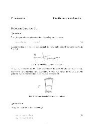
The IEA Annex 20 Two-Dimensional Benchmark Test for CFD PredictionsPeter V. Nielsen 1 , Li Rong 1 and Inés Olmedo 21 Aalborg University, Denmark2 Córdoba University, SpainCorresponding email: pvn@civil.aau.dkSUMMARYThis paper describes a benchmark test which can be used for tests of CFD predictions ofroom air distribution. The benchmark describes a box-like room with a supply slot along theside wall. Laser-Doppler measurements and hot-wire measurements are given for comparisonwith the obtained CFD predictions both for isothermal flow and for nonisothermal flow. Thebenchmark is defined on a web page, which also shows about 50 different benchmark testswith studies of e.g. grid dependence, numerical schemes, different source codes, differentturbulence models, RANS or LES, different turbulence levels in a supply opening, study oflocal emission and study of airborne chemical reactions. Therefore the web page is also acollection of information which describes the importance of the different elements of a CFDprocedure.The benchmark is originally developed for test of two-dimensional flow, but the paper alsoshows results for three-dimensional steady flow.INTRODUCTIONThe IEA Annex 20 two-dimensional test case was developed by the participants of the Annex20 work in 1990 as a benchmark [1]. Figure 1 shows the dimensions of the geometry.Figure 1. The two-dimensional benchmark test.The air distribution in the benchmark corresponds to the situation in a room with a slot inlet.The dimensions and flow conditions are the following: L/H = 3.0, h/H = 0.056 and Re = 5000,

where L, H, h, Re are length, height, slot height and Reynolds number, respectively.Velocities are measured in a model with W/H = 1.0 [2], and streaklines are photographed in amodel with W/H = 4.7, see figure 2, [3].Figure 2. Streaklines obtained by photographing metaldehyde particle flow. The particles areilluminated in the symmetry plane of the room.The velocity profiles for the inlet slot are also given in [1], and the following conditionsshould be used in most benchmark testsk o = 1.5 (0.04 · u o ) 2 , ε o = k o 1.5 /l o and l o = h/10 (1)where k o is turbulent kinetic energy in the supply opening, ε o is the dissipation, and l o is thelength scale.The benchmark test is divided into an isothermal case, 2D1, as described above, and anonisothermal case, 2D2, where the temperature distribution is measured along a horizontalplane in the room with heat released along the whole floor, figure 3 [3]. A small Archimedesnumber and a high velocity ensure an almost isothermal flow, and the temperature distributioncorresponds to a concentration distribution from an even distributed source along the floor. Anonisothermal test with high Archimedes number and restricted penetration of the plane walljet into the room is also introduced [1]. Those measurements are based on Scwenke’sexperiments [4].Figure 3. Position of measurement points for temperature distribution in the benchmark test.APPLICATION OF THE BENCHMARKThe benchmark is located together with three other benchmarks on the web page:www.cfd-benchmarks.comThe other benchmarks are about computer simulated manikins. They deal with mixingventilation and displacement ventilation, thermal comfort and personalized ventilation.

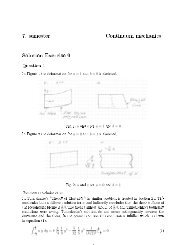
About 50 different applications of the IEA Annex 20 two-dimensional benchmark (madebetween 1974 and now) can be found on the web page. This gives the possibility to compare aprediction with other authors’ results (other turbulence models, other numerical schemes,different inlet conditions, etc.). The basic knowledge behind the benchmark test has thus beenexpanded during the years and made the benchmark test more useful. A few examples arediscussed in the following sections.Early predictionsFigure 4 shows some early two-dimensional predictions based on the vorticity-streamfunction equations, ω-ψ, and on the RANS equations, [3] and [5] as well as predictions basedon RANS equations with a one equation turbulence model, [6].Figure 4. Early predictions of the velocity profile at x/H = 2.0 with different sets of transportequations, and different turbulence models.Different numerical schemesFigure 5 shows a set of predictions based on a low Reynolds number k-ε model (the LRNmodel), [7]. The results are compared at two different vertical sections. The recirculating flowis well predicted in the simulations, although the magnitude of the counter flow is slightlyunderestimated. The maximum velocity in the occupied zone is accurate with respect to bothlocation and magnitude.

Figure 5. Velocity profiles and turbulent kinetic energy predicted by a LRN model.2It is possible to compare the measured RMS value u'with the square root of the turbulentkinetic energy k because the flow can be considered as a flow with wall jet profiles ( k ~21.1 u ' ). The figure shows that the predicted level of turbulence is in good agreement withthe measurements.Large Eddy Simulations, LES, can be used to obtain detailed information on turbulence,which can not be achieved by the traditional time-averaged turbulence models. The turbulence2is predicted in details, and it is possible to make a direct prediction of u ' . Figure 6 showssome early predictions by Davidson and Nielsen [8]. It was difficult to get sufficientintegration time for the calculation of u and2u ' .Figure 6. Time-averaged velocity and turbulence intensity in the symmetry plane predicted byLES.AB

Figure 7. Probability density function of ufloor at x/H = 1.0. See [8].The probability density function of uuouoclose to the ceiling at x/H = 2.0, and close to theclose to the ceiling at x/H = 2.0 has a well-definedmean velocity, and the velocity fluctuates around the mean velocity in a symmetricaldistribution, figure 7A, while the flow close to the floor at x/H = 1.0 is asymmetric (has askewness) with a probability of both a negative and a positive velocity, figure 7B.Different turbulence modelsTwo-dimensional steady state predictions with different turbulence models indicate somedifferences, especially in two of the corners as shown in figure 8, [9]. The grid is identical inall four cases, which means that the difference in the flow can be ascribed to the turbulencemodels used to predict the two-dimensional flow. The predictions with the SST model showespecially a large recirculating flow in the occupied zone below the supply slot 0 < x/H < 1.5.Similar results have been obtained by Voigt [10]. It is not possible to fully exclude this flowpattern from the observation of the streaklines shown by photos as in figure 2, but it does notcorresponds to the Laser-Doppler measurements in the benchmark.Figure 8. Two-dimensional isothermal and steady state simulations of the Annex 20 2Dbenchmark test. Four different turbulence models are used together with the RANS equations.THREE-DIMENSIONAL STEADY STATE PREDICTIONSThe benchmark was originally selected for the simulation of steady two-dimensional flows forthe IEA Annex 20 work back in 1990. The flow in the benchmark was considered to be twodimensionaland steady, but three-dimensional unsteady flows could, at least in principle,occur. LES predictions indicate an asymmetric probability density function at the floor at x/H= 1.0 with a probability of both negative and positive velocities, figure 7B, and measurementsin rooms with L/H ≥ 4.0 and W/H = 4.7 do also show unsteady flow at the floor for 0 < x/H

when different turbulence models are used. Figure 9 shows the flow in the symmetry plane ofthe room for the k-ε model and the SST model. The three-dimensional prediction with the k-εmodel looks similar to the two-dimensional predictions in figure 8, while the threedimensionalprediction with the SST model is slightly different from the two-dimensionalversion in figure 8. The large recirculating flow in the occupied zone below the supply slot isreduced compared to the flow in the two-dimensional case. This change in the flow towardsthe flow predicted by the other turbulence models could be a result of having threedimensionalflow, but it could not be fully excluded that the use of a different grid might havesome influence. (The two-dimensional predictions, figure 8, are made in a structured grid,while the three-dimensional predictions in figure 9 and 10 are made in an unstructured grid).k-ε modelk-ω modelSST modelFigure 9. Three-dimensional isothermal and steady state simulations of the Annex 20 2Dbenchmark test. Three different turbulence models are used together with the RANSequations.The difference between a two-dimensional k-ω prediction and a three-dimensional k-ωprediction of the flow can be explained by looking at the flow in the occupied zone. Figure 10show the three-dimensional steady flow predicted by the k-ω model. The flow in the middleplane is very different from the flow close to the side wall. A horizontal section in theoccupied zone shows how the recirculating flow in the middle plane has a higher velocitythan the flow close to the side walls. The flow in the middle of the room therefore creates twohorizontal circulations in the region below the supply opening, which ensures a fully verticalrecirculation in the middle plane. The flow is unsymmetric in the room, although the room issymmetric.The measured flow in the benchmark, [1], does not show this large difference between thevelocity distribution in the middle plane and the velocity distribution at a distance of 0.1Wfrom the side wall.Flow in middle planeFlow close to side wall (0.1W fromside wall)

Flow in horizontal plane in theoccupied zone (0.5·h above floor)Figure 10. Three-dimensional isothermal and steady state simulations of the Annex 20 2Dbenchmark test with a k-ω turbulence model solved together with the RANS equations.A study by Susin et al. [11] using three-dimensional flow concludes that the k-ε modelperformed best compared to the RNG k-ε model and the k-ω model, and that the mostsignificant differences between calculated and experimental velocity profiles were also foundalong the floor.CONCLUSIONSThe two-dimensional benchmark test, called the “IEA 2D test case” was defined in 1990 to beused in the IEA Annex 20 work.The benchmark is defined on a web page, so it can also be used in other CFD work. Therehave been a very large number of papers that use this geometry, and about 50 works arereported on the web page. This gives the possibility to compare a prediction with otherauthors’ results (other turbulence models, other numerical schemes, different inlet conditions,etc.). The basic knowledge behind the benchmark test has thus been expanded during theyears and made the benchmark test more useful.Predictions by different turbulence models show some variation in the obtained streamlinepattern. Especially the k-ω SST model gives a flow different from the flow obtained by theother models.The benchmark was originally selected for the simulation of steady two-dimensional flow,and the flow in the benchmark was considered to be two-dimensional and steady, but threedimensionalunsteady flow could, at least in principle, occur.Predictions by a steady state three-dimensional flow show streamline pattern similar to thetwo-dimensional predictions, but the SST model introduces a change in the flow which isslightly towards the flow predicted by the other turbulence models.An analysis of the three-dimensional flow predicted by the k-ω model shows a largedifference of the flow in the middle plane compared to the flow in a plane close to the sidewall. This difference could not be confirmed by the measurements in the benchmark.REFERENCES1. Nielsen, P V. 1990. Specification of a Two-Dimensional Test Case, Aalborg University, IEAAnnex 20: Air Flow Patterns within Buildings.2. Restivo, A M. 1979. Turbulent Flow in Ventilated Rooms, PhD thesis, Imperial College,London.

3. Nielsen, P V. 1974. Strømningsforhold i luftkonditionerede lokaler, PhD thesis, TechnicalUniversity of Denmark. (English translation: Flow in Air Conditioned Rooms, 1976).4. Schwenke, H. 1975. Über das Verhalten ebener horizontaler Zuluftstrahlen im begrenztenRaum, Luft- und Kältetechnik, Nr. 5, Dresden.5. Nielsen, P V, Restivo, A, and Whitelaw, J H. 1978. The Velocity Characteristic of VentilatedRooms, Journal of Fluid Engineering, Vol. 100, pp. 291-298.6. Davidson, L and Olsson, E. 1987. Calculation of Some Parabolic and Elliptic Flows Using aNew One-Equation Turbulence Model, Proc. 5 th . International Conference on NumericalMethods in Laminar and Turbulent Flow, Montreal.7. Skovgaard, M and Nielsen, P V. 1991. Simulation of Simple Test Case, Case 2D1, Internalreport for the International Energy Agency, Annex 20, Aalborg University, ISSN 0902-7513R9131.8. Davidson, L and Nielsen, P V. 1996. Large Eddy Simulation of the Flow in a Three-Dimensional Ventilated Room, Proc. of Roomvent’96, Yokohama.9. Rong, L and Nielsen, P V. 2008. Simulation with Different Turbulence Models in an Annex 20Room Benchmark Test Using Ansys CFX 11.0, DCE Technical Report No. 46, AalborgUniversity.10. Voigt, L K. 2000. Comparison of Turbulence Models for Numerical Calculation of Airflow inan Annex 20 Room, Department of Energy Engineering, Technical University of Denmark, ET-AFM 2000-01, ISBN 87-7475-225-1.11. Susin, R M, Lindner, G A, Mariani, V C, and Mendonca, K C. 2009. Evaluating the Influence ofthe Width of Inlet Slot on the Prediction of Indoor Airflow: Comparison with ExperimentalData, Building and Environment, 44, pp. 971-986.