draft manuscript - cabeceras.org

evidence for contact. They should be discarded, leaving a phonological area that is defensibleboth quantitatively and qualitatively.In a two-core analysis, there are two proposed core instead of one, resulting in a divisionof languages into four sets. The naive Bayes classifier is trained on both core along withthe control set. It then does three-way classification, and produces three scores for eachlanguage. These score indicate the similarity of each language to each of the two core andto the control set. Those that score high for either of the two cores are then evaluated forbeing plausibly connected to the languages of the core.3 Dataset and Analytical Goals3.1 SAPhonThe quantitative exploration of phonological areality presented in this paper is based on theanalysis of the phonological inventories found in the South American Phonological InventoryDatabase, version 1.1.3 (SAPhon 1.1.3; Michael, Stark, and Chang 2013). 1 In this sectionwe briefly describe the structure of the database and discuss particular decisions that wemade in populating the database and preparing it for quantitative analysis.SAPhon 1.1.3 incorporates 359 phonological inventories that have been harvested frompublished sources, or contributed by linguists currently working on the languages in question.This represents over 95% coverage of South American languages for which phonologicaldescriptions are known to exist in one form or another. The vast majority of inventories inthe SAPhon database belong to living languages, but SAPhon also includes inventories fromrecently extinct languages, such as Chamicuro (Parker 1991), as well as inventories basedon the careful interpretation and re-analysis of older resources, as in the case of Cholón(Alexander-Bakkerus 2005).To facilitate quantitative analysis, the phonological inventory of each language is codedin a comprehensive phonological feature table, in which all the segments and contrastivesupersegmental features (e.g. nasal harmony) attested in South American languages arelisted along the x-axis, and the names of all the languages in the database are listed alongthe along the y-axis. The inventory of any given language can then coded as a row of onesand zeros in the table, where the presence of a given segment for a given language is coded as‘1’ in the appropriate column, and absence coded as ‘0’. Note that this allows the exhaustivecoding of inventories, without having to decide in advance which segments or contrasts arerelevant to the exploration of areality. 2We now turn to a number of methodological and analytical issues posed by the nature ofthe data on which SAPhon is based. Since SAPhon draws data from a considerable range ofpublished and unpublished sources, issues of heterogeneity in those sources pose challengesfor development of the database, and for the analytical purposes to which we put that data.The first type of heterogeneity we must contend with is the existence of multiple, andincompatible, phonological descriptions for particular languages. Since allowing multipleinventories for a given language poses significant analytical difficulties, we generally opt for1 Available online: http://linguistics.berkeley.edu/∼saphon2 We thank Mark Donohue for sharing this very useful coding technique with us.4

selecting one inventory out of the various proposed for a given language. In doing so, we aimto select inventories given in descriptions that present the greatest amount of supportingdata and analytical detail and which have prepared by authors with the greatest amountof linguistic training. And in general we prefer inventories based on more recent work, onthe grounds that recent work takes into account both previous analyses and new data. Toimprove the quality of our judgments in evaluating conflicting analyses we also consultedspecialists in particular languages, language families, and known linguistic areas in SouthAmerica. In cases where there is compelling evidence that the differences between inventoriesproposed for a given language are due to dialectal differences, we include both dialects inthe database.The second type of heterogeneity we must contend with stems from the different waysin which linguists treat the same empirical phenomena. Different analytical or representationalchoices can lead to differences in the inventories given for different languages that donot reflect significant empirical differences between the inventories of the languages in question.To remove these spurious artifacts, we subject the coded inventories to phonologicalregularization prior to quantitive analysis (while leaving the original coding intact).To understand the motivation for phonological regularization, and for an demonstrationof how it is carried out, it is useful to consider a concrete some concrete examples. We firstdiscuss the treatment of non-high front vowels in Tupí-Guaraní (TG) languages. All TGlanguages exhibit two contrastive front vowels, given in descriptions as /i/ and either /e/or /E/ (and in one case, /I/). In the cases of some of the languages for which the symbolchosen to represent the front mid vowel phoneme is /e/, the description explictly indicatesthat this vowel is phonetically realized as [E] (e.g. Kamaiurá; Seki 2000), and in other TGlanguages the symbol chosen for the mid front vowel phoneme is /E/ (e.g. Nhandeva; Costa2003). In addition, there are several TG languages in which the symbol used to representthe non-high front vowel phoneme is /e/, but no information is provided as to its phoneticrealization. Crucially, no TG languages exhibit two contrastive front mid vowels, so that wenever encounter a contrast between /e/ and /E/.For purposes of the analysis presented in this paper, we treat all TG languages as havingthe same two front vowels phonologically: a high front vowel /i/ and a mid front vowel /e/.We implement this regularization by recoding the phonemes given as /e/ or /E/ in theselanguages as {e} (leaving the phonemes in the underlying database untouched). This resultof this normalization is to recast the inventories of TG languages as exhibiting no differencein their front vowels for the purposes of our quantitative analysis. And of course we extendour treatment of vowel systems of these types to all languages in our dataset, such thatwe treat all languages that exhibit only /i, e/ or /i, E/ in their inventory of front vowel asexhibiting /i, {e}/. Of course, in languages in which /e/ and /E/ do contrast, as in themajority of Macro-Ge languages, no regularization of these segments is carried out.The preceding motivation for regularization ultimately stems from the fact that linguistsvary in their choices of symbol to represent a given phoneme, but there are also methodologicaland typological motivations for regularization. First, given the phonetic similarityof [e] and [E] it is likely that not all field linguists systematically distinguish the two phonesin languages in which they do not contrast. Moreover, one would expect to often find noncontrastivevariation between these two phones within such languages, based on a variety ofphonetic and sociolinguistic factors. This means that using both /e/ and /E/ to represent the5

single mid front vowel present in different languages suggests a a greater degree of phoneticprecision across the phonological descriptions on which SAPhon is based than is probablywarranted.Second, it is clear that in cases like that of Kamaiurá, mentioned above, linguists choosephoneme label that represents not the precise phonetic value of it basic allophone (i.e. [E]),but the typologically expected phoneme in that area of the phonemic space (i.e. /e/), asdelimited by the phonemes with which it contrasts. As such, phoneme representations ofthis sort are not directly comparable to those which opt for a representation that is morephonetically faithful to the basic allophone of the phoneme (i.e. /E). Regularization resolvesthe discrepancy between these two principles for choosing phoneme symbols by convertingall ‘phonetically faithful’ phoneme symbols to ‘typologically unmarked’ ones.A second phenomenon that illustrates a more analytically profound motivation for regularizationcomes from the treatment of contrastive nasality in Southern American languages,as exemplified by the treatment of surface nasal vowels in Tukanoan languages. Briefly,surface nasal vowels are accounted for in two ways in these languages: as the surface realizationof underlying nasal vowels, or as vowels that have undergone nasalization due to amorpheme-level nasalization feature that spreads nasalization onto the vowels in question(see, e.g. Gomez-Imbert 1993 and Stenzel 2004). The former analysis tends to be commonin earlier works on languages of this family, and the morpheme-level nasal spreading analysisis typical of more recents works. There is no reason, however, to believe that there isany material empirical difference among the languages in question that would lead one toprefer the phonemic nasal vowel analysis for some languages and the morpheme-level nasalspreading analysis for other languages. Rather, these appear to be two different ways toanalyze materially similar distributions of nasal features. In cases like this too, then, we regularizethe phonological systems in question, in this case by adding nasal counterparts to alloral vowels to the phonological systems of languages that have been analyzed as exhibitingmorpheme-level nasal spreading or nasal harmony.We enumerate the regularization rules and discuss how they are applied to the SAPHondataset in Appendix A.1.3.2 Applying Core and Periphery to Andean languagesIn this paper we illustrate the Core and Periphery technique by using it to explore the Andeanphonological area, and two phonological sub-areas within this larger area, the SouthernAndean phonological area, and North-Central phonological area. In doing so we exemplifyhow the technique works when selecting cores of varying degrees of initial insightfulness.The choice of the Andean highlands as a candidate core is an obvious one for areal specialists.Büttner (1983: 179), for example, observed that Southern Andean languages exhibitsimilar phonological inventories, and observations by linguists like Dixon (1999) regardingthe phonological distinctiveness of the Andean and Amazonian regions are generally deemeduncontroversial (even if detailed evidence for such claims is not presented). Similarly, theAndes is generally recognized as a culture area (Steward and Faron 1959: 5-16) which has,at different points in time, been dominated by large empires or polities, including Wari,Tiwanaku, and the Inkas.In the first Core and Periphery analysis we carry out, we operationalize a Andean core6

as including all languages located in the contiguous mountainous region of western SouthAmerica above 2000 meters in elevevation, from Patagonia in the south to Ecuadorean Andesin the north. The 2000 meter limit clearly separates Amazonian groups whose territoryextends into the Andean piedmont from Andean peoples, and the northern limit of theEcuadorean Andes corresponds to the extent of the Andean culture area as defined by thenorthernmost limit of Quechuan expansion. We then operationalize the control region asbeginning at 1500 kms from the nearest Andean language, and extending to the furthestlimits of the continent. The 1500 kilometer-wide strip between the core and control languagesis thus occupied by the languages on which the NBC has not been trained, and are to beevaluated by the classifier for how closely they resemble core and control languages, on whichthe NBC has been trained.The second Core and Periphery analysis we perform is motivated by the observation thatalthough all Andean languages share features that distinguish them from non-Andean languages,the Southern Andean languages exhibit distinctive features not found in most Centralor Northern Andean languages, e.g. series of ejective consonants, while the latter group oflanguages exhibits distinctive features in the former group, e.g. retroflex affricates.Thesefacts suggest that that it may be useful to treat the Andean area as constituted of two subcores:a Southern core and a North-Central core. There are also sociohistorical facts thatsuggest that it may be useful to distinguish two cores in this way, namely, the fact that theSouthern core corresponds roughly to extensions of the Tiwanaku empire, which extendedover a region corresponding roughly to modern highland Bolivia, and that the North-Centralcore corresponds roughly to the extension of the Wari horizon (Isbell 2008). For the purposesof this analysis, we define the Southern Andean core as all Andean languages south of theline that separates languages with ejectives from those without ejectives, with the remainingAndean languages constituting the North-Central core.4 Exploring language contact with a naive Bayes classifier4.1 OverviewA naive Bayes classifier is a probabilistic model that is used to classify objects into K classes.Such a classifier is first trained on many examples, each labeled by a human expert with theclass to which it belongs. Thereafter, when presented with a novel object, the classifier willreport with what probability the object belongs to each of the K classes.A common application of this technology is spam filtering. An e-mail account mayreceive dozens of unwanted messages every day, but a typical classifier is smart enough toput almost all of them into a spam folder, saving the user the trouble of ever having to lookat them. In this application there are two classes: spam and non-spam. The classifier istrained on messages that it knows to be spam (such as those the user manually flags) andthose it knows to be non-spam (such as those that the user doesn’t flag after reading). Thiscontinuously-trained classifier is applied to incoming messages, and usually works very well.A naive Bayes classifier analyzes each object by its features. In the case of e-mail, thefeatures are the words that a message contains. When an incoming message is analyzed, each7

word will push the classification toward spam or non-spam, depending on how strongly theword is associated with spam or non-spam in the messages that the classifier has been trainedon. A word such as Viagra is a strong indicator of spam, whereas most low-frequency words(such as analysis or linguistics) are weak indicators of non-spam. The classifier combines theevidence from each word to reach a verdict about the message as a whole.Adapting this technology to classifying languages is straightforward: we train a classifieron training languages from two or more classes of interest, and use it to probabilisticallyclassify test languages. The analyst provides a featural specification for each language, and aclass label for each training language. In this paper the featural specification is an encoding ofthe phonological inventory in which each feature is a phoneme that is either present or absentin the language. 3 During training, the classifier will calculate how strongly each phonemeis associated with each class. Then, in order to classify a test language, the classifier willcombine the evidence from each feature and assign K probabilities to the test language —these are the probabilities that the test language belongs to each of the K clusters.4.2 Two-way classificationA two-way classifier is a special case of a general K-way classier that can be explained insimpler terms, so it will be discussed first. Training a classifier with two classes entailscalculating a feature weight for each feature, which expresses how strongly each feature isassociated with each class. The weight for feature l is(N1lu l = log ÷ N )1[provisional].N 2l N 2N 1l is the number of training languages in class 1 that have feature l, and N 1 is the totalnumber of training languages in class 1. N 2l and N 2 are analogous quantities for class 2.The first ratio N 1l /N 2l is a comparison of the counts of feature l in the two classes. Thisis counterweighted by the second ratio N 1 /N 2 , which expresses the relative sizes of the twoclasses. The logarithm has the effect of causing the weight to be zero when the feature isneutral, positive when it is associated with class 1, and negative when associated with class2.One problem with this formula is that when any of the counts are zero, the feature weightu l ends up at either positive or negative infinity. To prevent this, we inflate the counts by asmall amount in order to regularize the result:( α + N1lu l = log ÷ α + β + N )1.α + N 2l α + β + N 2For many applications it suffices to set α = β = 1/2, but in our analyses we fit theseparameters to the data, as explained in §A.4.3 In this article, feature always refers to a feature of a language as a whole (such as the presence or absenceof a particular phoneme in the phonological inventory) rather than to phonological features such as labial orunrounded.8

Strictly speaking, the above expression gives the feature weight for the presence of afeature. It is also necessary to calculate weights for the absence of a feature, via( β + N1 − N 1lv l = log÷ α + β + N )1.β + N 2 − N 2l α + β + N 2The main difference is that counts for the presence of a feature N 1l and N 2l have beenreplaced by counts for the absence of the feature N 1 − N 1l and N 2 − N 2l . Once featureweights (for both present and absence features) have been calculated, the classifier is readyto classify.For each test language the classifier produces a scores =L∑l=1{ul if feature l is present in the test language,v l if feature l is absent in the test language.(1)This score is a summation over all features (numbered from 1 to L) of feature weights, usingu l if feature l is in the test language, or v l if feature l is not. The interpretation of the scoreis similar to that of the weights. A score of zero means that the test language is equallylikely to belong to either class; a positive score means that it is more likely to belong to class1; and a negative score means that it is more likely to belong to class 2.4.3 Probabilistic interpretationIn fact there are probablistic interpretations for the weights u l , w l and the score s. We firstapply a function S(o) = 1/(1+e −o ) to them to convert them into probabilities. This functionis plotted here.S(o) = 1/(1 + e −o )−4 −3 −2 −1 0 1 2 3 4s10This sigmoid function translates from values that have a range of [−∞, ∞], to a probability,which has a range of [0, 1]. The argument o is a log-odds, so-called because it is the log of anodds ratio. It is related to a probability p via the inverse function S −1 (p) = log p/(1 − p).S(s) is the probability that a test language belongs to class 1, conditioned on havingthe features that it has and lacking those that it lacks. S(u l ) is the probability that atest language belongs to class 1, conditioned only on the presence on feature l. S(v l ) isthe probability that a test language belongs to class 1, conditioned only on the absence onfeature l.4.4 Underlying model and K-way classificationSection 4.2 discussed naive Bayes classification from a procedural perspective. Now weengage in a brief discussion of the model that underpins the procedures. The model posits9

that our data, which comprise the training languages, the test language, and the labels forthe training languages, were generated via a set of random events, which are as follows. 4• Randomly pick a feature frequency θ kl for each feature l and each class k. This isthe probability that a language in class k will have feature l. Feature frequencies areunobserved.• Assign each language, including the test language, to one of K classes with probability1/K. 5 The assignments of the training languages are observed. The assignment of thetest language is unobserved.• For each language, endow it with feature l with probability θ kl , where k is the class ofthe language. Each feature is generated independently of the others, conditional on k.The features that a language has are all observed.With this as the premise, the classifier seeks to infer the class of the test language. Itcalculates, for each class k, the probability f(k) that the test language would be generatedby the feature frequencies of class k. From this it infers that the test language belongs toclass k with probabilityp k =f(k)f(1) + f(2) + · · · + f(K) . (2)If the feature frequencies were known, the formula for f(k) would be straightforward:f(k) =L∏ {l=1θ kl if feature l is in the test language,1 − θ kl if feature l is not in the test language.[provisional]The classifier is essentially calculating the likelihood of each choice f(k) by taking the productof the probability of generating each feature value (present or absent) in the test language.We do not know what these feature frequences are, but we can obtain some insight (albeitnot exactly the right answer) by estimating the feature frequencies directly from the data viathe formula θ kl = N kl /N k , where N kl is the number of times feature l exists among traininglanguages of class k, and N k is the total number of training languages of class k. We get:f(k) =L∏l=1{NklN kN k −N klN kif feature l is in the test language,if feature l is not in the test language.[provisional]The correct equation, which is not much more complicated, involves integrating over all possiblevalues for all feature frequencies. (See §A.3 for details.) If we posit a beta distribution4 When thinking about such models, W. C. finds it helpful to imagine a diety generating the data accordingto the procedure given, with some of the diety’s choices hidden from view. What is not hidden comprisesthe data. On the basis of this data, we infer some of the hidden things.5 In a more sophisticated variant of this model, each language is assigned to class k with some probabilityπ k . The random variable π k is not observed, and must be inferred from the data. In two-way classification,this adds a term such as log[N 1 /N 2 ] to the score of the test language. When the number of training languagesis fixed (as in our analyses) this term moves all scores up or down by a fixed amount, and does not alter anyconclusions.10

prior for each feature frequency θ kllikelihood:∼ Beta(α, β) we get the following expression for thef(k) =L∏l=1{ α+Nklα+β+N kβ+N k −N klα+β+N kif feature l is in the test language,if feature l is not in the test language.(3)This, along with Eq. 2, yields the probabilities p 1 , . . . , p K for K-way classification. Convertingthese probabilities to log-odds via s k = log p k /(1 − p k ) yields a set of K scores. WhenK = 2, the score s 1 is what was derived in §4.2 and s 2 = −s 1 . 64.5 Feature non-independence and the interpretation of resultsThe naive Bayes classifier’s name is due to the naive assumption that the features in alanguage are generated independently, given the class of the language. In reality, however, theexistence of one phoneme can be strongly correlated with the existence of another phoneme.For example, a language with /e/ often tends to have /o/, and vice-versa. Or, a languagewith one ejective stop tends to have more ejective stops. There is a sense in which having midvowelsor having ejective stops is a single “fact” about a language, but a naive Bayes classifierwill treat each fact of this sort as multiple facts. (The presence of mid-vowels is treated astwo facts: the presence of /e/ and the presence of /o/. The presence of ejective stops istreated as multiple facts about the presence of each individual ejective stop.) This kind ofmultiple counting results in inflated scores, producing an effect of exaggerated certainly.All languages show this effect to some extent, because there are many clumps of featuresthat go together, such as mid-vowels, nasal vowels, long vowels, voiced stops, aspiratedstops, ejective stops, etc. The presence or absence of any of these clumps will cause theclassification to swing about in an exaggerated way. In our analyses, we sidestep the problemby disregarding the literal interpretation of the classification probabilities and reinterpretingthem as indicators of linguistic admixture.The definition of the underlying model for a naive Bayes classifier in §4.4 makes nomention of the possibility of admixture. It is presupposed that each language derives from asingle source that is identified with the class of the language. The model allows that there israndomness in how features are generated, so there is always going to be some uncertainty inthe classification of a language, but underlyingly the features all came from the same source.In reality, however, languages are often mixed, deriving some of their features from onesource and some from another. We will use the classifier probabilities as an indicator ofadmixture. Unfortunately the coarseness of this method does not allow us to infer the6 With K-way classification, there isn’t a distinct training stage, since we do not compute feature weightsbefore scoring each language, as we do in two-way classification. When K = 2, however, the probability thatthe test language belongs to class 1 has the form p 1 = f(1)/[f(1) + f(2)]. Converting this probability to alog-odds via s = log p 1 /(1 − p 1 ) yields a score s = log f(1)/f(2), which expands tos ={L∑logl=1α+N 1lα+N 2l÷ 1+α+β+N11+α+β+N 2β+N 1−N 1lβ+N 2−N 2l÷ 1+α+β+N11+α+β+N 2if feature l is in the test language,if feature l is not in the test language.We see here that each feature value (present or absent) contributes in an additive way to the score. Comparingthis to Eq. 1 shows how the feature weights were derived.11

absolute proportions of admixture in a language. If the model reports that a languagebelongs to class k with probability 0.7, we cannot interpret that to mean that 70% of thephonemes of the language are from a source that is identified with class k. We can onlyconclude that if p k is higher for one language than for another, then the former must derivemore of its phonemes from that source than the latter.4.6 Details in applying the model4.6.1 Feature cullingFor our relativistic interpretational strategy to work, there cannot be languages that haveclassification probabilities that are significantly more exaggerated than what other languageshave. Rare features are a nuisance because they will cause this to happen. For example, thereare 112 features in our dataset that occur in exactly one language, but twelve of them occur inthe same language, Paez, despite there being 349 features in all after feature regularization.These twelve features are completely correlated, which causes the classification of Paez to begreatly exaggerated. To prevent outcomes of this sort, we have discarded all features thatoccur five or fewer times in the training languages from our analyses. In the analyses of thispaper this has amounted to discarding 280 of the 349 features in the dataset, leaving 79.Near-universal features are as unhelpful as rare features, since, when absences are rare,they can in theory clump together like rare features. We have discarded those that arepresent in all but five or fewer training languages. This has amounted to discarding /t/,/k/, /i/, and /a/ from our analyses, leaving 75 features.4.6.2 Measuring admixture in a training languageWhen using a naive Bayes classifier to discover admixture, we should not exempt the traininglanguages from scrutiny. However, it would prejudice the model for a test language to alsobe a training language. When we wish to apply the classifier to a training language in classk, we remove it from the set of training languages first. This lowers the counts N k in Eq. 3by one, and lowers the counts N kl by one for each feature l in the test language. After thisadjustment, classification proceeds as before.4.6.3 Feature deltasIn a two-way classifier, the feature weights u l and v l give measures of the association betweenclass 1 and, respectively, the presence or the absence of feature l. Having two weights foreach feature is cumbersome if all we wish to know is the degree of association between afeature and a class. Using the formulas in §4.2 we define a measure called delta:δ l = u l − v l = log( )α + N1l− logβ + N 1 − N 1l( )α + N2l.β + N 2 − N 2lThis measure is zero if the feature is neutral, positive if it is associated with class 1, andnegative if it is associated with class 2. We can generalize delta to K-way classification by12

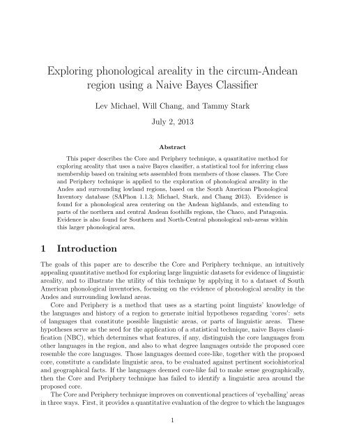
6420-2-4-6pʰpʼ tʼpbdqʰqʼʈ ʂ tʃ ʼtʃʰ q ɲtʃskʼ kʰtʰ tsm n ʂ ʃɡ z ɬ w jdʒ kʷ ŋ ɸɣ eːhʎχxlɾ iː aːoː̃̃ʔ ŋʷ β f iː̃ ẽː ɛ̃ãːɔ̃ õːe ɛ ɔ oi ẽ ã õ ũ ɨuũːuːɨːɨː̃əə̃əː ə̃ː ɤ toneɨFigure 1: Deltas for single core Andean analysisdefining a set of K deltas for each feature:δ kl = log(hkl)− log1 − h kl( ∑j≠k h )jl∑j≠k 1 − h ,jlwhere h kl = (α + N kl )/(α + β + N k ). The summations are from 1 to K, excluding k. Theelement δ kl is zero if feature l is neutral with respect to class k, positive if feature l ispositively associated with class k, and negative if it is negatively associated with class k. Afeature that is neutral with respect to all K classes will have zeros for all K deltas.5 Results and Discussion5.1 Single Andean CoreThe feature deltas (henceforth ‘deltas’) resulting from the NBC analysis of the Andean coreare given in Figure 1. Positive deltas contribute to the classification of the languages thatbear them as Andean, while negative deltas contribute to the classification of the languagesthat bear them as non-Andean. The presence of phonemes like /q/ and /L/ in the inventoryof a given language thus strongly contribute its classification as Andean, while the presenceof /1/ or /ã/ strongly contribute to its classification as non-Andean.The deltas given in Figure 1 yield the distinctive phonological profile for the Andeancore given in Tables 1-4. In these tables we (somewhat arbitrarily) select a delta of ±213

p h p’ t h t’ k h k’ q q h q’tS tS h tS’ úùs S x Xñl RńTable 1: Distinctive consonants of the Andean core languages (positive deltas)B fd k w PdZhN wTable 2: Distinctive consonants of the Andean core languages (negative deltas)(p = 0.88) or as the cutoff for segments whose presence or absence is strongly characteristicof the Andean core, and deltas between 1 and 2 (0.73 < p < 0.88) and −1 and −2 as therange for segments whose presence or absence, respectively, are moderately characteristicof the Andean core. Strongly characteristic segments are given in bold, while moderatelycharacteristic ones are given in normal type face.The distinctive phonological profile of the Andean core languages is large, in the sense thata large number of segments distinguish the Andean core languages from control languages,both in terms of their presence and their absence. The size of this distinctive phonologicalprofile strongly supports that the chosen core forms part of a phonological area.The distinctive Andean consonantal profile can be positively characterized in generalterms as exhibiting contrastive aspirated and ejective stops (a contrast found also in thepost-alveolar affricate), as well as a relatively large number of affricates, fricatives, and liquids.Less common places of articulation that are positively significant to the profile includethe palatal (nasal and liquid) and uvular (stop and fricative) places of articulation. Theconsonantal profile can be negatively characterized as excluding the voiced alveolar stopand affricate, the labialized voiceless stop and nasal, voiced bilabial and voiceless labiodentalfricatives, and the glottal stop and fricative. The distinctive Andean vocalic profile ispositively characterized by vowel length only, but negatively by the absence of mid and ceni:u u:a:Table 3: Distinctive vowels of the Andean core languages (positive deltas)14

ĩ ĩ: 1 1: ˜1 ˜1: ũ ũ: tonee ẽ ẽ: E Ẽ @ @: ˜@ ˜@: o õ õ: O Õ 7ãTable 4: Distinctive vowels of the Andean core languages (negative deltas)tral vowels in their oral and nasal realizations, and for several of these vowels, their longcounterparts as well.The deltas given in Figure 1, yield the NBC scores given in Appendix A.5.1, which areplotted with their locations in Figure 2. Languages with NBC scores near zero, and hence,difficult to classify as either Andean or non-Andean, appear in white. The higher a language’sNBC score, the greater its red saturation, while the lower (i.e. large negative) a language’sNBC score, the greater its blue saturation.Inspection of Figure 2 reveals that a penumbra of languages with large NBC scoressurrounds the posited Andean core, which is, unsurprisingly, dense with languages withvery high NBC scores. Following our discussion of the interpretation of NBC scores in§4.5, the high NBC scores of many of the languages in the circum-Andean peripheral regionindicate that their phonological inventories much more closely resemble those of core Andeanlanguages than those of the control languages, suggesting admixture with Andean languages.Inspection of Figure 2 also reveals that there is a gradual tapering off with distance fromthe Andean core of how Andean-like languages in the circum-Andean region are. The peripheryof this phonological area is thus diffuse, lacking a clear boundary separating peripherallanguages that are unambiguously members of the phonological area, such as Yanesha’ [ame],from those that are clearly not, such as Aguaruna [agr]. If we consider any language with anNBC score greater than zero to be a candidate for membership in the area, and (somewhatarbitrarily) any language with an NBC score in the 95th percentile or greater to be a strongcandidate for membership in the area, we obtain a partitioning of the periphery into ‘strong’and ‘weak’ members of the linguistic area. These peripheral members of the Andean coremostly cluster geographically, as indicated below, and displayed in the more detailed mapsin Figures 3-5.ecuadorean foothillsStrong: Cha’palaa [cbi] (Barbacoan)Weak: Kamsá [kbh] (isolate)huallaga valleyStrong: Chamicuro [ccc] (Arawak), Cholón [cht] (isolate)Weak: Shiwilu [jeb] (Cahuapanan), Candoshi [cbu] (isolate)southern peruvian foothills15

Andean coreControl classTest language onlyFigure 2: Languages of South America (two-way Andean core NBC scores)16

chacoStrong: Yanesha’ [ame] (Arawak)Weak: Ashéninka (Apurucayali [cpc] and Pichis [cpu] dialects) (Arawak)Strong: Vilela [vil] (isolate), Maká [mca], Chulupí [cag] (both Matacoan)Weak: Wichí [mtp] (Matacoan), Toba Takshek [tob tks], Toba Lañagashik [tob lng],Mocoví [moc] (both Guaicuruan)patagoniaStrong: Ona [ona], Haush [ona mtr], Günün Yajich [gny], Tehuelche teh (all Chon)Weak: Alacalufan (Northern [alc nth], Central [alc cnt], and Southern [alc sth]dialects) (Alacalufan)miscellaneousWeak: Arabela (Zaparoan), Leko [lec] (isolate)lowland quechuan languagesStrong: Ferreñafe Quechua [quf], Inga (Jungle dialect) [inj], Napo Quichua [qvo],San Martín Quechua [qvs], Santiago del Estero Quechua [qus]In several of these regions, such as the Ecuadorean foothills, the Huallaga River valleyregion, and the Southern Peruvian Foothills regions, significant contact between speakersof Andean languages and the relevant non-Andean languages is either known to have takenplace, or such contact is generally plausible, due to geographical proximity and the ubiquityof trade between adjacent highland and lowland regions.Somewhat more surprising is the fact that Patagonia and the Chaco constitute an essentiallycontiguous phonological area with the southern Andes. Although there is evidenceof trade between the Tiwanaku polity and the inhabitants of the Chaco between approximately100 AD and 1100 AD (Angelo and Capriles 2000, Lecoq 2001, Torres 2006), it isunclear whether those relations would have been sufficiently intense to produce the kindof convergence we see between the southern Andean languages. Nevertheless, one Chacoanlinguistic isolate (Vilela) and Chacoan languages of the Matacoan and Guaicuruan familiesexhibit features strongly statistically associated with the Andean highlands, including ejectives,uvular consonants, and the palatal lateral. There is even less evidence of significantcontact between Patagonian peoples and southern Andean ones, but the former languageslikewise exhibit features characteristic of the Andean core languages. It should be notedthat in Pre-Colombian times, the territory occupied by speakers of Patagonian languageswas contiguous with that occupied by Chacoan peoples (Viegas 2005: 30), raising the possibilitythat the similarity between Andean and Patagonian languages arose not from directcontact between the languages of these two regions, but was mediated by Chacoan languages.Significantly, whereas the patterning of circum-Andean languages with languages of theAndean core further to the north are explicable as instances of relatively local and recent17

cbiqviinbkbhinjseyquwqxlzroqvoarlhuujivanbcbujebcccmyrcodmcfqufqukqvspnoqvcchtqwaqxnqubcpushpcpcsyaameqvn_cajqvn_tarqxwFigure 3: Languages of North Andes and Circum-Andean regions (two-way NBC scores)jqr18

inpjqrquyquzayr_muyqulureleccawbrgcaxayr capayr_chlnhdkuzmtpcrqcaglulqustob_tksvilaxb mocmcaFigure 4: Languages of Central Andes and Circum-Andean regions (two-way NBC scores)19

arngnyalc_nthtehteh_tshalc_cntalc_sthonayagona_mtrFigure 5: Languages of Patagonia (two-way NBC scores)20

convergence of peripheral languages to Andean core languages, the phonological arealityfound in the Chacoan, Patagonian, and southern Andean languages partake does not exhibitclear directionality, and the precise circumstances that led to phonological convergence inthe area are less clear, suggesting that much older, and possibly multilateral, processes ofphonological borrowing are responsible for the large scale phonological areality we see in theSouth American Cone.In addition to the languages enumerated above, which comprise an essentially contiguousregion with the Andean highlands, we find three other languages with positive NBC scoreswhose participation in the Andean and circum-Andean phonological area is dubious. Theselanguages, listed below as outliers, obtain their high NBC scores due, in large part, tohaving aspirated stops and/or a palatal lateral in their phonological inventories. Given theprobabilistic nature of NBC results, and the great distance of these languages from theAndean core, which renders historical contact with the Andean core languages extremelyunlikely, we conclude that these languages simply bear a chance resemblance to the languagesof the Andean core.outliers:Strong: Yawalapití [yaw] (Arawak)Weak: Yucuna [ycn] (Arawak), Yaathe [fun] (Macro-Ge)5.2 Southern and North-Central CoresAlthough there are sound reasons for positing a single Andean core, there are also linguisticand socio-historical reasons to suspect that the Andean highlands exhibit linguisticallydistinguishablesub-areas. For example, simple inspection of Andean phonological inventoriesreveals that southern Andean languages exhibit a three way aspirated/ejective/plain stopcontrast and uvular consonants, whereas these features are rare or entirely absent in centralor northern Andean languages. The social histories of the two regions are also quite different,with the southern Andes historically dominated first by the Tiwanaku polity and then byAymaran peoples, who only partially penetrated into the central Andes (Adelaar 2012: 578).The central and northern Andes, in contrast, were dominated first by the Wari horizon andlater by Quechuan peoples, who penetrated into the southern Andean region only shortlybefore the arrival of Europeans.Motivated by these observations, in this section we present the results of a dual core analysisthat distinguishes a Southern core and a North-Central core, where the former consistsof all Andean languages south of a line that groups Jaqaru and Cuzco-Collao Quechua withthe Southern core, and Ayacucho Quechua with the North-Central core. 7 The deltas for theSouthern core are given in Figure 6, and the associated distinctive phonological profile isgiven in Tables 5-8, while the deltas for the North-Central core are given in Figure 7, andthe associated distinctive phonological profile is given in Tables 9-12.As evident from the deltas and distinctive profiles presented above, the two cores exhibitsignificant phonological differences, while sharing some features that distinguish them both7 This line was chosen to group together the Andean languages with a three-way contrast between plain,aspirated, and ejective stops.21

qʼ qʰ6 pʼ tʼ tʃ ʼ kʼtʃʰ4pʰ qkʰtʰχ2x ʎɲ s ɬtʃ kʷɣ lʂ jiːeːaː oːɾ0 p ts m nbŋʈ ʂ ʔʃ he owŋʷ β f iː̃ ẽː ɛ̃ ãː ɔ̃-2dʒɸ zɛ ɔ-4 d ɡi ̃ ẽ ã õ ũ ɨ ̃ɨuːuõː ũːɨːɨː̃əə̃əː ə̃ː ɤ tone-6Figure 6: Southern Andean core deltasp h p’ t h t’ k h k’ q q h q’tS h tS’s x Xl ìńñTable 5: Distinctive consonants of the Southern Andean core languages (positive deltas)d g PdZ úùF B f z SwTable 6: Distinctive consonants of the Southern Andean core languages (negative deltas)N wi: u:e: o:a:Table 7: Distinctive vowels of the Southern Andean core languages (positive deltas)22

ĩ ĩ: 1 1: ˜1 ˜1: ũ ũ: tonee: ẽ ẽ: E Ẽ @ @: ˜@ ˜@: õ õ: O Õ 7ã ã:Table 8: Distinctive vowels of the Southern Andean core languages (negative deltas)6420-2-4-6ʈ ʂ ɲ ʃ ltʃɡ s zts ʎwp b d mdʒ n ɸɾʂ xuiː aː uːq ŋ χj hpʰ tʰ kʰ ŋʷ β f iː̃ ẽː ɛ̃ ãː ɔ̃ õː ũː ɨː̃ɬ ɣ ɛ ɔ ɨːəkʷtʃʰpʼ tʼ tʃ ʼ qʰ ʔ i ̃ ẽ eː ã õ oː ũ ɨ ̃kʼ qʼɨe oə̃əː ə̃ː ɤ toneFigure 7: North-Central Andean core deltasts tS úùs z SglńñTable 9:deltas)Distinctive consonants of the North-Central Andean core languages (positive23

p h p’ t h t’ k h k’ k w q q h q’ PtS h tS’B fGìTable 10: Distinctive consonants of the North-Central Andean core languages (negativedeltas)i: u:a:Table 11: Distinctive vowels of the North-Central Andean core languages (positive deltas)N wfrom languages outside these cores. Consonantal features that positively characterize thedistinctive phonological profiles of both Andean cores include /s l ń ï/, and those thatnegatively characterize both cores include /∼B ∼f ∼N w ∼P/. Vocalic features that positivelycharacterize both cores include /i: u: a:/, while those that negatively characterize theminclude the absence of central vowels and nasal vowels. Both cores also lack tone.Other features have large positive deltas for one core, but negative ones for the other.These are features that not only distinguish the cores from control languages, but from eachother. Thus, for examples, ejective and aspirated consonants have positive deltas for theSouthern Andean core, as do uvular stops and the lateral fricative /ì/, but negative deltasfor the North-Central Andean core, whereas the converse holds for /tù g z S/.Yet other features exhibit a significant positive or negative delta for one of the cores, butdoes not emerge as significant (either positively or negatively) for the other core. For theSouthern core these include /x X/ and the absence of /d F w 7 /. In contrast /ts/ is positivelyassociated with the North-Central core profile and /G/ negatively with it, but neither aresignificant for the Southern core. Turning to the vowels, both cores are negatively associatedwith central vowels, but the North-Central core exhibits a stronger negative association withshort mid-vowels, as /e o/ are not significantly negatively associated with the languages ofthe Southern core.ĩ ĩ: 1 1: ˜1 ˜1: ũ ũ:e e: ẽ ẽ: E Ẽ @ @: ˜@ ˜@: o o: õ õ: O Õ 7ã ã:Table 12: Distinctive vowels of the North-Central Andean core languages (negative deltas)24

On the basis of the deltas given in Figs 6&7 we calculate the three-way NBC scores, whichare plotted in Figure 8. The results of three-way analysis differ from the two-way single coreresults in that instead of simply providing a single-dimensional measure of how core-like orcontrol-like a given language is, the dual core results indicate to what degree a given languageresembles the languages of either of the two cores, as well as the non-core languages. In termsof the admixture interpretation of the NBC results, then, the dual core NBC results indicatethe degree of admixture of three groups: the Southern Andean core, the North-Central core,and non-core languages. In point of fact there are no instances of significant Southern/North-Central admixture, and the significant admixtures are all between either the Southern andNorth-Central cores and the non-core languages.The qualitatively most striking and significant result of the dual core analysis is thatthe majority of the languages of the Andean periphery identified in the single core analysisdo in fact align with one of the cores, and do so in a geographically plausible manner.Thus, languages which exhibit high Southern Core NBC scores are in general more closelylocated to the Southern Core than the North-Central Core, and conversely for languages withhigh North-Central NBC scores. The fact that the Andean-like languages in the peripheralregion pattern with the nearest core, rather than being randomly associated with either subcore,indicate that convergence between circum-Andean languages and Andean languages isgenerally a relatively local effect associated with each sub-core.The principal way in which the results of the dual core analysis of the languages in thecircum-North-Central Andean area differ from the results of the single core analysis is toinclude more geographically proximal languages of this peripheral region in the phonologicalarea, or to increase how strongly they pattern with the languages of core, as listed belowand displayed in Figure 9. Kamsá [kbh], Shiwilu [jeb], Candoshi [cbu], for example, havegone from being weak members of the area to being strong members, and Panobo [pno] hasgoing from not being even a weak member of the area to being a strong member. Likewise,Andoa [anb], Sápara [zro], and Muniche [myr] went from being non-members to being weakmembers. All the new members of the area formerly had small negative NBC scores, andthe change in the deltas against which they are being evaluated has pulled them into therange of positive NBC scores.Languages of the North-Central Andean PeripheryEcuadorean foothillsStrong: Kamsá [kbh], Cha’palaa [cbi]Weak: Andoa [anb], Sápara [zro]Huallaga ValeyStrong: Shiwilu [jeb], Cholón [cht], Candoshi [cbu]Weak: Muniche [myr]Southern Peruvian foothillsStrong: Yanesha’ [ame], Panobo [pno]25

Northern-Central Andean coreSouthern Andean coreControl classTest language onlyFigure 8: Languages of South America (three-way NBC scores)26

Some languages, however, have ended up being excluded from membership in the North-Central area as a result of the dual core analysis, including Chamicuro [ccc], which wasformerly a strong member of the (single core) Andean area, and Ashéninka (Apurucayali[cpc] and Pichis [cpu] dialects) and Arabela [arl], which were formerly weak members ofthe area. In the case of the Ashninka varieties, they appear in the region of the tri-polarplot that suggests admixture of non-core features with both Southern and North-Centralfeatures, a result that is consistent with their location near the boundary of the Southernand North-Central cores. Chamicuro, in turn, just barely misses being a weak member ofthe North-Central area; although it exhibits strongly positive North-Central features like theretroflex affricate, and less strong ones, like the palatal lateral, it also exhibits mid-vowelsand glottal stop, which are strongly negatively weighted for this core.The languages in the periphery that pattern with the Southern sub-core are given below;plots of the languages of Patagonia and the Southern Andes and adjacent regions are givenin Figures 10&11.Languages of the Southern Andean PeripheryChacoStrong: Maka [mca], Vilela [vil], Wichí (Mission de la Paz dialect) [mtp]Weak (non-core admixture): Chulupí [cag]PatagoniaStrong: Alacalufan (Northern [alc nth], Central [alc cen], and Southern [alc sth]dialects), Ona [ona], Haush[ona mtr], Tehuelche [teh]As in the case of the North-Central core, several languages have gone from being weakmembers of the single Andean core to being strong members of the Southern sub-core,including Wichí [mtp] and the Alacalufan languages [alc nth, alc cen, alc sth]. Chulupí[cag] has experienced the opposite fate, and Günün Yajich [gny] has gone from being astrong member of the area to being excluded, while Leko [lec], Toba Takshek [tob tks],Toba Lañagashik [tob lng], and Mocoví [moc] have gone from being weak members to beingexcluded. All of the languages excluded under a strict interpretation of NBC scores do,however, occupy regions near the zero log-odds line, a point we return to in the discussionin §6.In addition to the instances of convergence we identify between Andean languages andlanguages in the circum-Andean foothills and lowlands, there is also evidence of convergenceof Quechuan languages to the non-Quechuan languages of the Southern core. This clearfrom the fact that Bolivian Quechua [qul quh] and Cuzco-Collao Quechua [quz] emergedwith very high Southern Andean NBC scores. Other Quechuan languages have negativeNBC scores for this core, indicating that Bolivian and Cuzco-Collao Quecha have been sosignificantly affected affected by contact with non-Quechuan Southern core languages thattheir phonological inventories pattern with those of these latter languages, rather than theQuechuan languages to which they are genetically related. Santiago del Estero Quechua ishe next more non-North-Central-like Quechuan language, presumably due to the fact that27

cbiqviinbkbhinjseyquwqxlzroqvoarlhuujivanbcbujebcccmyrcodmcfqufqukqvcqwaqvs pnochtshpsyaqxnqubcpucpcameqvn_cajqvn_tarqxwjqrFigure 9: Languages of the Northern Andes and Circum-Andean regions (three-way NBCscores)28

inpjqrquyquzayr_muyqulureleccawbrgcaxayr capayr_chlnhdkuzmtpcrqcaglulqustob_tksvilaxb mocmcaFigure 10: Languages of the Central Andes and Circum-Andean regions (three-way NBCscores)29

arngnyalc_nthtehteh_tshalc_cntalc_sthonayagona_mtrFigure 11: Languages of Patagonia (three-way NBC scores)30

its speakers migrated to the Argentinean pampas during the latest stages of the expansionof the Inka empire (Adelaar and Muysken 2004). At the same time, Jaqarú [jqr], a languagebelonging to the Aymaran language family, although still solidly patterning with Southerncore languages, more closely resembles North-Central core languages than any of the Aymaranlanguages to which it is genetically related. Since Jaqarú is far to the north of theother Aymaran languages, and adjacent to Quechan languages of the North-Central core,its greater similarity to these languages reflects a history of contact with these Quechuanlanguages.6 DiscussionHaving demonstrated how Core and Periphery operates in exploring a particular set ofhypotheses about linguistic areality, it is important to clarify a number of properties ofthis method. First, Core and Periphery is not a method which allows one to simply feedin data to an algorithm without any knowledge of the relevant languages or regions. Coreand Periphery crucially capitalizes on specialists’ linguistic and non-linguistic knowledgeboth to to generate fruitful initial hypotheses, i.e the core and control language sets, and insubsequent interpretation of the results, i.e in evaluating the plausibility of language contactbetween core and peripheral languages for languages with high NBC scores. What Core andPeriphery does provide is an intuitively straightforward means to explore large datasets forevidence of areality, by providing identifying features that distinctively characterize givengroups of languages, and a quantitatively explicit measure of similarity between groups ofspecified languages.Another important characteristic of Core and Periphery is that it bases its evaluation oflanguages as being similar to core or control languages on the basis of the totality of deltas,and is thus most effective in identifying the results of language contact that involve broadconvergence in the phonological inventories of the languages being examined. Instances oflanguage contact in which only a small number of segments are borrowed between languagesmay pass undetected by Core and Periphery, since the contribution of a small number ofborrowed segments for the trained NBC may be insufficient to classify a given languagewith the core in question. This lack of sensitivity of Core and Periphery can be seen asboth a strength and a weakness, of course: it makes the method quite conservative incertain respects, but it potentially fails to identify instances of borrowing by virtue of thisconservatism. And with respect to the issue of convergence, it is important to note thatdespite the methodological priority of the cores (i.e. that they are selected first), no claimsabout directionality of borrowing between core and periphery languages obtain from theCore and Periphery method. There is no reason that, in principle, peripheral languagescannot be the original historical source of the segments that characterize a given phonologicalarea. In these respects, then, Core and Periphery is a somewhat blunt tool: it is useful foridentifying areality characterized by broad similarity among phonological inventories, butdoes not indicate the sources of the segments borrowed in the development of the phonologicalarea.Another crucial characteristic of Core and Periphery is that the NBC scores it generatesare gradient, rather than categorial. On the one hand, this characteristic is a strength of the31

technique, since this feature makes the technique well-suited to analyzing areas with diffuseperipheries (see below), as it allows any degree of similarity to or admixture with the coreor control languages. On the other hand, the gradient nature of NBC scores introduces asdegree of arbitrariness if we seek to choose an NBC score to serve as a cutoff for identifying alanguages as being, say, either core-like or control-like for the purposes of evaluating areality.To see the somewhat arbitrary nature of the cutoff, consider the NBC score=0 cutoff that wechose in this paper to distinguish core-like from control-like languages. This cutoff is actuallysomewhat conservative, as can be appreciated by considering languages that exhibit smallnegative NBC scores.These turn out to be predominantly located close to the edge of theAndean core (as defined by the 2000m contour line), an unexpected result if all languageswith negative NBC scores were indeed wholly unaffected by contact with the relevant corelanguages. The significant clustering of circum-Andean languages in the region of smallnegative NBC scores would be explained, however, if these language were sufficiently affectedby contact with Andean languages to raise their NBC scores from their ‘pre-contact’ scores,but not quite enough to give them positive NBC scores. 8 In short, the effect of contactwith core Andean languages raises the NBC scores of the non-core languages in the circum-Andean periphery, but in some cases, not sufficiently for them to pass the zero NBC cutoff.The zero NBC cutoff is thus a relatively stringent criterion, in that it effectively excludeslanguages from the Andean core that were plausibly affected by contact with languages ofthe Andean core. In any event, it is clear that although the vicinity of zero is a significantregion in distinguishing core-like from control-like languages, it is not possible to choose asingle cut-off value without introducing a degree of arbitrariness.The issue of difuseness of the periphery just raised suggests that it would be useful toconsider the strengths and weaknesses of the Core and Periphery technique in terms of theareas it is well suited to study. An a priori evaluation of the possible results of borrowingbetween languages allows to identify three parameters along which linguistic areas may differ:distinctiveness, core-homogeneity, and diffuseness. An area exhibits distinctiveness if itexhibits linguistic features that are otherwise not widespread in the larger region of whichit forms a part (where a feature may also include the absence of a linguistic element orstructure). Note that distinctiveness is sometimes invoked as definitional of a linguisticarea, and while distinctiveness does make areas conspicuous, it is clear that pairwise ormultilateral borrowing of features may also result in an area coincidentally merging intoa larger background. 9 An area exhibits core-homogeneity if it is possible to identify a8 It would be useful for purposes of identifying the effects of contact in instances like this to have a measureof the degree to which a language diverges from related languages in the direction of neighboring languagesto which it is not genetically related. The Relaxed Admixture Model, discussed in Chang and Michael (thisissue), essentially provides a measure of this sort.9 Consider the following scenario: An isolated mountain valley contains four languages (A, B, C, D) fromdifferent linguistic families that have converged linguistically due to long term linguistic exogamy. At somepoint, speakers from another language (E), belonging to a larger language family that surrounds the valley,migrates into the valley and is eventually incorporated into the linguistic exogamy system. After severalcenturies, languages A, B, C, and D converge linguistically to E due to the significant prestige that (E), forthe sake of argument, possesses. As a result, the languages of the isolated mountain valley are now no longerdistinctive with respect to the surrounding languages, which belong to the same family as E. Nevertheless,because of the intense sharing of linguistic features in the mountain valley, we wish to treat it as a linguisticarea.32

elatively contiguous set of languages within the area that are all very similar in the linguisticfeatures being examined, either due to common descent or to long-term multilateral contactthat has led to convergence to a shared linguistic profile. An area exhibits diffuseness ifthe area has a fuzzy boundary, i.e. a sizeble zone surrounding the core area over which theconcentration of core features gradually taper off.In light of these parameters, we can first observe that since the NBC scores that theCore and Periphery technique generates are continuous, it is well suited for the study oflinguistic areas with diffuse boundaries. It should be noted that non-diffuse boundaries poseno problems for the method, and such areas can in fact resolve the issue of arbitrariness ofthe cutoff point by yielding natural breaks in the NBC scores associated with a propitiouslychosencore.Next, it is clear that Core and Periphery will only serve to identify distinctive areas, sincein order NBC to be able to sort the languages of the periphery into core-like and control-likelanguages, it is necessary that core and control languages be sufficiently different to yieldsignificantly different feature weights.Finally, Core and Periphery is significantly affected by the degree of homogeneity of aposited core. An important lesson to be gleaned by comparing the single core Andean NBCresults and the dual core Southern and North-Central NBC results, for example, is thatcombining two relatively homogeneous cores into a single less homogeneous core can reducethe efficacy of the NBC in identifying what are probably legitimate members of linguisticareas. In the Andean case examined above we can see how this occurred. By combiningthe cores in the single core analysis, for example, NBC scores were based on high deltasfor ejective and aspirated consonants, and lower magnitude negative deltas for short midvowels, the retroflex affricate, and the post-alveolar fricative, tilting the single Andean coreprofile towards the Southern Andean language. This resulted in eventual the exclusion fromthe Andean periphery of some languages in the foothills and lowland regions proximal thenorthern and central Andes because languages in this region converge not to the distinctiveprofile of the unified Andean core, but to that of the North-Central core, which in fact yieldsnegative deltas for ejective and aspirated consonants and mid vowels, and large positivedeltas for the retroflex affricate and the post-alveolar fricative.Core-heterogeneity can also pose difficulties because few or no segments may prove to exhibitlarge deltas, due to the considerable linguistic diversity of the core. However, as Michaeland Chang (this issue) show with a different technique, there do in fact exist ‘mosaic areas’in which language contact has led to borrowing among languages, without convergence to acommon phonological profile among the set of languages involved in borrowing relationships.The Core and Periphery technique is thus effective for identifying and delimiting linguisticareas that are distinctive and relatively core-homogeneous, and easily handles diffuseareas (though non-diffuseness poses no difficulties). And as we saw, the two Andeansubcores, and their corresponding proximal circum-Andean regions constitute a distinctive,core-homogenous, and diffuse phonological areas.33

7 ReferencesAdelaar, Willem. 2012. Languages of the Middle Andes in areal-typological perspective:Emphasis on Quechuan and Aymaran. In Lyle Campbell and Veronica Grondona(eds.), The Indigenous Languages of South America: A Comprehensive Guide, pp.575-624. Berlin: Walter de Gruyter.Adelaar, Willem and Pieter Muysken. 2004. Languages of the Andes. Cambridge UniversityPress.Angelo, Dante and José Mariano Capriles. 2000. La importancia de las plantas psicotrópicaspara la economia de intercambio y relaciones de interacción en el altiplano sur Andino.Complutum 11: 275-284.Büttner, Thomas. 1983. Las lenguas de los Andes centrales: Estudios sobre la clasificacióngenetica, areal y tipológica. Madrid: Ediciones Cultura Hispanica del Instituto deCooperación Iberoamericana.Dixon, R.M.W. 1999. Introduction. In R.M.W. Dixon and Alexandra Aikhenvald (eds.),The Amazonian Languages. Cambridge University Press.Gomez-Imbert. 1993. Problemas en torno a la comparación de las lenguas tucano-orientales.In María Luisa Rodriguez de Montes (ed.), Estado actual de la clasificación de laslenguas indígenas de Colombia, pp. 235-267. Bogotá : Instituto Caro y Cuervo.Isbell, William. 2008. Wari and Tiwanaku: International identities in the Central AndeanMiddle Horizon. In Helaine Silverman and William Isbell (eds.), Handbooks of SouthAmerican Archeology, pp. 731-760. Springer.Lecoq, Pierre. 1991. Sel et archeologie en Bolivie. De quelques problèmes relatifs à la occupationpr´‘hispanique de la cordillère Intersalar (Sud-Ouest bolivien). PhD dissertation:Universite de Paris 1.Michael, Lev, Will Chang, and Tammy Stark (compilers). 2013. South American PhonologicalInventory Database v.1.1.3. Available online: http://linguistics.berkeley.edu/ saphon/en/Stenzel, Kristin. 2004. A reference grammar of Wanano. University of Colorado, PhDdissertation.Steward, Julian and Louis Faron. 1959. Native peoples of South America. New York:McGraw-Hill.Torres, Constantino Manuel. 2006. Anadenanthera: Visionary plant of ancient South America.Routledge.Viegas, J. Pedro Barros. 2005. Voces en el viento: Raíces lingüísticas de la Patagonia.Buenos Aires: Mondragon Ediciones.34

AAppendixA.1 Inventory regularization rulesWe regularize phonological inventories in a procedural way, with a series of replacementrules, as given in the tables below. With consonants, we replace every sound in the firstcolumn of the following table with the sound in the second column, unless the sound in thesecond column is already in the inventory.l j → LJ → ZV → BWith vowels, the procedure is similar, but more elaborate. As with consonants, we try toreplace each sound in the first column with the sound in the second column, but we alsotry to replace any sound that contains the character in the first column by replacing thematched character with the character in the second column. (For example, the rule 0 → 1will cause us also to try 0i → 1i, 0: → 1:, ˜0 → ˜1, etc.) These replacements are not carriedout if the second character already exists as a sound, or as part of a sound, in the inventory.The vowel replacement rules are as follows.0 → 1W → 1@ → 12 → 1U → uO → o7 → oI → ie → iE → eA → aThese rules are applied in order. For example, if 0 has been replaced with 1 via the firstrule, it is then no longer possible for W to be replaced with 1 via the second rule.Finally, if the language has nasal harmony, we add the nasal version of each oral vowelto the inventory. This makes it easier to compare languages that have nasal harmony withsimilar languages where a synchronic analysis with nasal harmony has yet to be performed,or where longstanding contact has resulted in the presence of distinctively nasal vowels.A.2 Model and dataA naive Bayes classifier is underpinned by a probabilistic generative model. What follows isa formal description of the model and data, as used in our analyses. The data can be viewedas having three parts.35

• An N × L binary feature matrix X, where X nl denotes the absence (0) or presence (1)of feature l in the phonological inventory of training language n. N is the number oftraining languages and L is the number of features.• A set of labels for each training language Y = (Y 1 , . . . , Y N ), where Y n ∈ {1, . . . , K}denotes the class of language n. These labels are supplied by the analyst before analysisbegins, as are the total number of classes K.• A set of binary features for the test language X 0 = (X 01 , . . . , X 0L ), where X 0l denotesthe absence (0) or presence (1) of feature l in the phonological inventory of the testlanguage.The generative procedure that underlies the data is summarized as follows.• For each class k and each feature l, pick a feature frequency via a beta distribution:θ kl ∼ Beta(α, β).• For each language pick a label from a categorical distribution: Y = k with probabilityπ k . This is done for all training languages and the test langauge as well, but theoutcome is observed for just the training languages.• For each language n, generate each feature l via a weighted coin toss: X nl ∼ Bernoulli(θ Ynl).The subscript on θ refers to the class denoted by Y n (the class of language n) and thefeature denoted by l.In our analyses, we set π k = 1/K, but in other contexts it may make more sense to setπ k = N k /N, where N k is the number of training languages in class k. Settings for α and βwill be discussed in §A.4.A.3 InferenceThe purpose of the model is to make it possible to infer the class of the test language. Thisentails computing p k , the probability that the test language is in each class k, conditionedon the data. In standard notation, this is P(Y 0 = k | X 0 , X, Y ). By Bayes’ Theorem,P(Y 0 = k | X 0 , X, Y ) = P(X 0 | Y 0 = k, X, Y ) P(Y 0 = k | X, Y ).P(X 0 | X, Y )Writing f(k) for P(X 0 | Y 0 = k, X, Y ), this expands toP(Y 0 = k | X 0 , X, Y ) =f(k)π kf(1)π 1 + · · · + f(K)π K.Since the L features of the test language are generated independently, conditioned on theclass of the test language, we have f(k) = ∏ Ll=1 f l(k), where f l (k) = P(X 0l | Y 0 = k, X·l , Y )and X·l denotes elements of the lth column of X. Then,f l (k) = P(X 0l, X·l | Y 0 = k, Y ).P(X·l | Y )36

Note that X ml and X nl are fully independent if language m and language n belong to differentclasses. Thus the denominator factorizes intoK∏P(X·l | Y ) = P(X Ij l | Y ),j=1where I j denotes the set of test languages belonging to class j, and X Ij l denotes the entriesindexed by I j in the lth column of X. The numerator is identical, except in the factorcorresponding to class k. After casting out factors that are identical in the top and bottom,we are left withf l (k) = P(X 0l, X Ik l | Y 0 = k, Y ).P(X Ik l | Y )Writing f θkl (z) for the density function of θ kl ∼ Beta(α, β), this expands to∫ 10f l (k) =P(X 0l, X Ik l | θ kl = z, Y 0 = k, Y )f θkl (z)dz∫ 1P(X 0 I k l | θ kl = z, Y )f θkl (z)dz[ ]∫ 1 ∏0 n∈{0}∪I kz X nl (1 − z)1−X nlz α (1 − z) β dz= [ ]∏n∈I kz X nl (1 − z)1−X nl z α (1 − z) β dz∫ 10∫ 10=zα+N kl+X 0l(1 − z)β+N k −N kl +1−X 0ldz∫ 1,0 zα+N kl (1 − z)β+N k −N kldzwhere N kl is the number of training languages in class k with feature l and N k is the totalnumber of training languages in class k. We state the results of these integrals in terms ofgamma functions before simplifying:f l (k) = Γ(α + N kl + X 0l )Γ(β + N k − N kl + 1 − X 0l )/Γ(α + β + N k + 1)Γ(α + N kl )Γ(β + N k − N kl )/Γ(α + β + N k ){ (α + Nkl )/(α + β + N=k ) if X 0l = 1,(β + N k − N kl )/(α + β + N k ) if X 0l = 0.A.4 Setting hyperparametersIn §4.2 we suggested setting α = β = 1/2, which corresponds to drawing feature frequenciesvia θ ∼ Beta(1/2, 1/2). It would be better to find values for α and β such that Beta(α, β)reflects how feature frequencies are actually distributed. Though feature frequencies arehidden variables, we can estimate them via ˆθ l = N l /N, where N l is the number of languagesin the entire dataset with feature l, and N is the total number of languages. From theseestimates we compute a sample mean µ = ∑ L ˆθ l=1 l /L and a sample variance σ 2 = ∑ Ll=1 (ˆθ l −µ) 2 /L. We set these equal to the mean and variance of Beta(α, β):µ = αα + β ,σ 2 =αβ(α + β) 2 (α + β + 1) ,37

and solve for α and β to obtainα = µ2 (1 − µ)− µ,σ 2µ(1 − µ)2β = − 1 + µ.σ 2In our analyses, we use this procedure to estimate α and β before culling rare features, andget α ≈ 0.071 and β ≈ 0.755.One problem with the foregoing is that there may exist many features that we do notobserve. In our dataset there is a long tail of low-frequency features, and extrapolating fromthis, it is not unreasonable to suppose that there may be a larger, or even infinite, number offeatures that we do not observe, due to the fact that their feature frequencies are extremelylow. A naive Bayes classifier, despite working well in practice, is simply unable to accountfor this possibility. For a new model that explicitly addresses this issue, please see §7 of [?].A.5 NBC scoresA.5.1NBC scores for single core analysisThis section lists each language along with its score from the single core analysis in §5.1.Languages are given by language codes, which can be looked up in §A.6. They are orderedby the score, which represents how highland-like the language is. Training languages (thosethat define the classes on which the classifier was trained) are marked with A (Andean core)or C (control class).A ayr 56.64A caw 54.43A ayr chl 49.00A ayr muy46.82A cap 46.43A jqr 44.05A qul 43.78A quz 43.01A qvn caj 26.62C teh 26.48A qwa 23.87ame 22.61A qvn tar 22.53A qxn 21.24A ure 20.55A qub 19.97A qxw 19.32A qxl 18.30inj 16.69A quk 16.25A inb 16.16A quw 15.77quf 15.71A qvc 14.06A quy 12.83qvo 12.30qvs 11.42qus 10.64C ona mtr10.31C ona 10.02ccc 9.87A qvi 9.59mca 9.51A kuz 9.39C teh tsh 9.18cht 7.30cbi 6.93vil 6.74C gny 6.21C yaw 5.79cag 5.72C alc sth 5.69C alc nth 5.47tob tks 5.11kbh 5.03C alc cnt 4.76mtp 3.61jeb 3.53lec 3.35C fun 3.20cpc 3.06cbu 2.99moc 1.97cpu 1.51arl 1.18tob lng 0.54ycn 0.26bae 0.06cpb -0.29lul -0.3138

gae -0.97plg -1.10ign -1.41cav -1.56rey -1.85trn -1.91rgr -1.94bwi cen -1.99cox -2.01pno -2.43anb -2.56zro -2.56crq -2.57gum -2.63myr -2.86dny -3.01mcb -3.35yvt -4.18aca -4.37tna -4.53omg -4.58kvn -4.73C kgp -4.90sya -5.33C arn -5.38aro -5.72cot -6.36C wap -6.80pbb -6.82ese per -6.88cui -7.02kpc -7.03knt -7.17ywn -7.17bwi rng -7.39kav -8.03shp -8.12C ter -8.15ese bol -8.20pad -8.26yrl -8.32omc -8.56cni -8.56sha ywn -8.58ktx -8.64C hix -8.78mzp -8.81cod -9.12not -9.24tit -9.28C tpy -9.70kbc -9.93mbn -10.26ito -10.38pid -10.39pbg -10.94mpq -11.49cul -11.93C wba -11.93brg -11.95pib -12.09guo -12.09C xir -12.30ura -12.45C pab -12.49kaq -12.54cbt -12.63C prr -12.66C waw -12.73C yag -12.77mcf -13.06sae -13.37prq -13.48iqu -13.51yuz -14.24boa -14.41trr -14.45C txi -14.53cbb -14.60C kzw dzu-14.79C aap -14.80mpd -15.13tuf -15.14C arw -15.36cbr -15.53pcp -16.13axb -16.13pio -16.24jaa jmm-16.51C aoc tar -16.5239srq -16.79cbv -17.12C car ven-17.19C car esr -17.19pav -17.21orw -17.51C myp -17.68xor -17.90yup mac-18.86C pbh -19.21mbp -19.29C kbb -19.34C guc -19.57nuc -19.61chb -19.68yup irp-19.72C yar -20.06jaa jrw -20.28C mbc -20.30C guu -20.43cao -20.76arh -20.98C ake -21.01bmr -21.15jru -21.20cbd -21.76hto -22.36swx -22.83C aoc are-23.14noj -23.17C wca -23.37umo -23.39mcg -23.45pev -23.45C bor -23.52C car frg -23.55C atr -24.28C mch -24.66yui -24.71des -24.93cub -25.20ore -26.22huu -26.28acu -26.68C tri -26.73

unk -27.48C asu -27.50tav -27.52tae -27.72mts -27.81jiv -27.89bsn -28.21pyn -28.59C ako -28.68C pak -28.96cbs -29.47C way -29.54psx -30.49adc -30.65mcd -30.70agr -31.13yme -31.18hub -31.90C gub -32.77ltn -33.03C tqb -33.41boa mrn-33.60kwi -34.37C xiy -35.01yaa -35.28tba -35.30slc -35.34C gvp -36.56wmd -36.69amc -36.79gta -36.90con -36.96C mmh -37.22ash -37.28gqn -38.18nab kth-38.80C wau -38.90ayo -38.91cto -40.18C plu -41.24cof -42.73oca -43.62bdc -44.02C jur -44.26C mav -45.22C guh -45.27C sru -45.48C api -45.76C kpj -46.09skf -46.43jbt -46.58cmi -47.42yuq -47.56C awt -47.63pui -47.63auc -47.90emp -47.95C kui -48.03mpu -48.63tnc -49.11ano -49.16kxo -49.68inp -49.89C tpn -49.91C kyr -49.99cax -50.20kog -51.20gvc -52.05C yae -52.05C bkq wst-52.31tpr -52.62noa -52.79C apy -52.83C xet -52.83gyr -52.90mbr -52.93irn -52.97gvo -53.33yad -53.44C avv -53.45C xsu -53.56xwa -53.68C xav -53.72C awe -53.76C zkp -53.83aqz -53.85C urb -54.03C taf -54.08coe -54.12cas cov-54.1840C opy -54.20C myu -54.21C mbl -54.33tuo -54.60gui chn-54.70C oym jri-55.42gug -55.44cbg -55.50axg -55.75cyb -55.88C kqq -56.55arr -56.60C pta -56.70C kyz -56.88tpj -57.16C pto -57.20mot -57.20tca -57.29C guq -57.35C gvj -57.36snn -57.38amr -57.50C asn -57.56C bkq est-57.59nhd -57.66C xri -57.79apu -57.85gui izo -58.25C gun -58.38ceg -58.91cbc -58.93sri -58.93tue -58.93C kay -59.34C xer -59.60jua -59.66myy -59.84ark -59.87kwa -60.01sey -60.27C kgk -60.50C ram -60.83C suy -61.45sja -61.54bao -61.74

mbj -61.78C rkb -61.88adw -61.92pah -61.92urz -61.92pir -62.13C oym amp -62.45cas msa-62.59cas tsi -62.59C yau -63.36C apn -63.54ktn -64.60jup -64.99C yrm pac-65.21C suy tap-65.29C txu -65.38C eme -66.96C shb -67.99C xra -68.02C kre -69.16C qpt -70.17wyr -70.53yab -70.90C xok -77.43C wca yma-82.81C wca yae-82.81C guu ven-82.81C xsu kol -83.10C guu par-84.53A.5.2NBC scores for dual core analysisThis section lists each language along with its scores from the dual core analysis in §ssect:snccore.Languages are given by language codes, which can be looked up in §A.6. The three scoresrepresent the resemblence that a language has to, respectively, the Northern-Central Andeancore, the Southern Andean core, and the control class. 10 The languages are ordered by thethird score. Training languages (those that define the classes on which the classifier wastrained) are marked with N (Northern-Central Andean core), S (Southern Andean core), orC (control class).S ayr -45.29 45.29-65.21S caw -41.16 41.16-60.77S ayr chl -42.32 42.32-55.98S ayr muy-42.00 42.00-53.69S cap -55.78 53.36-53.45S quz -50.27 50.04-51.60S qul -40.66 40.66-49.86S jqr -29.38 29.38-47.34N qvn caj 24.18-24.18-30.82ame 27.84-28.31-28.82N qwa 20.76-20.76-28.33N qvn tar 26.55-26.75-28.24N qxn 18.84-18.84-25.03N qxw 23.49-23.74-24.98N quw 23.87-34.08-23.87N inb 23.60-31.38-23.60N qub 18.20-18.20-23.51N quk 22.89-25.47-22.97S ure -36.94 22.94-22.94C teh -25.02 22.79-22.91inj 21.93-22.75-22.51quf 21.39-23.49-21.52qvo 20.70-36.27-20.70qvs 17.92-26.48-17.92N qvc 17.24-18.31-17.65mca -42.73 16.55-16.55N qvi 16.34-23.52-16.34N quy 16.05-17.97-16.21S kuz -36.79 14.28-14.28N qxl 13.04-16.03-13.10C yaw 12.99-24.19-12.99C ona -34.18 12.68-12.68cht 10.34-18.30-10.34qus 8.45-16.40 -8.45cbi 8.15-22.65 -8.15jeb 7.90-21.03 -7.90C ona mtr-20.34 6.55 -6.55kbh 6.10-24.72 -6.10C alc sth -25.24 5.98 -5.98C alc cnt -25.50 5.88 -5.88C alc nth -22.20 4.91 -4.91mtp -23.74 3.70 -3.7010 The scores s 1 , s 2 , s 3 are the log-odds of a language belonging to class 1, 2, or 3. A log-odds s k is relatedto the probability p k of a language belonging to class k via the formula s k = log p k /(1 − p k ), as explainedin §4.3.41

pno 3.44-21.13 -3.44vil -27.13 2.80 -2.80cbu 2.49-14.70 -2.49cag -20.39 1.61 -1.61anb 1.38-20.59 -1.38zro 1.38-20.59 -1.38sya 1.11-22.64 -1.11gae 0.83-25.04 -0.83myr 0.33-28.03 -0.33kav 0.29-26.89 -0.29C wap -0.15-29.78 0.15knt -0.21-23.27 0.21ywn -0.21-23.27 0.21ccc -0.49 -4.98 0.46yvt -0.86-25.79 0.86shp -0.86-21.71 0.86omg -0.88-20.44 0.88lec -22.86 -1.17 1.17ign -1.28-16.96 1.28C gny -15.11 -1.90 1.90bwi cen -2.12-18.14 2.12cav -2.31-18.06 2.31C teh tsh -7.68 -2.32 2.32lul -22.02 -2.46 2.46sha ywn -2.81-22.91 2.81rey -3.24-16.81 3.24tna -3.44-23.21 3.44bae -3.59-12.42 3.59arl -3.79-12.02 3.79C hix -4.41-30.02 4.41ktx -4.44-24.02 4.44plg -4.56-18.15 4.56cpc -4.96 -5.79 4.59tob tks -5.61 -8.50 5.56C kgp -5.66-19.07 5.66aro -6.18-28.09 6.18dny -6.43-14.17 6.43gum -7.20-17.06 7.20cod -7.31-21.88 7.31kaq -7.50-24.97 7.50C fun -12.09 -7.55 7.54crq -19.26 -7.60 7.60cpu -12.81 -7.75 7.75C arn -7.97-18.26 7.97cbt -7.98-26.99 7.98ycn -8.08-10.97 8.03bwi rng -8.12-25.20 8.12cpb -14.13 -8.32 8.31tob lng -8.36-17.21 8.36cox -9.06-17.94 9.06ura -9.27-28.41 9.27pbb -9.44-13.17 9.42mcb -9.99-18.09 9.99kvn -10.05-18.10 10.05moc -10.47-12.14 10.30mpq -10.32-29.60 10.32pid -37.96-10.53 10.53yrl -10.62-25.44 10.62kpc -10.76-20.44 10.76C xir -11.28-30.52 11.28mcf -11.32-30.34 11.32iqu -11.33-24.25 11.33trn -13.74-11.86 11.71C yag -11.78-27.24 11.78rgr -11.87-19.02 11.87pad -12.05-27.20 12.05C waw -12.32-28.60 12.32ese per -12.39-18.92 12.38C prr -12.88-26.03 12.88guo -13.08-30.49 13.08cui -13.25-18.93 13.25nuc -13.56-30.79 13.56boa -36.86-13.92 13.92ese bol -13.94-19.80 13.94cbv -13.97-36.46 13.97C kzw dzu-14.00-34.23 14.00pcp -14.47-28.89 14.47brg -15.16-24.92 15.16C myp -15.22-29.55 15.22C txi -15.22-30.75 15.22mpd -15.36-28.59 15.36yuz -15.45-31.66 15.45cot -16.17-16.44 15.61pio -15.97-30.43 15.97C pab -16.02-23.31 16.02not -16.21-23.36 16.21cni -16.33-18.74 16.24C aap -16.26-27.32 16.26kbc -16.37-25.45 16.37jaa jmm-16.42-32.83 16.4242

trr -16.60-24.26 16.60mbp -16.68-45.01 16.68aca -17.16-19.45 17.06mzp -25.54-17.11 17.11sae -17.48-24.26 17.48omc -17.67-19.32 17.49mbn -18.33-18.13 17.53srq -17.60-28.68 17.60pbg -17.76-22.34 17.75pyn -17.88-43.67 17.88C wba -17.92-23.54 17.91cao -17.98-31.90 17.98C ter -18.89-18.55 18.02pib -18.64-23.23 18.63ito -28.29-18.63 18.63mts -18.94-42.01 18.94C arw -19.01-28.63 19.01cbb -19.01-26.34 19.01jiv -19.16-41.16 19.16swx -19.63-45.96 19.63C car ven-19.67-28.90 19.67C car esr -19.67-28.90 19.67cbd -19.78-42.81 19.78jaa jrw -19.97-31.58 19.97cul -20.35-21.23 20.00yup mac-20.02-34.23 20.02prq -20.09-24.65 20.08adc -20.29-45.59 20.29cbr -20.35-27.16 20.34bmr -20.39-42.26 20.39axb -26.75-20.90 20.90mcd -20.97-44.99 20.97C tpy -24.03-21.06 21.01acu -21.02-36.99 21.02tuf -21.37-26.68 21.36orw -21.62-27.55 21.62noj -21.68-46.11 21.68C yar -21.74-31.88 21.74umo -22.10-37.46 22.10arh -22.24-43.66 22.24C guc -22.25-31.75 22.25chb -22.44-31.45 22.44xor -22.62-28.80 22.62yup irp-22.66-31.03 22.66C pbh -22.73-31.06 22.73tit -22.81-25.24 22.73hto -22.92-42.98 22.92cbs -23.12-44.17 23.12C guu -23.22-31.05 23.22des -23.55-40.53 23.55huu -23.74-43.91 23.74C kbb -23.77-31.12 23.77pav -23.95-27.20 23.91yui -23.95-41.15 23.95jru -24.20-32.53 24.20cub -24.33-38.01 24.33C aoc tar -28.70-24.77 24.75agr -24.91-42.67 24.91C bor -25.29-42.71 25.29hub -25.53-44.19 25.53C wca -25.62-33.20 25.61tav -26.19-43.13 26.19bsn -26.28-43.87 26.28ore -26.91-43.77 26.91C aoc are-27.27-33.21 27.27mcg -27.34-34.43 27.34pev -27.34-34.43 27.34psx -27.45-44.53 27.45C car frg -27.72-33.61 27.72C mbc -31.93-27.76 27.74kwi -27.85-49.32 27.85C xiy -28.16-52.07 28.16C ake -32.37-28.69 28.66yaa -28.94-46.74 28.94yme -29.39-40.98 29.39C way -29.83-38.00 29.83C mch -34.08-31.51 31.43C atr -31.64-39.83 31.64unk -32.02-38.89 32.02C mmh -32.07-47.31 32.07C tri -35.13-33.47 33.30amc -33.31-45.99 33.31C asu -33.56-35.73 33.45cto -66.22-34.05 34.05C pak -34.47-36.39 34.33C ako -38.34-34.62 34.59tae -35.89-35.33 34.87ltn -35.25-41.60 35.25C wau -35.27-47.50 35.27slc -35.43-51.69 35.4343

tba -36.37-47.75 36.37gta -37.40-52.84 37.40C gvp -38.03-43.63 38.03C gub -38.05-43.29 38.04C tqb -38.85-44.80 38.85wmd -43.80-39.01 39.01gqn -39.24-48.03 39.24ayo -39.39-55.43 39.39boa mrn-39.75-47.66 39.75C plu -40.42-56.53 40.42nab kth-40.48-46.57 40.47oca -40.56-58.98 40.56ash -40.70-47.55 40.70C jur -41.25-61.61 41.25C kpj -41.86-54.95 41.86C sru -42.17-63.64 42.17cof -43.34-54.45 43.34skf -43.53-56.78 43.53con -43.87-47.34 43.84jbt -44.94-56.37 44.94cmi -45.96-58.20 45.96emp -47.04-61.87 47.04mpu -47.10-55.48 47.10bdc -47.25-50.79 47.22mbr -47.34-65.65 47.34C kui -47.63-55.46 47.63kxo -47.72-55.82 47.72C awt -48.09-57.68 48.09C api -48.47-53.34 48.46C kyr -48.65-63.49 48.65pui -48.77-52.89 48.76kog -49.02-67.79 49.02cax -49.08-57.55 49.08tnc -49.12-57.84 49.12C tpn -49.61-58.51 49.61axg -49.98-71.80 49.98C mav -51.54-50.38 50.11auc -50.32-57.10 50.31C zkp -50.40-61.99 50.40C bkq wst-50.66-67.73 50.66cyb -50.99-65.58 50.99gvo -51.05-65.35 51.05C guh -52.00-53.51 51.80yad -51.85-60.52 51.85xwa -52.01-61.68 52.01C bkq est-52.03-74.93 52.03ano -52.20-56.54 52.19C myu -52.33-66.92 52.33C apy -52.43-62.84 52.43tca -52.43-72.54 52.43C xsu -52.55-58.74 52.55mot -53.33-65.25 53.33C opy -53.34-67.77 53.34C xet -53.55-61.64 53.55C mbl -54.18-58.67 54.17C kqq -54.25-71.82 54.25C guq -54.26-74.69 54.26inp -56.84-54.50 54.41C xav -54.71-63.45 54.71yuq -55.70-55.35 54.82C avv -54.84-59.42 54.83cbc -54.90-70.63 54.90sri -54.90-70.63 54.90tue -54.90-70.63 54.90myy -55.24-70.71 55.24kwa -55.39-70.83 55.39cas cov-61.73-55.76 55.75gui chn-55.81-59.87 55.80gvc -55.88-59.12 55.84gyr -56.35-58.20 56.20ceg -56.25-77.41 56.25C xer -56.31-71.12 56.31C awe -56.40-59.39 56.35C xri -56.54-60.91 56.53cbg -62.13-56.61 56.61tpr -60.40-56.66 56.63arr -56.69-65.84 56.69C yae -60.98-57.06 57.04C rkb -57.14-72.04 57.14bao -57.14-72.61 57.14C urb -57.36-60.36 57.31amr -64.58-57.36 57.35C taf -57.70-59.19 57.50coe -58.70-57.96 57.57tpj -57.71-64.85 57.71aqz -58.29-58.89 57.85noa -58.06-60.64 57.99mbj -58.08-73.86 58.08gug -58.38-60.05 58.21gui izo -58.37-61.00 58.3044

nhd -58.38-67.36 58.38C pto -58.51-68.83 58.51C pta -58.58-63.17 58.57tuo -58.74-60.79 58.61snn -58.63-72.48 58.63irn -59.03-61.29 58.94apu -59.31-60.22 58.97C kgk -59.24-68.07 59.24C oym jri-59.94-60.51 59.49C suy -59.58-68.83 59.58C ram -59.64-65.41 59.63ark -59.91-65.28 59.91jua -59.95-68.53 59.95C kyz -60.00-67.60 60.00C asn -60.05-66.61 60.05pir -60.30-72.99 60.30C gun -60.57-63.67 60.52C gvj -60.85-62.65 60.70C yau -61.85-68.79 61.85C txu -61.93-79.05 61.93sey -61.94-70.51 61.94C apn -62.30-68.13 62.30cas msa-69.05-62.58 62.58cas tsi -69.05-62.58 62.58C kay -63.05-64.04 62.73sja -71.23-63.63 63.63adw -63.87-65.53 63.70pah -63.87-65.53 63.70urz -63.87-65.53 63.70C xra -70.88-64.04 64.04C suy tap-64.23-68.97 64.22C yrm pac-66.87-64.51 64.42ktn -67.05-65.20 65.05yab -65.10-78.96 65.10C oym amp -65.82-65.94 65.18C eme -65.98-81.60 65.98jup -66.41-70.51 66.39C shb -70.88-66.59 66.58C kre -68.99-72.93 68.97C qpt -69.42-73.10 69.40wyr -73.40-71.49 71.35C xok -76.23-77.24 75.92C xsu kol -84.37-77.31 77.31C wca yma-84.37-78.15 78.15C wca yae-84.37-78.15 78.15C guu ven-84.37-78.15 78.15C guu par-84.10-81.43 81.36A.6 Language codesThis section lists the language codes used in this paper in alphabetical order. The vast majorityof these codes are standard ISO-639 language codes, but they have been supplementedwhere necessary by three-letter dialect extensions, or in a small number of cases, wholly newcodes for varieties or languages for which a ISO-639 code does not currently exist.aapacaacuadcadwagrakeakoalc cntalc nthalc sthamcameArára, ParáAchaguaAchuar-ShiwiarArara do AcreAmundavaAguarunaIngarikóAkurioAlacalufe (Central)KawesqarAlacalufe (Southern)AmahuacaYánesha45

amr Amarakaerianb Andoaano Andokeaoc are Pemon (Arekuna dialect)aoc tar Pemon (Tarepang dialect)api Apiakáapn Apinayéapu Apurinãapy Apalaíaqz Akuntsúarh Ikaark Arikapúarl Arabelaarn Mapudungunaro Araonaarr Karoarw Lokonoash AP1waasn Asurini do Xingúasu Asuriní do Tocantinsatr Waimiri-Atroaríauc Waoraniavv Avá-Canoeiroawe Awetíawt Arawetéaxb Abiponaxg Arára do Mato Grossoayo Ayoreoayr Aymara (Central dialect)ayr chl Aymara (Chilean dialect)ayr muy Muylaq’ Aymarabae Barébao Waimahabdc Emberá-Baudóbkq est Bakairí (Eastern dialect)bkq wst Bakairí (Western dialect)bmr Muinaneboa Boraboa mrn Mirañabor Borôrobrg Baurebsn Barasana-Eduriabwi cen Baniwa (Central)bwi rng Baniwa (Rio Negro)cag Chulupí46

cao Chácobocap Chipayacar esr Carib (Suriname dialect)car frg Carib (French Guiana dialect)car ven Carib (Venezuela dialect)cas cov Mosetén de Covendocas msa Mosetén de Santa Anacas tsi Tsimanécav Cavineñacaw Callawayacax Bés1rocbb Cabiyarícbc Karapanãcbd Carijonacbg Chimilacbi Cha’palaacbr Cashibo-Cacataibocbs Kashinawacbt Shawicbu Candoshi-Shapracbv Kakuaccc Chamicuroceg Chamacocochb Muiscacht Cholóncmi Emberá-Chamícni Asháninkacod Kokama-Kokamillacoe Koreguajecof Tsáfikicon Cofáncot Caquintecox Nanticpb Ashéninka (Ucayali-Yurúa dialect)cpc Ashéninka (Apurucayali dialect)cpu Ashéninka (Pichis dialect)crq Chorote (Iyo’wujwa and Iyowa’ja dialects)cto Emberá-Catíocub Kubeocui Cuibacul Kulinacyb Cayubabades Desanodny Deníeme Emerillon47

emp Northern Emberáese bol Ese Ejja (Bolivia)ese per Ese Eja (Peru)fun Yaathegae Warekenagny Günün Yajichgqn Kinikinaogta Guatógub Guajajáraguc Wayúugug Paraguayan Guaraníguh Guahibogui chn Chiriguano (Chané dialect)gui izo Chiriguano (Izoceño dialect)gum Guambianogun Mbyáguo Guayaberoguq Achéguu Yanomamöguu par Yanomam1 of Parawauguu ven Yanomam1 of Venezuelagvc Wananogvj Guajágvo Gavião do Jiparanágvp Gavião do Parágyr Guarayuhix Hixkaryánahto Huitoto, Minicahub Huambisahuu Huitoto, Muruiign Ignacianoinb Inga (Highland dialect)inj Inga (Jungle dialect)inp Iñapariiqu Iquitoirn Mykyito Itonamajaa jmm Jamamadíjaa jrw Jarawarajbt Jabutíjeb Shiwilujiv Shuarjqr Jaqarujru Japreriajua Júma48

jupHupjurJurúnakaqCapanahuakavKatukínakayKamayurákbbKaxuiânakbcKadiwéukbhCamsákgkKaiwákgpKaingangkntKatukína (Panoan)kogKogikpcCurripacokpjKarajákqqKrenakkrePanaráktnKaritiânaktxKaxararíkuiKuikúro-KalapálokuzKunzakvnBorder KunakwaDâwkwiAwa-CuaiquerkxoKanoékyrKuruáyakyzKayabíkzw dzu Karirí-Xocó (Dzubukua dialect)lecLecoltnLatundelulLulemavSateré-MawémbcMacushimbjNadëbmblMaxakalímbnMacaguánmbpDamanambrNukakmcaMakamcbMatsigenkamcdSharanawamcfMatsésmcgMapoyomchYekwanammhMehinákumocMocoví49

mot Barímpd Manchinerempq Matísmpu Makurápmtp Wichí (Mision la Paz dialect)mts Yoramyp Pirahãmyr Munichemyu Mundurukúmyy Macunamzp Movimanab kth Kithaulhunhd Nhandevanoa Woun Meunoj Nonuyanot Nomatsigenganuc Nukinioca Ocainaomc Mochicaomg Omaguaona Onaona mtr Haushopy Ofayéore Máíh1kiorw Oro Winoym ampWayampi (Ampari dialect)oym jri Wayampi (Alto Jarí dialect)pab Paresípad Paumarípah Tenharimpak Parakanãpav Wari’pbb Páezpbg Paraujanopbh Panarepcp Pacahuarapev Pémonopib Yinepid Piaroapio Piapocopir Piratapuyoplg Pilagáplu Palikúrpno Panoboprq Ashéninka (Perené dialect)50

prr Puripsx Pisamirapta Pai Tavyterapto Zo’épui Puinavepyn Poyanáwaqpt Parkatejequb Huallaga Huánuco Quechuaquf Ferreñafe Quechuaquk Chachapoyas Quechuaqul Bolivian Quechua (Northern and Southern dialects)qus Santiago del Estero Quechuaquw Tena Quechuaquy Ayacucho Quechuaquz Cuzco-Collao Quechuaqvc Cajamarca Quechuaqvi Imbabura Quichuaqvn caj North Junín Quechua (San Pedro de Cajas dialect)qvn tar North Junín Quechua (Tarma dialect)qvo Napo Quichuaqvs San Martin Quechuaqwa Ancash Quechua (Sihuas and Corongo dialects)qxl Salasca Quechuaqxn Huaylas-Conchucos Quechuaqxw Jauja-Huanca Quechuaram Canelarey Reyesanorgr Resígarorkb Rikbaktsasae Sabanêsey Secoyasha ywn Shanenawashb Ninam of Ericóshp Shipibosja Epenaskf Sakirabiáslc Sálibasnn Sionasri Sirianosrq Sirionósru Suruísuy Suyásuy tap Tapayunaswx Suruahásya Saynawa51

tae Tarianataf Tapirapétav Tatuyotba Aikanãtca Ticunateh Tehuelcheteh tsh Teushenter Terênatit Tiniguatna Tacanatnc Tanimuca-Retuarãtob lng Toba (Lañagashik dialect)tob tks Toba (Takshek dialect)tpj Tapietétpn Tupinambátpr Tuparítpy Trumaitqb Tembétri Triótrn Trinitariotrr Taushirotue Tuyucatuf Tunebo (Central dialect)tuo Tucanotxi Ikpengtxu Mebengokreumo Umotínaunk Enawené-Nawéura Urarinaurb Kaaporure Uruurz Uru-Eu-Wau-Wauvil Vilelawap Wapichanawau Wauráwaw Waiwaiway Wayanawba Waraowca Yanomámiwca yae Yanomae of Demini/Tototopiwca yma Yanomama of Papiuwmd Mamaindéwyr Wayoróxav Xavántexer Xerénte52

xet Xetáxir Xiriânaxiy Xipayaxok Xoklengxor Koruboxra Krahôxri Krinkati-Timbiraxsu Sanumáxsu kol Sanömá of Koluluxwa Kwazayaa Yaminawayab Yuhupyad Yaguayae Puméyag Yahganyar Yabaranayau Hotiyaw Yawalapitíycn Yucunayme Yameoyrl Nheengatúyrm pac Yãroamë of Serra do Pacu/Ajaraniyui Yurutíyup irp Yukpa (de Irapa)yup mac Yukpa (Macoíta)yuq Yuquiyuz Yurakaréyvt Yaviteroywn Yawanawazkp Kaingáng, São Paulozro Sápara53