poverty and geographic targeting in egypt - Economic Research ...

POVERTY AND GEOGRAPHIC TARGETING IN EGYPT:EVIDENCE FROM A POVERTY MAPPING EXERCISERania Roushdy and Ragui AssaadWorking Paper 0715November 2007The authors would like to acknowledge the cooperation of the Central Agency for PublicMobilization and Statistics (CAPMAS). Thanks are due to Khaled Maher for running theanalysis syntax files at CAPMAS. We also express our thanks to the Center for Economic,Juridical and Social Studies and Documentation (CEDEJ) for mapping the study results usingGeographic Information System (GIS) and designing the maps published in this paper. Manythanks are due to Dr. Ghada Barsoum, Population Council, for providing overall supervisionto this study and helping in the analysis of the results. Thanks are also due to MiralBreebaart, Population Council, for her distinguishable efforts in the preparation and analysisof the Population Census data. Finally, we would like to express our special appreciation toDr. Heba El-Laithy, Cairo University, for her valuable comments during the implementationof this study.Rania Roushdy & Ragui Assaad, Population Council, West Asia and North Africa RegionEmail: rassaad@pccairo.org and rroushdy@pccairo.org

AbstractThis study produces, for the first time, a finely detailed poverty map for Egypt, The povertyestimates produced in this study go substantially further in terms of geographic disaggregationthan previously produced estimates. Using small-area estimation approach, the papercombines the full coverage of the 1996 Population Census and the detailed information onincome and expenditure available from the 1999/2000 Household Income ExpenditureConsumption Survey to estimate per capita consumption for all localities nationwide. Theresults show that poverty is spatially concentrated in Egypt. There exist substantial disparitiesin the incidence of poverty between localities. Also, the within-governorate distribution of poorand rich localities varies markedly. The findings of this paper suggest that the geographicdimension of poverty should be carefully considered when targeting the poor in Egypt.ملخصتصوغ هذه الدراسة،‏ للمرة الأولى،‏ خريطة مفصلة رائعة عن الفقر في مصر،‏ فمن حيث التقسيم الجغرافي،‏ تشملهذه الدراسة تقديرات خاصة بالفقر تتخطى بشكل آبير المدى الذي وصلت إليه التقديرات السابقة.‏ وباستخدام تقييميعتمد على نطاق صغير،‏ تجمع هذه الورقة بين التغطية الكاملة للتعداد السكاني(‏ 1996) والمعلومات المفصلة عنلتقييم معدل استهلاك الفردالدخل والإنفاق التي وفرها مسح الدخل والإنفاق والاستهلاك الأسريعلى مستوى الجمهورية.‏ وتُظهر النتائج أن الفقر متمرآز في حيز معين في مصر؛ وأن ثمة تباين آبير فيمعدلات انتشار الفقر في المناطق المختلفة وفي توزيع المناطق الفقيرة والغنية داخل نفس المحافظة.‏ وتقترح نتائجهذه الورقة أخذ البعد الجغرافي للفقر في الاعتبار عند التعامل مع الفقراء في مصر(2000-1999)1

1. IntroductionPoverty is spatially concentrated in many countries all over the world, making the geographicdimensions of poverty a central aspect of various public policies and a vital facet in numerouspoverty researches. In several developing countries poverty maps have been utilized to drivepublic policies, guide the division of resources, and design poverty alleviation programs.However, the usefulness of these poverty maps has often been limited by the lack ofdisaggregate-level data on household resources.Research has shown that for geographic targeting to be efficient, the unit of analysis needs tobe quite small; such as a village or a district. Household income and expenditure surveys aregenerally the main source of information on spatial patterns of poverty, but the sample size ofthese surveys often only allows the estimation of poverty for few aggregate regions within acountry. The only household dataset that does not suffer from this small sample problem istypically the population census data; however, the census data often lacks information onhousehold income or expenditure (Bigman and Fofack 2000). Recently, a two-stepestimation approach, called the “small-area estimation” technique, has been introduced intothe poverty literature. This methodology combines both data sources in a way that takesadvantage of the full coverage of the census data and the detailed welfare informationobtained in household surveys to derive poverty and inequality estimates at a level ofdisaggregation far below that allowed by the household surveys samples. Small-areaestimation technique has been initially explored by Hentschel et al. (1999) to derive adisaggregate poverty map for Ecuador. Afterwards, it has been frequently revised to allow forvarious characteristics of the disturbance term in the first step of the estimation (see Elbers etal. (2002) for a detailed description of the revised methodology). In several countries, thismethodology has been used to produce disaggregated poverty maps. Minot et al. (2000) is anearly application of the methodology that combines the 1992/93 Vietnam Living StandardSurvey and the 1994 Agricultural Census data to generate estimates of rural poverty for 534rural districts in Vietnam. Later on, Minot et al. (2003) estimates several poverty andinequality measures for all provinces, districts and communes of Vietnam, using the 1997/98Vietnam Living Standard Survey and the 1999 Population Census. Astrup and Dessus (2001)constructed a poverty map for the West Bank and Gaza. The authors estimated the incidenceof poverty in 132 localities, by combining Palestinian Household Survey and the 1997Palestinian Census. Additionally, household surveys and census data have been combined toproduce disaggregate poverty maps for Guatemala, Nicaragua, Panama, Peru, South Africa,Mozambique, Malawi and Cambodia (see Hentschel et al.,2000; Henninger and Snel, 2002;Simler and Nhate, 2003).In Egypt, as in many countries, there has been an extensive literature on measuring poverty,and welfare distribution, as well as on the linkage between poverty and many demographicand socioeconomic characteristics (e.g., El-Laithy, Lokshin and Banerji, 2003; Haddad andAhmed, 2003; Datt and Jolliffe, 2005). The lack of direct information on householdresources at a finely disaggregated level has directed researchers to explore alternativewelfare indicators, which are available at the local level and which are believed to becorrelated with local poverty conditions. However, there has always been a dispute onwhether these proxies provide an accurate picture of the household living standard.Alternatively, other research has focused on producing direct income poverty estimates; but,due to the above mentioned data limitation problem, these estimates have been produced onlyat relatively aggregate levels within Egypt, such as at the governorate- or region-levels. Tothe best of our knowledge, none of the previous studies used the small-area estimationtechnique to produce local-level poverty estimates for all localities in Egypt. The mainobjective of this paper is to estimate per capita consumption at the village/neighborhood-level2

nationwide in Egypt, by combining detailed income and expenditure information availablefrom the Egypt 1999/2000 Household Income and Expenditure Consumption Survey(HIECS) with the extensive coverage of the 1996 Egyptian Population Census.This paper is organized into 6 sections. Following this introduction, Section 2 describes thedata used in this study. Section 3 discusses the small-area estimation methodology. Section 4presents and discusses the estimation results and the characteristics of the produced maps.Section 5 presents concluding remarks, limitations and future work. Policy implications arediscussed in Section 6.2. DataEgypt is divided into 27 governorates, which are often grouped into 5 to 7 major regions(Urban Governorates, Urban Lower Egypt, Rural Lower Egypt, Urban Upper Egypt, RuralUpper Egypt, Urban Frontiers, and Rural Frontiers). Table 1 in the Appendix listsgovernorates belonging to each of these regions. The Urban regions in Egypt are divided intodistricts, each called qism. Each qism is divided into several urban neighborhoods, calledshiakha. On the other hand, rural regions districts are called markaz, and each markaz isdivided into several villages.Two household datasets are used in this paper to estimate income poverty: the 1999/2000Household Income and Expenditure Consumption Survey (HIECS) and the 1996 PopulationCensus. Both datasets were collected by the Central Agency for Public Mobilization andStatistics (CAPMAS) in Egypt. The HIECS consists of a nationally representative sample of47,949 household (226,117 Individuals). About 28,754 of those household are urban, while19,195 are rural. HIECS is a household budget survey that contains information ofconsumption expenditures on more than 550 items of goods and services. The HIECS isgenerally considered the major source of information on household income and expenditurein Egypt.Both the HIECS and the Census contain considerable information on the householdmembers’ demographic and socioeconomic characteristics, the basic housing conditions,ownership of durables, access to basic services and the neighborhood infrastructure.However, detailed information on the household income and expenditure is only provided inthe HIECS.Due to confidentiality reasons, the full household records of both the Census and the HIECSwere not available to us. Nevertheless, for the Census, we got access to data aggregated atthe village/shyakha-level (5312 village/shyakha) 1 , while for the HIECS, we got access to thecluster-level or primary sampling unit level (600 PSU). 2 Additionally, we got access to a 10percent sample of household record data from the Census. This 10 percent sample consists of1,270,144 households (about 5.9 million individuals) selected using systematic sampling.Variables needed in the analysis, which cannot be produced directly from the Censusvillage/shiakha-level data, were produced by special cross-tabulations using the 10%1It should be noted that about 148 of those localities are excluded from the analysis because some of therequired variable are missing. A soft copy of the Census village/shiakha level data was provided to us by bothCEDEJ and Infonex Egypt. CEDEJ provided us with the village-level employment and demographic data,while Infonex provided the data on access to services and ownership of durable goods.2Our request to get a copy of the HIECS individual/PSU-level data was rejected by CAPMAS due to theconfidentiality of income and expenditure data. However, we managed to reach an agreement with CAPMAS torun the syntax files of our analysis on the HIECS PSU-level data at CAPMAS and receive a printout of theresults.3

household-level sample. Examples include variables combining occupation, employmentstatus and sector, and variables describing the household head's characteristics.3. Estimation MethodologyThe small-area estimation technique is used in this paper to combine the rich information onhousehold income and expenditure available from the HIECS and the complete coverage ofthe Census data, in order to estimate locality-level poverty in Egypt 3 . The small-areaestimation methodology typically involves the following three stages (for detailed descriptionof this methodology, see Elbers et al. (2002) and Minot et al. (2003)):3.1 Identifying household characteristics available in both the HIECS and the CensusThis stage involves comparing the HIECS and Census questionnaires to identify commonhousehold variables found in both datasets. Generally, this is not a major constraint on theanalysis, because a large set of variables is available in both datasets. In this paper, thechoice of the final set of explanatory variables is based on a thorough review of the povertyliterature and a careful investigation of the relationship between the common set ofexplanatory variables and poverty measures. The explanatory variables employed in theanalysis could be grouped into three categories: (1) demographic, social and economiccharacteristics of the household; (2) housing conditions and access to basic services; (3)ownership of durables goods (See Table A1 in the Appendix for the list and description ofselected explanatory variables and their correlation coefficients with per capita consumption).These three groups of household characteristics are represented by 47 variables in theregression analysis. Additionally, dummy variables for governorates, urban/rural residence,and the interaction between governorate and urban rural residence are included among theexplanatory variables, in order to account for localities structural differences that are notcaptured by the observed localities characteristics.3.2 Estimating per capita consumption using the HIECS dataThis stage is the first step of the two-step small-area estimation approach. In this first-step,household survey data is used to econometrically estimate different measure of householdwelfare as a function of the chosen common set of household characteristics. In mostprevious research, the household is typically the unit of analysis in regression modelsestimated in this stage 4 ; however, as mentioned above, due to data restrictions we were onlyable to access the cluster-level data of the HIECS. To overcome this data limitation, in thefirst-step of the estimation, we estimate the cluster-level welfare. 5 A log-linear function ofper capita consumption in cluster i, y i , is estimated using the HIECS data 6 :3The term "locality" is generically used in this paper to refer to various levels of local geography. In someoccasions locality will refer to markaz, madina, or qism; and in others it will refer to village or shiakha.4For example, Elbers et al. (2002) and Hentschel et al. (2000) use log-linear models and household-level data toestimate household per capita consumption and generate unbiased estimates of the headcount poverty rates.Minot (2000), Minot and Baulch (2002), and Astrup and Dessus (2001) use a probit model and household recorddata to estimate the likelihood of poverty. Minot et al. (2003) use the household Vietnam Living StandardSurveys data to first estimate a log-linear equation of the household per capita consumption; then use a 33percent sample of the household-level census data to estimate three measures of poverty (incidence, depth,severity) and three measures of inequality (Gini coefficient, Theil’s L index and Theil’s T index) at the districtlevel.5If micro-level census data are not available, biases are introduced into the analysis in terms of both the povertyestimates and the standard errors (See Minot and Baulch, 2005). Hence, one would expect that using cluster-4

ln y=iX i′β + εiwhere X i is a vector of cluster-level characteristics of cluster i; and ε i is a disturbance termthat is distributed as N(0, σ 2 ). Of course, some of the explanatory variables selected in thefirst stage are endogenous, which would bias the estimation results. For instance, theownership of durables are particularly among the set of endogenous variables, since it isclosely determined by the household living standard and thus by the poverty status (Astrupand Dessus 2001). However, as discussed in Minot (2000), the possible endogeneity of someof the explanatory variables is less of a concern in the current analysis since the mainobjective here is to predict the level of poverty (or ln y i ), rather than to study the determinantsof poverty or to assess the impact of each explanatory variable.3.3 Predicting per capita consumption for all localities of Egypt using the Census dataIn this stage, the regression model developed in the previous step and the village/shiakhalevelCensus data are used to predict per capita consumption. In contrast to the HIECSsample, the national-wide nature of the Census allows us to estimate per capita consumptionfor all localities of Egypt. 7The final step, after predicting the locality-level per capita consumption, is to transform thepredicted nominal values into real region-equivalent figures. This final step is crucial toallow for appropriate cross-region comparison, since significant differences in consumptionpatterns and prices exist across regions of Egypt (El-Leithy and Osman, 1997). Per capitaregion-specific poverty lines, estimated in El-Laithy and Lokshin (2002) using the data fromthe 1999/2000 HIECS, are used here to produce region-equivalent values of per capitaconsumption. Those poverty lines account for the regional differences in relative food andnon-food prices, expenditure patterns, and activity levels. To produce those poverty lines, theauthors divided Egypt into the seven regions mentioned above. Table A2 in the Appendixshows the developed per capita region-specific poverty lines (see El-Laithy and Lokshin,2002, for a detailed description of the poverty lines estimation methodology).The poverty line of the Metropolitan governorates, PL 1 , is set as the reference category. Thepredicted nominal per capita consumption, PCC ig , of locality i in region g (g=2,…,7) isadjusted accordingly to obtain the predicted region-equivalent per capita consumption,EPCC ig , as follows:PL1EPCCigPCCig×PL= Data from this final step has been mapped using a Geographic InformationgSystem (GIS) to visually represent the national ranking of all localities. 8level average in the first-step of the estimation introduces even more aggregation biases into the analysis. Thiswill be explored in details in future work.6This paper uses consumption data to measure cluster welfare. Consumption is often preferred over incomewhen measuring welfare, since consumption data is likely to be subject to less fluctuation over time and to fewermeasurement errors (see Deaton 1997).7The analysis of this paper is based on the assumption that there have not been major changes in the Egyptianeconomy during the period 1996 (the Population Census year) and 2000 (the HICES year). In other words, byusing the small-area estimation technique, we are implicitly assuming that the coefficients describing therelationship between consumption and the set of explanatory variables has been stable during this period. Thisis most likely to be the case for most of the explanatory variables (e.g., adult education and occupation).Stability tests could be employed here. This is left for future work.8Mapping the estimation result using GIS was conducted by CEDEJ.5

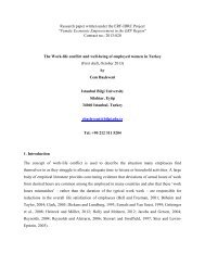
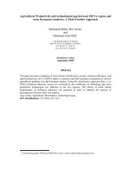
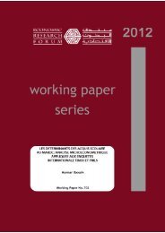
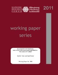
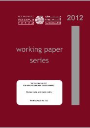
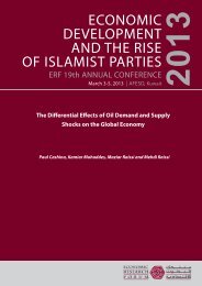
4. Poverty Mapping ResultsThis section presents the results of the two-step small area estimation methodology. Theresults of the first-step, the least squares estimates of the cluster-level equation of log percapita consumption using the HIECS data, are presented in Table 1. The model goodness offit measure (R2=0.9177) is high. It explains more than 91 percent of the variation in clusterlevelper capita consumption.9 The results of this table confirm our expectation thathousehold members’ enrolment rates and employment status, and household head's educationlevel and employment stability are significantly correlated with poverty.10 Also, asexpected, a large group of the household durables is a good predictor of poverty level.Cluster-level average possession of a car, refrigerator, VCR, satellite dish and personalcomputer appears to be associated with higher level of per capita consumption. Moreover,localities in the governorates of Alexandria, Port Said, Suez, Dumyat and South Sinai are lesslikely to be poor.Our poverty mapping exercise provides villages/shiakha-level, district-level, governoratelevel,and urban/rural-level poverty ranking—according to the predicted RPCC. Figure 1presents the full national-level distribution of village/shiakha RPCC in Egypt. Figures 2 and3 are examples of the within-governorate and within-district spatial distribution of RPCC.The poorest the locality the darker it is represented on the maps. These figures confirm thatpoverty is spatially distributed in Egypt. It is clear from Figure 1 that poor localities aremostly widespread in Upper Egypt, particularly in the Suhag, Assiut, Beni Suef, Fayoum andQina governorates.Table 2 presents the Census-based governorate-level predictions of RPCC. On thegovernorate-level, South Sinai and Port Said have the highest RPCC, while Suhag appears tobe the poorest governorate. Table 3 and Figure 4 summarize the distribution of poorest andrichest villages/shiakhas in Egypt according to their predicted RPCC by governorate. Table 3shows the governorates that have localities within the poorest 100, poorest 1000, and richest1000 localities. The poorest 50 villages in Egypt are mainly in the governorates of Suhag (33villages) and Assiut (14 villages). Marsa Matrouh, North Sinai and Beni Suef join these twogovernorates in the category of the poorest 100 villages. The table confirms that the poorestlocalities in Egypt are predominantly in Upper Egypt.According to the village/shiakha-level predicted RPCC results (not shown here), the poorestvillage/shiakha and poorest district in Egypt are in the governorate of Suhag. AwlaadShaluul (in the district of Suhag) is the poorest village and the district of Dar al-Salam is thepoorest district nationwide. In contrast, although in Table 2 the governorate of Cairo isranked the sixth according to the governorate-level predicted RPCC, the richest localitynationwide in Egypt is in Cairo: Al-Gabalaaya shiakha (in Al-Zamalik district) is the richestvillage/shiakha in Egypt and Al-Zamalik is the richest district.Figure 2 presents both the national-level ranking (left map) and the within-governorate-levelranking (right map) of the poorest governorate, Suhag. The national-level ranking map,which is just a zoomed-in version of Figure 1, shows all Suhag as one dark spot. On the rightside map, darker spots (or localities falling in the lowest quintile of the PRCC distribution)are quite dispersed all over Suhag; but are, relatively, more concentrated around the South-9For simplicity, from this section onwards, the paper refers to “localities with lower average per capitaconsumption” as “poorest localities”. However, the reader should be aware that poverty is not only a functionof average consumption but also the distribution of consumption.10The results of this step should be interpreted with caution. As mentioned above, the estimated coefficientsmay be biased and inconsistent, since some of the explanatory variables are endogenous to the poverty status.However, as discussed above, this problem is less of a concern in the context of the present analysis.6

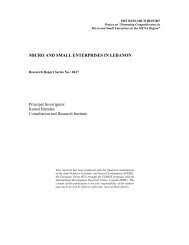
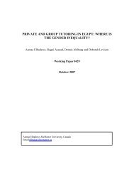
East part of the governorate where Dar al-Salam district falls. A closer view of the district ofDar al-Salam is shown in Figure 3. The national-, governorate-, and district-levels ranking ofDar al-Salam are demonstrated in this figure. On the district-level ranking map of Dar al-Salam, four areas appear to particularly fall in the bottom quintiles of the RPCC, which arethe City of Dar al-Salaam, and the three villages of al-Naghaameesh, al-Balaabeesh al-Mustagida, and Awlaad Saalam Bahari.It is clear form Table 3 that none of the Lower Egypt localities appears among the bottom100 category. The poorest locality in Lower Egypt is ranked the 237 th , which is the village ofKafr 'Abdallah 'Azeeza (Minya al-Qamh district) in Sharkia. Moreover, the poorest localitiesin Egypt are predominantly rural. Only three urban neighborhoods (shiakhas) are rankedamong the bottom 100 localities in Egypt: two shiakhas in Assiut (al-Madaabigh wa Gebaanaal-Muslimeen and al-Ghoneim City), and one in Suhag (Dar al-Salaam City). Also, only 26urban neighborhoods show up among the bottom 1000 localities in Egypt. In comparison,about 62 percent of the richest localities in Egypt are urban neighborhoods.Figure 4 shows the distribution of the poorest 1000 and richest 1000 localities in Egypt, as apercentage of the total number of localities within each governorate. The governoratesranking in this figure differs from that presented in Table 3. The table shows Cairo as thegovernorate with the highest incidence of top income localities, and Suhag with the highestincidence of low income localities. Looking at the percentage of richest localities withineach governorate (Figure 4), Dumiat comes first and Suhag and Assiut come last. About 99percent of villages/shiakhas in Dumiat appear among the richest 1000 localities in Egypt, andnone of its localities appears among the poorest 1000 localities. In each of Suhag and Assiut,about 90 percent of the localities are among the poorest 1000 category, while less than onepercent belongs to the richest group.Due to the unavailability of the household-level data, we are unable to provide reliableestimates of local-level inequality measures. Nevertheless, to get an idea of the withingovernorateinequality, we sketch in Figure 5 the distribution of village/shiakha predictedRPCC by governorate. In most of the governorates, the distribution of RPCC appears to bestrongly concentrated around the governorate median with quite a few outliers. Thevillage/shiakha RPCC distribution appears to be, relatively, more widely spread in Red Sea,North Sinai, and the Metropolitan governorates. Outliers are, particularly more obviouslydispersed away from the distribution mean in Alexandria, Cairo, and Giza. In contrast,outliers are very limited in Qina, Aswan, and Luxor. Surprisingly, almost all of the outliersappearing in the figure are at the top of the governorates PRCC distribution. Based on theresults presented in Table 2 and Figure 4, we cannot reject the often highlighted presumptionthat inequality is less severe in poor communities. To accurately test this presumptionhousehold-level data is needed (see Minot et al. (2003) and Simler and Nhate (2003) formeasurements and tests of inequality using household-level data)5. Conclusions, limitations and future workThis study produces a finely detailed poverty map for Egypt, which goes substantially furtherin terms of geographic disaggregation than previously produced poverty estimates. Thepaper combines the full coverage of the 1996 Population Census and the detailed informationon income and expenditure provided from the 1999/2000 HIECS to estimate per capitaconsumption for all localities in Egypt. Results show that poverty is spatially distributed inEgypt. Substantial disparities in the incidence of poverty exist between localities. Also, thewithin-governorate distribution of poor and rich localities varies markedly. The poorestlocalities in Egypt are predominantly rural and are mostly located in Upper Egypt. Suhag isthe poorest governorate in Egypt, and it also comprises the poorest localities nationwide.7

These results suggest that the geographical dimension of poverty should be carefullyconsidered when designing public policies and poverty alleviation programs in Egypt.However, the analysis of this paper suffers from two main problems that often face anyregression model of spatial relation. One common problem is the existence of spatialautocorrelation, which is present when the dependent variable or the error term is correlatedacross clusters. Another problem is the heteroskedasticity (different variance across clusters)of the dependent variable (see Minot et al. (2003) for details on how each of these problemsmanifests itself). The existence of these problems needs to be carefully investigated, andproper regression procedures that account for stratification and clustering should be applied.Hence, further poverty analysis research is needed in Egypt, particularly as household leveldata gets available, to produce more precise estimates of poverty and inequality at the locallevel.6.Policy ImplicationThis study produces a finely detailed poverty map for Egypt, which goes substantially furtherin terms of geographic disaggregation than previously produced poverty estimates. Thepaper combines the full coverage of the 1996 Population Census and the detailed informationon income and expenditure provided from the 1999/2000 HIECS to estimate per capitaconsumption for all localities in Egypt. Results show that poverty is spatially distributed inEgypt. Substantial disparities in the incidence of poverty exist between localities. Also, thewithin-governorate distribution of poor and rich localities varies markedly. The poorestlocalities in Egypt are predominantly rural and are mostly located in Upper Egypt. Suhag isthe poorest governorate in Egypt, and it also comprises the poorest localities nationwide.Strategic targeting of social assistance and safety net provisions is currently on the top of thepublic officials and policy makers agenda in Egypt. Maximizing the efficiency of targetingmechanisms was one of the primarily reasons of recently combining the Ministry of SocialAffairs (MOSA) and Ministry of Supply (MOS) into the Ministry of Social Solidarity (MSS).This merge is expected to more efficiently allow policy makers to pool together resources ofboth ministries when formulating social assistance strategies for vulnerable groups. Forinstance, the MOS used to apply a sort of universal non-targeted, or weakly targeted,mechanism to distribute in-kind food subsidies through either ration-cards or subsidizedinputs to bakeries. In contrast, the MOSA had a separate system through which financialcash transfers were directly made to poor families. This system was ostensibly targeted to thevery poor by means of information gathered by locally-based social workers, but was verylimited in scope and provided very meager social support to the household it reached. Theobjective of the new Ministry of Social Solidarity is to more efficiently target the resourcesavailable for subsidies so that a large proportion reaches needy households—providing themwith a more effective safety net. The MSS is proposing to use a combination of geographictargeting and proxy means tests of individual households.The existence of substantial disparities in the incidence of poverty between localities in Egyptmotivates the use of a geographic targeting mechanism when designing public policies andpoverty alleviation programs. Geographic targeting of poverty alleviation programs has anumber of advantages over universal non-targeted or self-targeting mechanisms and proxymeanstargeting approach. In a universal non-targeted program, resources (e.g. subsidies ofinferior goods) are transferred not only to the poor but also to the non-poor. Hence, despitethe low administrative cost of a non-targeted program, the total program cost can be quitehigh to achieve the same amount of social protection.On the other hand, the proxy-mean approach is based on a set of basic household-levelinformation (e.g. education levels, household structure, durable goods and access to services)8

combined into some sort of an index of social need. Though, the leakage rate of the proxymeanapproach is potentially lower than the non-targeted or self-targeted mechanism, itrequires high administrative cost and expensive regular updates. Additionally, moral hazardaffects the quality of the reported information by the household. Under this approach,households have incentives to either change their behavior to qualify for a program/subsidyor misrepresent information about themselves in order to continue being eligible for aprogram.In comparison to the universal non-targeted and the proxy-mean mechanisms, geographictargeting offers the potential for more efficient outcomes in terms of minimizing leakagerates, administrative costs, and under-coverage. Additionally, the moral hazard problem isnot an issue in a geographic targeting mechanism, since under this mechanism policy makerstarget a whole community—not a household. Thus, there would be no incentive for a singlehousehold to change behavior or distort the data in order to qualify for a subsidy. However,there might exist an incentive to move to a targeted community to reach subsidized goods orservices. Also, targeting one locality might increase the sense of inequality of distribution ofgoods and services between neighboring communities.Therefore, in a developing country like Egypt where resources are limited, both leakage andunder-coverage rates would be substantially minimized by using a detailed geographicaltargeting mechanism as the one developed in this paper. Using such a poverty mappingmechanism would allow policy makers to easily compare poverty rates acrossdistricts/villages, identify localities with a high concentration of the poor, and understand thegeographic characteristics of areas that are falling behind. Nevertheless, the efficiency ofsuch geographic targeting may be further improved if combined with a mix of a self-targetingmechanism and proxy-mean approach (such as combining geographic targeting withobservable characteristics of beneficiaries or poor communities). Such a mix of povertytargeting mechanisms would allow policy makers to tailor antipoverty programs resourcesmore effectively according to local conditions and needs of the targeted areas.Thus, the allocation of resources in Egypt should be prioritized according to the povertymapping rankings. For instance, based on the study results, the efficiency of targeting wouldbe maximized if a largest share of anti-poverty programs resources is first allocated to thepoorest localities nationwide, which are in Suhag and Assiut. These poverty alleviationprograms may take many forms. A thorough examination of the within-governorate rankingmap of Suhag reveals that the dark spots representing poor localities increase the further wemove away from the governorate capital or center cities (Madinet Suhag and Markaz Suhag),and the closer we get to the governorate borders (Dar al-Salam, Tima, Tahta, Guhayna andAl-Maragha districts). Thus, a potential poverty alleviation program could take the form ofreducing economic distance between these remote poor communities and the city centers; forexample, by allowing a better access to the public services available in the city centers.Another poverty alleviation strategy could be allocating more investments to basic servicesand infrastructure according to the needs of each community. The poverty map, developed inthis study, could also be utilized to understand the geographic distribution of those needs bymapping a mix of indicators of locality characteristics. For instance, comparing the withingovernorateranking map of Suhag and each of the within-governorate ranking of femaleilliteracy rate and household access to public water connection maps (Figure 6), it is clear thatthe poor communities tends to have higher rates of female illiteracy and lower access topublic water network. More specifically, once again, darker spots of high illiteracy rates andlow access to water connection appear more concentrated the further we move away fromMarkaz/Madinet Suhag, particularly in Dar al-Salam and the North-West border districts.9

Summing up, this discussion highlights that the efficiency of strategic targeting may bemaximized if it is based on a detailed geographic targeting mechanism combined with amechanism that carefully accounts for the characteristics of poor communities orbeneficiaries. Implementing both mechanisms would be required—either one alone may notbe sufficient—to efficiently target the poor in Egypt.10

ReferencesAstrup, C. and S. Dessus. 2001. “Targeting the Poor Beyond Gaza or the West Bank: TheGeography of Poverty on the Palestinian Territories,” ERF Working Paper 0120.Bigman, D. and H. Fofack. 2000. Geographic Targeting for Poverty Alleviation:Methodology and Application. World Bank Regional and Sectoral Studies, WashingtonDC, USA.Deaton, A. 1997. The Analysis of Household Surveys: A Microeconometric Approach toDevelopment Policy. John Hopkins University Press, Baltimore, MD.Datt, G.; and D. Jolliffe. 2005. “Poverty in Egypt: Modeling and Policy Simulations,”Economic Development and Cultural Change, Vol. 53(2): 327–346.Elbers, C., J. Lanjouw and P. Lanjouw. 2002. “Micro-Level Estimation of Welfare,” PolicyResearch Working paper 2911. Development Research Group, World Bank, Washingon,DC.El-Leithy, H. and M. Osman. 1997. “Profile and Trend of Poverty and Economic Growth inEgypt,” Egypt Human Development Report 1997. Institute of National Planning, Egypt.El-Laithy, H. and M. Lokshin. 2002. "Economic Growth and Poverty: Egypt 19995-2000,"Mimeo, Background Paper, June 2002.El-Laithy, H., M. Lokshin and A. Banerji. 2003. “Poverty and Economic Growth in Egypt,1995-2000,” Policy Research Working Paper #3068, The World Bank.Haddad, L. and A. Ahmed. 2003. “Chronic and Transitory Poverty: Evidence from Egypt,”World Development, Vol. 31(1): 71-86.Henninger, N. and M. Snel. 2002. Where are the poor? Experiences with the Developmentand Use of Poverty maps. World Research Institute, Washington. D.C. and UNEP-GRID/Arendal, Arendal, Norway.Hentschel, J., J. Lanjouw, P. Lanjouw and J. Poggi. 2000. “Combining Census and SurveyData to Trace the Spatial Dimension of Poverty: A Case Study of Ecuador,” World BankEconomic Review, Vol. 14(1): 147-165.Minot, N. 2000. “Generating Disaggregate Poverty Maps: An Application to Vietnam,”World Development, Vol. 28(2): 319-331.Minot, N. and B. Baulch. 2002. “The Spatial Distribution of Poverty in Vietnam and thePotential for Targeting,” Discussion Paper No. 42. Markets and Structural StudiesDivision, International Food Policy Research Institute, Washington D.C.Minot, N. and B. Baulch. 2005. “Poverty Mapping with Aggregate Census Data: What is theLoss in Precision?” Review of. Development Economics, Vol. 9 (1), 5–25.Minot, N., B. Baulch, and M. Epprecht. 2003. Poverty and Inequality in Vietnam: SpatialPatters and Geographic Determinants, International Food Policy Research Institute,Washington D.C. and Institute of Development Studies, University of Sussex, UnitedKingdom.11

Simler, K. and V. Nhate. 2003. Poverty , Inequality, and Geographic Targeting: Evidencefrom Small-area Estimations in Mozambique. International Food Policy ResearchInstitute, Washington DC, USA.Van de Walle, D. 1998. “Targeting Revisited,” The World bank Research Observer, Vol.13(2): 231-248.12

Figure 1 Distribution of village/shiakha predicted PCC in Egypt (national-ranking)SharkiaFayoumBeni SuefAssiutSuhagQina13

Figure 2 Distribution of village/shiakha predicted PCC in SuhagNational-RankingGovernorate-RankingTimaTahtaGuhaynaMarkazSuhagMadinetSuhagAl-MaraghaDar al-Salam14

Figure 3 Distribution of village/shiakha predicted PCC in Dar-al-Salam district inSuhagNational-Ranking15

Figure 4 Distribution of poorest 1000 and richest 1000 villages/shiakhas in Egypt bygovernorate, and their within-governorate incidenceaverage100%80%60%40%20%0%DumiatSuezCairoPort SaidAlexandriaIsmailiaNew ValleyKafr al-SheikhRed SeaKaliobiaAswanSouth SinaiGharbiaGizaTop 1000 Middle Bottom 100016

Figure 5 Distribution of predicted RPCC by governorate8000700060005000RPCC40003000200010000N =292Cairo50004000RPCC30002000N =13717978477516213223AlexandriaPort SaidSuezDumiatDakahliaSharkiaKaliobiaKafr al-Shaykh1000017

500040003000RPCC200010000N =347326469362132331693642595000GharbiaMenoufiaBehiraIsmailiaGizaBeni SuefFayoumMinyaAssiut4000RPCC30002000N =28619695221431427421SuhagQinaAswanLuxorRed SeaNew ValleyMarsa MatrouhNorth SinaiSouth Sinai1000018

Figure 6 Distribution of village/shiakha female illiteracy rate and percent ofhouseholds with public water connection in SuhagFemale Female Illiteracy Illiteracy Rate RatePublic Public Water Water Connection Connection19

Table 1 Regression results of PSU-level log per capita consumption, using HIECS dataVariables Coefficient Standard ErrorlgAvgHsz 0.553 0.922lgAvgHszSq -0.146 0.287pEldrlyMa 1.317 0.818pEldrlyFa 0.391 0.888pChilda 0.235 0.328pYoungsta -0.187 0.344pAdultFa 0.826 * 0.440RlDpRatioa -0.027 0.025UmpRatea -0.109 0.177PrmEnrRoM 0.204 ** 0.096PrmEnrRoF 0.026 0.092PIllt10Ma 0.032 0.218PIllt10Fa -0.109 0.146pUnivH18M -0.379 0.260pUnivH18F -0.196 0.263pWAgrPrM -0.569 *** 0.202pWContPrM -0.728 ** 0.313pLabor6t14M 0.230 0.214pLabor6t14F 0.248 0.340pHHYoung 9.684 7.408pHHPermF -0.016 0.195pEldrAlon 0.196 0.404pHHReadWr -0.043 0.176pHHPrimPr 0.140 0.218pHHSecond -0.083 0.186pHHAbvSec 0.010 0.290pHHUnivH 0.531 * 0.300pHHWAgrPr 0.474 * 0.277pHHWConPr 0.908 ** 0.410urb_rural 0.237 0.223Alexandria 0.067 ** 0.034Port Said 0.235 *** 0.076Suways 0.296 *** 0.063Dumyat 0.416 * 0.239Daqahliyya 0.024 0.233Sharqiyya 0.001 0.229Qalyubiyya 0.232 0.231Kafr al-Shaykh 0.327 0.233Gharbiyya 0.207 0.231Minufiyya 0.063 0.234Buhayra 0.213 0.228Ismailiyya 0.232 0.242Giza 0.112 0.231Bani Suwayf 0.035 0.240Fayyum 0.101 0.236Minya 0.243 0.238Asyut -0.018 0.234Suhag -0.085 0.232Qina 0.075 0.235Aswan 0.125 0.235Luxor 0.056 0.248Red Sea 0.308 0.27220

Table 1 Regression results of PSU-level log per capita consumption, using HIECS dataContd.Variables Coefficient Standard ErrorWadi al-gadid 0.218 0.275Marsa Matruh 0.166 0.269Shimal Sina 0.133 0.284Ganub Sina 0.586 *** 0.160urb rural × Dumyat -0.247 0.242urb rural × Daqahliyya -0.077 0.232urb rural × Sharqiyya -0.269 0.228Urb rural × Qalyubiyya -0.258 0.231Urb rural × Kafr al-Shaykh -0.252 0.235Urb rural × Gharbiyya -0.201 0.230Urb rural × Minufiyya -0.166 0.234Urb rural × Buhayra -0.276 0.230Urb rural × Ismailiyya -0.152 0.251Urb rural × Giza -0.258 0.229Urb rural × Bani Suwayf -0.186 0.239Urb rural × Fayyum -0.285 0.240Urb rural × Minya -0.192 0.239Urb rural × Asyut -0.326 0.235Urb rural × Suhag -0.221 0.231Urb rural × Qina -0.197 0.238Urb rural × Aswan -0.288 0.243Urb rural × Luxor -0.176 0.262Urb rural × Red Sea -0.147 0.307Urb rural × Wadi al-gadid -0.131 0.309Urb rural × Marsa Matruh -0.183 0.309Urb rural × Shimal Sina -0.173 0.320HHpersroom -0.085 0.060pRuralHH 0.000 0.057pUntradHH 0.321 1.536pRoomsHH 0.026 0.187pWaterPub -0.055 0.058pPrivKit 0.046 0.080pPrivToil 0.005 0.166pPrivBath 0.055 0.073pCar 0.409 ** 0.194pWashmach 0.097 0.131pFridge 0.206 * 0.114pFreeze 0.128 0.151pAC 0.077 0.175pColTV 0.075 0.170pBWTV 0.015 0.148pVCR 0.495 *** 0.119pDish 0.406 ** 0.224pPC 1.099 *** 0.293_cons 6.156 *** 0.86921

Table 2 Average predicted RPCC by governorateGovernoratesAverage predicted RPCCSouth Sinai 3224.48Port Said 2714.39Suez 2705.63Dumiat 2426.42Red Sea 2361.66Cairo 2309.63Alexandria 2223.54Ismailia 2139.90New Valley 2058.57Giza 1874.42Kaliobia 1873.15Kafr al-Shaykh 1851.60Gharbia 1829.00North Sinai 1691.02Marsa Matrouh 1673.81Aswan 1642.54Luxor 1625.61Dakahlia 1621.66Behira 1621.38Minya 1546.23Menoufia 1507.42Qina 1456.54Sharkia 1437.49Beni Suef 1326.03Fayoum 1295.34Assiut 1185.41Suhag 1164.0722

Table 3 Distribution of the poorest 100, poorest 1000, and richest 1000 villages/shiakhain Egypt by governorateBottom 100 Bottom 1000 Top 1000Governorate% of% of% ofIncidence Category Incidence CategoryCategory totaltotaltotalSuhag 61% 258 25.8% 3 0.3%Assiut 28% 232 23.2% 1 0.1%Beni Suef 4% 146 14.6% 4 0.4%North Sinai 4% 32 3.2% 11 1.1%Marsa Matrouh 3% 9 0.9% 5 0.5%Fayoum 114 11.4% 3 0.3%Qina 37 3.7% 7 0.7%Minya 20 2.0% 17 1.7%Luxor 1 0.1%Sharkia 72 7.2% 8 0.8%Suez 9 0.9%Red Sea 10 1.0%Menoufia 24 2.4% 13 1.3%Port Said 16 1.6%New Valley 1 19 1.9%South Sinai 20 2.0%Ismailia 1 0.1% 24 2.4%Dakahlia 22 2.2% 25 2.5%Aswan 2 0.2% 28 2.8%Giza 19 1.9% 39 3.9%Behira 10 1.0% 41 4.1%Kaliobia 1 0.1% 69 6.9%Gharbia 73 7.3%Dumiat 77 7.7%Kafr al-Shaykh 103 10.3%Alexandria 111 11.1%Cairo 263 26.3%% of urbanneighborhoods (shiakhas)3% 26 2.6% 619 61.9%Total 100% 1000 100% 1000 100%23

AppendixTable A1 Description of variables used in the regression analysisVariables Correlation Variable Variable DescriptionCoefficient Type1. lgAvgHsz -0.42 Continuous Log of average household size2. lgAvgHszSq Continuous Log of average household size squared3. pEldrlyMa 0.33 Continuous Percent Elderly males4. pEldrlyFa 0.17 Continuous Percent Elderly females5. pChilda -0.61 Continuous Percent children6. pYoungsta -0.57 Continuous Percent Youngsters7. pAdultFa Continuous Percent adult females8. RlDpRatioa -0.46 Continuous Real Dependency ratio9. UmpRatea 0.00 Continuous Unemployment rate10. PrmEnrRoM 0.24 Continuous Primary enrolment rate of males11. PrmEnrRoF 0.37 Continuous Primary enrolment rate of females12. PIllt10Ma -0.51 Continuous Percent illiterate males13. PIllt10Fa -0.69 Continuous Percent illiterate females14. pUnivH18M 0.78 Continuous Percent males with university education15. pUnivH18F 0.80 Continuous Percent females with university education16. pWAgrPrM -0.47 Continuous Percent male wage and unpaid family workers in agriculture in private sector17. pWContPrM -0.01 Continuous Percent male wage employees in construction in private sector18. pLabor6t14M Continuous Percent male child/adolescent labor (6-14 years)19. pLabor6t14F Continuous Percent female child/adolescent labor (6-14 years)20. pHHYoung Continuous Percent children headed households (less than 15 years old)21. pHHPermF 0.21 Continuous Percent permanent female headed households22. pEldrAlon 0.09 Continuous Percent households with an elderly living alone23. pHHReadWr 0.11 Continuous Percent household heads that can read & write24. pHHPrimPr Continuous Percent household heads with primary education25. pHHSecond Continuous Percent household heads with secondary education26. pHHAbvSec Continuous Percent household heads with above secondary education27. pHHUnivH 0.78 Continuous Percent household heads with University or higher education28. pHHWAgrPr -0.38 Continuous Percent of household heads wage employed in agriculture in private sector29. pHHWConPr -0.01 Continuous Percent of household heads wage employed in construction in private sector30. HHpersroom -0.31 Continuous Number of persons per room (density)31. pRuralHH -0.51 Continuous Percent of rural type houses32. pUntradHH -0.03 Continuous Percent of untraditional type houses33. pRoomsHH -0.22 Continuous Percent of room-type houses34. pWaterPub 0.21 Continuous Percent household connected to public water network35. pPrivKit 0.49 Continuous Percent household with private kitchen36. pPrivToil 0.42 Continuous Percent household with private Toilet37. pPrivBath 0.48 Continuous Percent household with private bath38. pCar 0.76 Continuous Percent household with a car39. pWashmach 0.44 Continuous Percent household with a washing machine(Continue)40. pFridge 0.64 Continuous Percent household with a refrigerator41. pFreeze 0.76 Continuous Percent household with a Freezer42. pAC 0.67 Continuous Percent household with an airconditioner43. pColTV 0.79 Continuous Percent household with a colored TV44. pBWTV -0.42 Continuous Percent with a black & white TV45. pVCR 0.85 Continuous Percent household with a VCR46. pDish 0.61 Continuous Percent household with a satellite dish24

Table A1 Description of variables used in the regression analysis – Contd.Variables Correlation Variable Variable DescriptionCoefficient Type47. pPC 0.65 Continuous Percent household with a personal computer48. urb_rural 0.63 Binary PSU in an urban area (rural = omitted category)49. GovernoratesBinary 26 governorate dummies (Cairo= omited category)dummies50. urban andgovernoratedummiesinteractionsBinary Interaction terms of urb_rural and governorate dummy variablesTable A2 Estimated per-capita region-specific poverty lines for 1999/2000RegionEstimated per-capitaGovernoratesregion-specific poverty linesMetropolitan 1,109 Cairo, Alexandria, Port Said, SuezLower Egypt Urban 1,015Lower Egypt Rural 978Upper Egypt Urban 1,031Upper Egypt Rural 964Frontier Urban 1,021Frontier Rural 1,049Dumiat, Dakhalia, Sharkia, Kalyoubia,Kafr El-Shaikh, Gharbia, Menoufia,Behera, IsmailaGiza, Beni-Suef, Fayoum, Menia,Assyout, Suhag, Quena, AswanRed Sea, New Valley, Matrouh, NorthSinai, South SinaiSource: El-Laithy and Lokshin (2002)25