Quantum Field Theory - Notes 1 Introduction - University of Glasgow

Quantum Field Theory - NotesChris White (University of Glasgow)AbstractThese notes are a write-up of lectures given at the RAL school for High Energy Physicists,which took place at Somerville College, Oxford in September 2010. The aim is to introduce thecanonical quantisation approach to QFT, and derive the Feynman rules for a scalar field.1 IntroductionQuantum Field Theory is a highly important cornerstone of modern physics. It underlies, forexample, the description of elementary particles i.e. the Standard Model of particle physics is aQFT. There is currently no observational evidence to suggest that QFT is insufficient in describingparticle behaviour, and indeed many theories for beyond the Standard Model physics (e.g.supersymmetry, extra dimensions) are QFTs. There are some theoretical reasons, however, forbelieving that QFT will not work at energies above the Planck scale, at which gravity becomesimportant. Aside from particle physics, QFT is also widely used in the description of condensedmatter systems, and there has been a fruitful interplay between the fields of condensed matterand high energy physics.We will see that the need for QFT arises when one tries to unify special relativity and quantummechanics, which explains why theories of use in high energy particle physics are quantumfield theories. Historically, Quantum Electrodynamics (QED) emerged as the prototype of modernQFT’s. It was developed in the late 1940s and early 1950s chiefly by Feynman, Schwingerand Tomonaga, and has the distinction of being the most accurately verified theory of all time:the anomalous magnetic dipole moment of the electron predicted by QED agrees with experimentwith a stunning accuracy of one part in 10 10 ! Since then, QED has been understood asforming part of a larger theory, the Standard Model of particle physics, which also describes theweak and strong nuclear forces. As you will learn at this school, electromagnetism and the weakinteraction can be unified into a single “electroweak” theory, and the theory of the strong forceis described by Quantum Chromodynamics (QCD). QCD has been verified in a wide range ofcontexts, albeit not as accurately as QED (due to the fact that the QED force is much weaker,allowing more accurate calculations to be carried out).As is clear from the above discussion, QFT is a type of theory, rather than a particulartheory. In this course, our aim is to introduce what a QFT is, and how to derive scattering amplitudesin perturbation theory (in the form of Feynman rules). For this purpose, it is sufficientto consider the simple example of a single, real scalar field. More physically relevant exampleswill be dealt with in the other courses. Throughout, we will follow the so-called canonicalquantisation approach to QFT, rather than the path integral approach. Although the latterapproach is more elegant, it is less easily presented in such a short course.The structure of these notes is as follows. In the rest of the introduction, we review thoseaspects of classical and quantum mechanics which are relevant in discussing QFT. In particular,we go over the Lagrangian formalism in point particle mechanics, and see how this can also beused to describe classical fields. We then look at the quantum mechanics of non-relativistic point

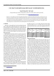
particles, and recall the properties of the quantum harmonic oscillator, which will be useful inwhat follows. We then briefly show how attempts to construct a relativistic analogue of theSchödinger equation lead to inconsistencies. Next, we discuss classical field theory, derivingthe equations of motion that a relativistic scalar field theory has to satisfy, and examining therelationship between symmetries and conservation laws. We then discuss the quantum theoryof free fields, and interpret the resulting theory in terms of particles, before showing how todescribe interactions via the S-matrix and its relation to Green’s functions. Finally, we describehow to obtain explicit results for scattering amplitudes using perturbation theory, which leads(via Wick’s theorem) to Feynman diagrams.1.1 Classical MechanicsLet us begin this little review by considering the simplest possible system in classical mechanics,a single point particle of mass m in one dimension, whose coordinate and velocity are functions oftime, x(t) and ẋ(t) = dx(t)/dt, respectively. Let the particle be exposed to a time-independentpotential V (x). It’s motion is then governed by Newton’s lawm d2 xdt 2 = −∂V ∂x= F(x), (1)where F(x) is the force exerted on the particle. Solving this equation of motion involves twointegrations, and hence two arbitrary integration constants to be fixed by initial conditions.Specifying, e.g., the position x(t 0 ) and velocity ẋ(t 0 ) of the particle at some initial time t 0completely determines its motion: knowing the initial conditions and the equations of motion,we also know the evolution of the particle at all times (provided we can solve the equations ofmotion).We can also derive the equation of motion using an entirely different approach, via theLagrangian formalism. This is perhaps more abstract than Newton’s force-based approach, butin fact is easier to generalise and technically more simple in complicated systems (such as fieldtheory!), not least because it avoids us having to think about forces at all.First, we introduce the LagrangianL(x, ẋ) = T − V = 1 2 mẋ2 − V (x), (2)which is a function of coordinates and velocities, and given by the difference between the kineticand potential energies of the particle. Next, we define the actionS =∫ t1t 0dt L(x, ẋ). (3)The equations of motion are then given by the principle of least action, which says that thetrajectory x(t) followed by the particle is precisely that such that S is extremised 1 . To verifythis in the present case, let us rederive Newton’s Second Law.First let us suppose that x(t) is indeed the trajectory that extremises the action, and thenintroduce a small perturbationx(t) → x(t) + δx(t), (4)such that the end points are fixed:x ′ (t 1 ) = x(t 1 )x ′ (t 2 ) = x(t 2 )}⇒ δx(t 1 ) = δx(t 2 ) = 0. (5)2

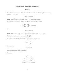
xx(t)x’(t)Figure 1: Variation of particle trajectory with identified initial and end points.tThis sends S to some S +δS, where δS = 0 if S is extremised. One may Taylor expand to giveS + δS ==∫ t2L(x + δx, ẋ + δẋ)dt, δẋ = dt 1dt δx∫ t2{L(x, ẋ) + ∂L}∂Lδx +t 1∂x ∂ẋ δẋ + . . . dt∫ t2{ ∂L∂x − d dt= S + ∂L∂ẋ δx ∣ ∣∣∣t 2t 1+t 1}∂Lδxdt, (6)∂ẋwhere we performed an integration by parts on the last term in the second line. The second andthird term in the last line are the variation of the action, δS, under variations of the trajectory,δx. The second term vanishes because of the boundary conditions for the variation, and we areleft with the third. Now the Principal of Least Action demands δS = 0. For the remainingintegral to vanish for arbitrary δx is only possible if the integrand vanishes, leaving us with the⁀Euler-Lagrange equation:∂L∂x − d ∂L= 0. (7)dt ∂ẋIf we insert the Lagrangian of our point particle, Eq. (2), into the Euler-Lagrange equation weobtain∂L∂xd ∂Ldt ∂ẋ∂V (x)= − = F∂x= d mẋ = mẍdt⇒ mẍ = F = − ∂V∂x(Newton’s law). (8)Hence, we have derived the equation of motion (the Euler-Lagrange equation) using the Principalof least Action and found it to be equivalent to Newton’s Second Law. The benefit of the formeris that it can be easily generalised to other systems in any number of dimensions, multi-particlesystems, or systems with an infinite number of degrees of freedom, such as needed for field theory.For example, a general system of point particles has a set {q i } of generalised coordinates,which may not be simple positions but also angles etc. The equations of motion are then given1 The name of the principle comes from the fact that, in most cases, S is indeed minimised.3

yd ∂L= ∂L ,dt ∂ ˙q i ∂q iby analogy with the one-dimensional case. That is, each coordinate has its own Euler-Lagrangeequation (which may nevertheless depend on the other coordinates, so that the equations ofmotion are coupled). Another advantage of the Lagrangian formalism is that the relationshipbetween symmetries and conserved quantities is readily understood - more on this later.First, let us note that there is yet another way to think about classical mechanics (that wewill see again in quantum mechanics / field theory), namely via the Hamiltonian formalism.Given a Lagrangian depending on generalised coordinates {q i }, we may define the conjugatemomentap i = ∂L∂ ˙q ie.g. in the simple one-dimensional example given above, there is a single momentum p = mẋconjugate to x. We recognise as the familiar definition of momentum, but it is not always truethat p i = m ˙q i .We may now define the HamiltonianH({q i }, {p i }) = ∑ i˙q i p i − L({q i }, { ˙q i }).As an example, consider againL = 1 2 mẋ2 − V (x).It is easy to show from the above definition thatH = 1 2 mẋ2 + V (x),which we recognise as the total energy of the system. From the definition of the Hamiltonianone may derive (problem 1.1)∂H ∂H= −ṗ i , = ẋ i ,∂q i ∂p iwhich constitute Hamilton’s equations. These are useful in proving the relation between symmetriesand conserved quantities. For example, one readily sees from the above equations thatthe momentum p i is conserved if H does not depend explicitly on q i . That is, conservationof momentum is related to invariance under spatial translations, if q i can be interpreted as asimple position coordinate.1.2 Quantum mechanicsHaving set up some basic formalism for classical mechanics, let us now move on to quantummechanics. In doing so we shall use canonical quantisation, which is historically what was usedfirst and what we shall later use to quantise fields as well. We remark, however, that one canalso quantise a theory using path integrals.Canonical quantisation consists of two steps. Firstly, the dynamical variables of a system arereplaced by operators, which we denote by a hat. Secondly, one imposes commutation relationson these operators,[ˆx i , ˆp j ] = i δ ij (9)[ˆx i , ˆx j ] = [ˆp i , ˆp j ] = 0. (10)4

The physical state of a quantum mechanical system is encoded in state vectors |ψ〉, which areelements of a Hilbert space H. The hermitian conjugate state is 〈ψ| = (|ψ〉) † , and the modulussquared of the scalar product between two states gives the probability for the system to go fromstate 1 to state 2,|〈ψ 1 |ψ 2 〉| 2 = probability for |ψ 1 〉 → |ψ 2 〉. (11)On the other hand physical observables O, i.e. measurable quantities, are given by the expectationvalues of hermitian operators, Ô = Ô† ,O = 〈ψ|Ô|ψ〉, O 12 = 〈ψ 2 |Ô|ψ 1〉. (12)Hermiticity ensures that expectation values are real, as required for measurable quantities. Dueto the probabilistic nature of quantum mechanics, expectation values correspond to statisticalaverages, or mean values, with a variance(∆O) 2 = 〈ψ|(Ô − O)2 |ψ〉 = 〈ψ|Ô2 |ψ〉 − 〈ψ|Ô|ψ〉2 . (13)An important concept in quantum mechanics is that of eigenstates of an operator, defined byÔ|ψ〉 = O|ψ〉. (14)Evidently, between eigenstates we have ∆O = 0. Examples are coordinate eigenstates, ˆx|x〉 =x|x〉, and momentum eigenstates, ˆp|p〉 = p|p〉, describing a particle at position x or withmomentum p, respectively. However, a state vector cannot be simultaneous eigenstate ofnon-commuting operators. This leads to the Heisenberg uncertainty relation for any two noncommutingoperators Â, ˆB,∆A∆B ≥ 1 2 |〈ψ|[Â, ˆB]|ψ〉|. (15)Finally, sets of eigenstates can be orthonormalized and we assume completeness, i.e. they spanthe entire Hilbert space,∫〈p ′ |p〉 = δ(p − p ′ ), 1 = d 3 p |p〉〈p|. (16)As a consequence, an arbitrary state vector can always be expanded in terms of a set of eigenstates.We may then define the position space wavefunctionso thatψ(x) = 〈x|ψ〉,∫〈ψ 1 |ψ 2 〉 = d 3 x〈ψ 1 |x〉〈x|ψ 2 〉∫= d 3 xψ1 ∗ (x)ψ 2(x). (17)Acting on the wavefunction, the explicit form of the position and momentum operators isso that the Hamiltonian operator isˆx = x, ˆp = −i∇, (18)Ĥ = ˆp22m + V (x) = ∇ 2−2 + V (x). (19)2mHaving quantised our system, we now want to describe its time evolution. This can be done indifferent “pictures”, depending on whether we consider the state vectors or the operators (orboth) to depend explicitly on t, such that expectation values remain the same. Two extremecases are those where the operators do not depend on time (the Schrödinger picture), and whenthe state vectors do not depend on time (the Heisenberg picture). We discuss these two choicesin the following sections.5

1.3 The Schrödinger pictureIn this approach state vectors are functions of time, |ψ(t)〉, while operators are time independent,∂ t Ô = 0. The time evolution of a system is described by the Schrödinger equation 2 ,i ∂ ψ(x, t) = Ĥψ(x, t). (20)∂tIf at some initial time t 0 our system is in the state Ψ(x, t 0 ), then the time dependent state vectorΨ(x, t) = e − i Ĥ(t−t0) Ψ(x, t 0 ) (21)solves the Schrödinger equation for all later times t.The expectation value of some hermitian operator Ô at a given time t is then defined as∫〈Ô〉 t = d 3 xΨ ∗ (x, t)ÔΨ(x, t), (22)and the normalisation of the wavefunction is given by∫d 3 xΨ ∗ (x, t)Ψ(x, t) = 〈1〉 t . (23)Since Ψ ∗ Ψ is positive, it is natural to interpret it as the probability density for finding a particleat position x. Furthermore one can derive a conserved current j, as well as a continuity equationby consideringΨ ∗ × (Schr.Eq.) − Ψ × (Schr.Eq.) ∗ . (24)The continuity equation reads∂ρ = −∇ · j (25)∂twhere the density ρ and the current j are given byρ = Ψ ∗ Ψ (positive), (26)j = 2im (Ψ∗ ∇Ψ − (∇Ψ ∗ )Ψ) (real). (27)Now that we have derived the continuity equation let us discuss the probability interpretationof Quantum Mechanics in more detail. Consider a finite volume V with boundary S. Theintegrated continuity equation is∫V∂ρ∂t d3 x == −∫−∫VS∇ · j d 3 xj · dS (28)where in the last line we have used Gauss’s theorem. Using Eq.(23) the left-hand side can berewritten and we obtain∫∂∂t 〈1〉 t = − j · dS = 0. (29)SIn other words, provided that j = 0 everywhere at the boundary S, we find that the timederivative of 〈1〉 t vanishes. Since 〈1〉 t represents the total probability for finding the particleanywhere inside the volume V , we conclude that this probability must be conserved: particlescannot be created or destroyed in our theory. Non-relativistic Quantum Mechanics thus providesa consistent formalism to describe a single particle. The quantity Ψ(x, t) is interpreted as a oneparticlewave function.2 Note that the Hamiltonian could itself have some time dependence in general, even in the Schrödinger picture, ifthe potential of a system depends on time. Here we assume this is not the case.6

1.4 The Heisenberg pictureHere the situation is the opposite to that in the Schrödinger picture, with the state vectorsregarded as constant, ∂ t |Ψ H 〉 = 0, and operators which carry the time dependence, ÔH(t). Thisis the concept which later generalises most readily to field theory. We make use of the solutionEq. (21) to the Schrödinger equation in order to define a Heisenberg state vector throughΨ(x, t) = e − i Ĥ(t−t0) Ψ(x, t 0 ) ≡ e − i Ĥ(t−t0) Ψ H (x), (30)i.e. Ψ H (x) = Ψ(x, t 0 ). In other words, the Schrödinger vector at some time t 0 is defined tobe equivalent to the Heisenberg vector, and the solution to the Schrödinger equation providesthe transformation law between the two for all times. This transformation of course leaves thephysics, i.e. expectation values, invariant,with〈Ψ(t)|Ô|Ψ(t)〉 = 〈Ψ(t 0)|e i Ĥ(t−t0) Ôe − i Ĥ(t−t0) |Ψ(t 0 )〉 = 〈Ψ H |ÔH(t)|Ψ H 〉, (31)Ô H (t) = e i Ĥ(t−t0) Ôe − i Ĥ(t−t0) . (32)From this last equation it is now easy to derive the equivalent of the Schrödinger equation forthe Heisenberg picture, the Heisenberg equation of motion for operators:i dÔH(t)dt= [ÔH, Ĥ]. (33)Note that all commutation relations, like Eq. (9), with time dependent operators are now intendedto be valid for all times. Substituting ˆx, ˆp for Ô into the Heisenberg equation readilyleads todˆx idtdˆp idt= ∂Ĥ∂ˆp i,= − ∂Ĥ∂ˆx i, (34)the quantum mechanical equivalent of the Hamilton equations of classical mechanics.1.5 The quantum harmonic oscillatorBecause of similar structures later in quantum field theory, it is instructive to also briefly recallthe harmonic oscillator in one dimension. Its Hamiltonian is given byĤ(ˆx, ˆp) = 1 ( ) ˆp22 m + mω2ˆx 2 . (35)Employing the canonical formalism we have just set up, we easily identify the momentumoperator to be ˆp(t) = m∂ tˆx(t), and from the Hamilton equations we find the equation of motionto be ∂t 2ˆx = −ω2ˆx, which has the well known plane wave solution ˆx ∼ exp iωt.An alternative path useful for later field theory applications is to introduce new operators,expressed in terms of the old ones,(√â = √ 1√ ) (√ mω 12 ˆx + i mω ˆp , â † = √ 1√ )mω 12 ˆx − i mω ˆp . (36)Using the commutation relation for ˆx, ˆp, one readily derives (see the preschool problems)[â, â † ] = 1, [Ĥ, â] = −ωâ, [Ĥ, ↠] = ωâ † . (37)7

With the help of these the Hamiltonian can be rewritten in terms of the new operators:Ĥ = 1 2 ω ( â † â + ââ †) (= â † â + 1 )ω. (38)2With this form of the Hamiltonian it is easy to construct a complete basis of energy eigenstates|n〉,Ĥ|n〉 = E n |n〉. (39)Using the above commutation relations, one findsand thereforeâ † Ĥ|n〉 = (Ĥ↠− ωâ † )|n〉 = E n â † |n〉, (40)Ĥâ † |n〉 = (E n + ω)â † |n〉. (41)Thus, the state â † |n〉 has energy E n + ω, so that â † may be regarded as a “creation operator”for a quantum with energy ω. Along the same lines one finds that â|n〉 has energy E n − ω,and â is an “annihilation operator”.Let us introduce a vacuum state |0〉 with no quanta excited, for which â|n〉 = 0, becausethere cannot be any negative energy states. Acting with the Hamiltonian on that state we findĤ|0〉 = ω/2, (42)i.e. the quantum mechanical vacuum has a non-zero energy, known as vacuum oscillation or zeropoint energy. Acting with a creation operator onto the vacuum state one easily finds the statewith one quantum excited, and this can be repeated n times to get|1〉 = â † |0〉 , E 1 = (1 + 1 2 )ω, . . .|n〉 = √ â†|n − 1〉 = √ 1 (â † ) n |0〉 , E n = (n + 1 )ω. (43)n n! 2The root of the factorial is there to normalise all eigenstates to one. Finally, the number operatorˆN = â † â returns the number of quanta in a given energy eigenstate,ˆN|n〉 = n|n〉. (44)1.6 Relativistic Quantum MechanicsSo far we have only considered non-relativistic particles. In this section, we see what happenswhen we try to formulate a relativistic analogue of the Schrödinger equation. First, note thatwe can derive the non-relativistic equation starting from the energy relationE = p2+ V (x) (45)2mand replacing variables by their appropriate operators acting on a position space wavefunctionψ(x, t)E → i ∂ , p → −i∇, x → x (46)∂tto give []− 2∂ψ(x, t)2m ∇2 + V (x) ψ(x, t) = i . (47)∂t8

As we have already seen, there is a corresponding positive definite probability densitywith corresponding currentρ = |ψ(x, t)| 2 ≥ 0, (48)j = 2im (ψ∗ ∇ψ − (∇ψ ∗ )ψ). (49)Can we also make a relativistic equation? By analogy with the above, we may start withthe relativistic energy relationE 2 = c 2 p 2 + m 2 c 4 , (50)and making the appropriate operator replacements leads to the equation( 1 ∂ 2c 2 ∂t 2 − ∇2 + m2 c 2 ) 2 φ(x, t) (51)for some wavefunction φ(x, t). This is the Klein-Gordon equation, and one may try to form aprobability density and current, as in the non-relativistic case. Firstly, one notes that to satisfyrelativistic invariance, the probability density should be the zeroth component of a 4-vectorj µ = (ρ,j) satisfying∂ µ j µ = 0. (52)In fact, one findsρ = i (φ ∗ ∂φ )2m ∂t − φ∂φ∗ , (53)∂twith j given as before. This is not positive definite! That is, this may (and will) become negativein general, so we cannot interpret this as the probability density of a single particle.There is another problem with the Klein-Gordon equation as it stands, that is perhaps lessabstract to appreciate. The relativistic energy relation givesE = ± √ c 2 p 2 + m 2 c 4 , (54)and thus one has positive and negative energy solutions. For a free particle, one could restrictto having positive energy states only. However, an interacting particle may exchange energywith its environment, and there is nothing to stop it cascading down to energy states of moreand more negative energy, thus emitting infinite amounts of energy.We conclude that the Klein-Gordon equation does not make sense as a consistent quantumtheory of a single particle. We thus need a different approach in unifying special relativity andquantum mechanics. This, as we will see, is QFT, in which we will be able to reinterpret theKlein-Gordon function as a field φ(x, t) describing many particles.From now on, it will be extremely convenient to work in natural units, in which one sets = c = 1. The correct factors can always be reinstated by dimensional analysis. In these units,the Klein-Gordon equation becomes(□ + m 2 )φ(x, t) = 0, (55)where□ = ∂ µ ∂ µ = ∂∂t 2 − ∇2 . (56)9

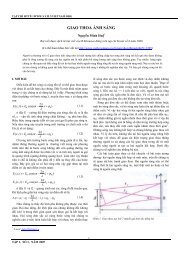
Figure 2: System of masses m joined by springs (of constant k), whose longitudinal displacementsare {f i }, and whose separation at rest is δx.2 Classical Field TheoryIn the previous section, we have seen how to describe point particles, both classically and quantummechanically. In this section, we discuss classical field theory, as a precursor to consideringquantum fields. A field associates a mathematical object (e.g. scalar, vector, tensor, spinor...)with every point in spacetime. Examples are the temperature distribution in a room (a scalarfield), or the E and B fields in electromagnetism (vector fields). Just as point particles canbe described by Lagrangians, so can fields, although it is more natural to think in terms ofLagrangian densities.2.1 Example: Model of an Elastic RodLet us consider a particular example, namely a set of point masses connected together by springs,as shown in figure 2. Assume the masses m are equal, as also are the force constants of thesprings k. Furthermore, we assume that the masses may move only longitudinally, where the i thdisplacement is f i , and that the separation of adjacent masses is δx when all f i are zero. Thissystem is an approximation to an elastic rod, with a displacement field f(x, t). To see what thisfield theory looks like, we may first write the total kinetic and potential energies asT = ∑ i12 m ˙ f 2 i ,V = ∑ i12 k(f i+1 − f i ) 2 (57)respectively, where we have used Hooke’s Law for the potential energy. Thus, the Lagrangian isL = T − V = ∑ [ 12 m f ˙ i 2 − 1 ]2 k(f i+1 − f i ) 2 . (58)iClearly this system becomes a better approximation to an elastic rod as the continuum limit isapproached, in which the number of masses N → ∞ and the separation δx → 0. We can thenrewrite the Lagrangian asL = ∑ [1( m)δx f ˙i 2 − 1 ( ) ] 22 δx 2 (kδx) fi+1 − f i. (59)δxiWe may recogniselim m/δx = ρ (60)δx→010

as the density of the rod, and also define the tensionκ = lim kδx. (61)δx→0Furthermore, the position index i gets replaced by the continuous variable x, and one hasf i+1 − f ilim =δx→0 δx∂f(x, t). (62)∂xFinally, the sum over i becomes an integral so that the continuum Lagrangian is∫ [1L = dx2 ρ f(x, ˙ t) 2 − 1 ( ) ] 2 ∂f2 κ . (63)∂xThis is the Lagrangian for the displacement field f(x, t). It depends on a function of f and f ˙which is integrated over all space coordinates (in this case there is only one, the position alongthe rod). We may therefore write the Lagrangian manifestly aswhere L is the Lagrangian density∫L =dxL[f(x, t), ˙ f(x, t)], (64)L[f(x, t), f(x, ˙ t)] = 1 2 ρ f ˙2(x, t) − 1 ( ) 2 ∂f2 κ . (65)∂xIt is perhaps clear from the above example that for any field, there will always be an integrationover all space dimensions, and thus it is more natural to think about the Lagrangian densityrather than the Lagrangian itself. Indeed, we may construct the following dictionary betweenquantities in point particle mechanics, and corresponding field theory quantities (which may ormay not be helpful to you in remembering the differences between particles and fields...!).Classical Mechanics:Classical Field Theory:x(t) −→ φ(x, t) (66)ẋ(t) −→ ˙φ(x, t)Index i −→ Coordinate x (67)L(x, ẋ) −→ L[φ, ˙φ] (68)Note that the action for the above field theory is given, as usual, by the integral of the Lagrangian:∫ ∫ ∫S = dtL = dt dxL[f, f]. ˙(69)2.2 Relativistic FieldsIn the previous section we saw how fields can be described using Lagrangian densities, andillustrated this with a non-relativistic example. Rather than derive the field equations for thiscase, we do this explicitly here for relativistic theories, which we will be concerned with for therest of the course (and, indeed, the school).In special relativity, coordinates are combined into four-vectors, x µ = (t, x i ) or x = (t,x),whose length x 2 = t 2 − x 2 is invariant under Lorentz transformationsx ′µ = Λ µ ν x ν . (70)11

A general function transforms as f(x) → f ′ (x ′ ), i.e. both the function and its argument transform.A Lorentz scalar is a function φ(x) which at any given point in space-time will have thesame amplitude, regardless of which inertial frame it is observed in. Consider a space-time pointgiven by x in the unprimed frame, and x ′ (x) in the primed frame, where the function x ′ (x) canbe derived from eq. (70). Observers in both the primed and unprimed frames will see the sameamplitude φ(x), although an observer in the primed frame will prefer to express this in termsof his or her own coordinate system x ′ , hence will seeφ(x) = φ(x(x ′ )) = φ ′ (x ′ ), (71)where the latter equality defines φ ′ .Equation (71) defines the transformation law for a Lorentz scalar. A vector function transformsasV ′µ (x ′ ) = Λ µ ν V ν (x). (72)We will work in particular with ∂ µ φ(x), where x ≡ x µ denotes the 4-position. Note in particularthat( ) 2 ∂φ(∂ µ φ)(∂ µ φ) = − ∇φ · ∇φ∂t∂ µ ∂ µ φ = ∂2 φ∂t 2 − ∇2 φ.In general, a relativistically invariant scalar field theory has action∫S = d 4 xL[φ, ∂ µ φ], (73)where∫∫d 4 x ≡dt d 3 x, (74)and L is the appropriate Lagrangian density. We can find the equations of motion satisfied bythe field φ using, as in point particle mechanics, the principle of least action. The field theoryform of this is that the field φ(x) is such that the action of eq. (73) is extremised. Assumingφ(x) is indeed such a field, we may introduce a small perturbationwhich correspondingly perturbs the action according to∫S → S + δS = d 4 xφ(x) → φ(x) + δφ(x), (75)[L(φ, ∂ µ φ) + ∂L∂φ δφ +]∂L∂(∂ µ φ) δ(∂ µφ) . (76)Recognising the first term as the unperturbed action, one thus finds∫ [ ∂LδS = d 4 x∂φ δφ + ∂L ]∂(∂ µ φ) δ(∂ µφ)[ ∫ [ ( )]∂L∂L ∂L=∂(∂ µ φ)]boundaryδφ + d 4 x∂φ − ∂ µ δφ,∂(∂ µ φ)where we have integrated by parts in the second line. Assuming the fields die away at infinityso that δφ = 0 at the boundary of spacetime, the principle of least action δS = 0 implies( ) ∂L∂ µ = ∂L∂(∂ µ φ) ∂φ . (77)12

This is the Euler-Lagrange field equation. It tells us, given a particular Lagrangian density(which defines a particular field theory) the classical equation of motion which must be satisfiedby the field φ. As a specific example, let us consider the Lagrangian densityL = 1 2 (∂ µφ)(∂ µ φ) − 1 2 m2 φ 2 , (78)from which one finds∂L∂(∂ µ φ) = ∂µ φ,so that the Euler-Lagrange equation gives∂L∂φ = −m2 φ, (79)∂ µ ∂ µ φ + m 2 φ = (□ + m 2 )φ(x) = 0. (80)This is the Klein-Gordon equation! The above Lagrangian density thus corresponds to theclassical field theory of a Klein-Gordon field. We see in particular that the coefficient of thequadratic term in the Lagrangian can be interpreted as the mass.By analogy with point particle mechanics, one can define a canonical momentum field conjugateto φ:π(x) = ∂L . (81)∂ ˙φThen one can define the Hamiltonian densityH[φ, π] = π ˙φ − L, (82)such that∫H =d 3 x H(π, φ) (83)is the Hamiltonian (total energy carried by the field). For example, the Klein-Gordon field hasconjugate momentum π = ˙φ, and Hamiltonian densityH = 1 2[π 2 (x) + (∇φ) 2 + m 2 φ 2] . (84)2.3 Plane wave solutions to the Klein-Gordon equationLet us consider real solutions to Eq. (80), characterised by φ ∗ (x) = φ(x). To find them we tryan ansatz of plane wavesφ(x) ∝ e i(k0 t−k·x) . (85)The Klein-Gordon equation is satisfied if (k 0 ) 2 − k 2 = m 2 so thatDefining the energy aswe obtain two types of solution which readk 0 = ± √ k 2 + m 2 . (86)E(k) = √ k 2 + m 2 > 0, (87)φ + (x) ∝ e i(E(k)t−k·x) , φ − (x) ∝ e −i(E(k)t−k·x) . (88)We may interpret these as positive and negative energy solutions, such that it does not matterwhich branch of the square root we take in eq. (87) (it is conventional, however, to define energyas a positive quantity). The general solution is a superposition of φ + and φ − . UsingE(k)t − k · x = k µ k µ = k µ k µ = k · x (89)13

this solution reads∫φ(x) =d 3 k(2π) 3 2E(k)(e ik·x α ∗ (k) + e −ik·x α(k) ) , (90)where α(k) is an arbitrary complex coefficient. Note that the coefficients of the positive andnegative exponentials are related by complex conjugation. This ensures that the field φ(x) isreal (as can be easily verified from eq. (90)), consistent with the Lagrangian we wrote down.Such a field has applications in e.g. the description of neutral mesons. We can also write downa Klein-Gordon Lagrangian for a complex field φ. This is really two independent fields (i.e. φand φ ∗ ), and thus can be used to describe a system of two particles (e.g. charged meson pairs).To simplify the discussion in this course, we will explicitly consider the real Klein-Gordon field.Note that the factors of 2 and π in eq. (90) are conventional, and the inverse power of the energyis such that the measure of integration is Lorentz invariant (problem 2.1), so that the wholesolution is written in a manifestly Lorentz invariant way.2.4 Symmetries and Conservation LawsAs was the case in point particle mechanics, one may relate symmetries of the Lagrangiandensity to conserved quantities in field theory. For example, consider the invariance of L underspace-time translationsx µ → x µ + ǫ µ , (91)where ǫ µ is constant. Under such a transformation one hasL(x µ + ǫ µ ) = L(x µ ) + ǫ µ ∂ µ L(x µ ) + . . . (92)φ(x µ + ǫ µ ) = φ(x µ ) + ǫ µ ∂ µ φ(x µ ) + . . . (93)∂ ν φ(x µ + ǫ µ ) = ∂ ν φ(x µ ) + ǫ µ ∂ µ ∂ ν φ(x µ ) + . . . , (94)where we have used Taylor’s theorem. But if L does not explicitly depend on x µ (i.e. onlythrough φ and ∂ µ φ) then one hasL(x µ + ǫ µ ) = L[φ(x µ + ǫ µ ), ∂ ν φ(x µ + ǫ µ )]= L + ∂L∂φ δφ +(95)∂L∂(∂ ν φ) δ(∂ νφ) + . . . (96)= L + ∂L∂φ ǫµ ∂ µ φ +∂L∂(∂ ν φ) ǫµ ∂ µ ∂ ν φ + . . . , (97)where we have used the fact that δφ = ǫ µ ∂ µ φ in the third line, and all functions on the righthandside are evaluated at x µ . One may replace ∂L/∂φ by the LHS of the Euler-Lagrangeequation to getL(x µ + ǫ µ ∂L) = L + ∂ ν∂(∂ ν φ) ǫµ ∂ µ φ +∂L∂(∂ ν φ) ǫµ ∂ µ ∂ ν φ + . . .[ ] ∂L= L + ∂ ν∂(∂ ν φ) ∂ µφ ǫ µ , (98)and equating this with the alternative expression above, one finds[ ] ∂L∂ ν∂(∂ ν φ) ∂ µφ ǫ µ = ǫ µ ∂ µ L. (99)14

If this is true for all ǫ µ , then one haswhereΘ νµ =∂ ν Θ νµ = 0, (100)∂L∂(∂ ν φ) ∂ µφ − g µν L (101)is the energy-momentum tensor. We can see how this name arises by considering the componentsexplicitly, for the case of the Klein Gordon field. One then findsΘ 00 = ∂L∂ ˙φ˙φ − g 00 L = π ˙φ − L = H, (102)Θ 0j = ∂L∂ ˙φ ∂ jφ − g 0j L = π∂ j φ (j = 1 . . .3). (103)One then sees that Θ 00 is the energy density carried by the field. Its conservation can then beshown by considering∫∫∂d 3 xΘ 00 = d 3 x∂ 0 Θ 00∂t VV∫∫= d 3 x∂ j Θ j0 = dS j · Θ 0j = 0, (104)Vwhere we have used Eq. (100) in the second line. The Hamiltonian density is a conservedquantity, provided that there is no energy flow through the surface S which encloses the volumeV . In a similar manner one can show that the 3-momentum p j , which is related to Θ 0j , isconserved as well. It is then useful to define a conserved energy-momentum four-vector∫P µ = d 3 x Θ 0µ . (105)In analogy to point particle mechanics, we thus see that invariances of the Lagrangian densitycorrespond to conservation laws. An entirely analogous procedure leads to conserved quantitieslike angular mometum and spin. Furthermore one can study so-called internal symmetries,i.e. ones which are not related to coordinate but other transformations. Examples are conservationof all kinds of charges, isospin, etc.We have thus established the Lagrange-Hamilton formalism for classical field theory: we derivedthe equation of motion (Euler-Lagrange equation) from the Lagrangian and introduced theconjugate momentum. We then defined the Hamiltonian (density) and considered conservationlaws by studying the energy-momentum tensor Θ µν .3 Quantum Field Theory: Free Fields3.1 Canonical Field QuantisationIn the previous sections we have reviewed the classical and quantum mechanics of point particles,and also classical field theory. We used the canonical quantisation procedure in discussing quantummechanics, whereby classical variables are replaced by operators, which have non-trivialcommutation relations. In this section, we see how to apply this procedure to fields, taking theexplicit example of the Klein-Gordon field discussed previously. This is, as yet, a non-interactingfield theory, and we will discuss how to deal with interactions later on in the course.The Klein-Gordon Lagrangian density has the formSL = 1 2 ∂µ φ∂ µ φ − 1 2 m2 φ 2 . (106)15

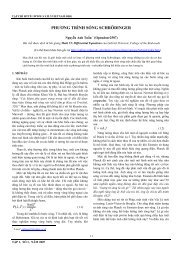
time(x − y) 2 > 0, time-like(x − y) 2 = 0, light-likey(x − y) 2 < 0, space-likespaceFigure 3: The light cone about y. Events occurring at points x and y are said to be time-like(space-like) if x is inside (outside) the light cone about y.We have seen that in field theory the field φ(x) plays the role of the coordinates in ordinary pointparticle mechanics, and we defined a canonically conjugate momentum, π(x) = ∂L/∂ ˙φ = ˙φ(x).We then continue the analogy to point mechanics through the quantisation procedure, i.e. wenow take our canonical variables to be operators,φ(x) → ˆφ(x), π(x) → ˆπ(x). (107)Next we impose equal-time commutation relations on them,[ˆφ(x, t), ˆπ(y, t)]= iδ 3 (x − y), (108)[ˆφ(x, t), ˆφ(y, t)]= [ˆπ(x, t), ˆπ(y, t)] = 0. (109)As in the case of quantum mechanics, the canonical variables commute among themselves, butnot the canonical coordinate and momentum with each other. Note that the commutationrelation is entirely analogous to the quantum mechanical case. There would be an , if it hadn’tbeen set to one earlier, and the delta-function accounts for the fact that we are dealing withfields. It is zero if the fields are evaluated at different space-time points.After quantisation, our fields have turned into field operators. Note that within the relativisticformulation they depend on time, and hence they are Heisenberg operators.In the previous paragraph we have formulated commutation relations for fields evaluated atequal time, which is clearly a special case when considering fields at general x, y. The reasonhas to do with maintaining causality in a relativistic theory. Let us recall the light cone aboutan event at y, as in Fig. 3. One important postulate of special relativity states that no signaland no interaction can travel faster than the speed of light. This has important consequencesabout the way in which different events can affect each other. For instance, two events whichare characterised by space-time points x µ and y µ are said to be causal if the distance (x − y) 2is time-like, i.e. (x − y) 2 > 0. By contrast, two events characterised by a space-like separation,i.e. (x − y) 2 < 0, cannot affect each other, since the point x is not contained inside the lightcone about y.In non-relativistic Quantum Mechanics the commutation relations among operators indicatewhether precise and independent measurements of the corresponding observables can be made.If the commutator does not vanish, then a measurement of one observable affects that of the16

other. From the above it is then clear that the issue of causality must be incorporated intothe commutation relations of the relativistic version of our quantum theory: whether or notindependent and precise measurements of two observables can be made depends also on theseparation of the 4-vectors characterising the points at which these measurements occur. Clearly,events with space-like separations cannot affect each other, and hence all fields must commute,]][ˆφ(x), ˆφ(y) = [ˆπ(x), ˆπ(y)] =[ˆφ(x), ˆπ(y) = 0 for (x − y) 2 < 0. (110)This condition is sometimes called micro-causality. Writing out the four-components of the timeinterval, we see that as long as |t ′ − t| < |x − y|, the commutator vanishes in a finite interval|t ′ − t|. It also vanishes for t ′ = t, as long as x ≠ y. Only if the fields are evaluated at anequal space-time point can they affect each other, which leads to the equal-time commutationrelations above. They can also affect each other everywhere within the light cone, i.e. for timelikeintervals. It is not hard to show that in this case (e.g. problem 3.1)] [ˆφ(x), ˆφ(y) = [ˆπ(x), ˆπ(y)] = 0, for (x − y) 2 > 0 (111)] [ˆφ(x), ˆπ(y) = i ∫d 3 p(2 (2π) 3 e ip·(x−y) + e −ip·(x−y)) . (112)n.b. since the 4-vector dot product p · (x − y) depends on p 0 = √ p 2 + m 2 , one cannot triviallycarry out the integrals over d 3 p here.3.2 Creation and annihilation operatorsAfter quantisation, the Klein-Gordon equation we derived earlier turns into an equation foroperators. For its solution we simply promote the classical plane wave solution, Eq. (90), tooperator status,∫dˆφ(x) 3 k (=eik·xâ †(2π) 3 (k) + e −ik·x â(k) ) . (113)2E(k)Note that the complex conjugation of the Fourier coefficient turned into hermitian conjugationfor an operator.Let us now solve for the operator coefficients of the positive and negative energy solutions.In order to do so, we invert the Fourier integrals for the field and its time derivative,∫d 3 x ˆφ(x, t)e ikx = 1 [â(k)+ â † (k)e 2ik0x0] , (114)2E∫d 3 x ˙ˆφ(x, t)eikx= − i [â(k)− â † (k)e 2ik0x0] , (115)2and then build the linear combination iE(k)(114)−(115) to find∫d 3 x[iE(k)ˆφ(x, t) − ˙ˆφ(x,]t) e ikx = iâ(k), (116)Following a similar procedure for â † (k), and using ˆπ(x) = ˙ˆφ(x) we find∫ []â(k) = d 3 x E(k)ˆφ(x, t) + iˆπ(x, t) e ikx , (117)∫ []â † (k) = d 3 x E(k)ˆφ(x, t) − iˆπ(x, t) e −ikx . (118)Note that, as Fourier coefficients, these operators do not depend on time, even though theright hand side does contain time variables. Having expressions in terms of the canonical17

field variables ˆφ(x), ˆπ(x), we can now evaluate the commutators for the Fourier coefficients.Expanding everything out and using the commutation relations Eq. (109), we find[â†(k 1 ), â † (k 2 ) ] = 0 (119)[â(k 1 ), â(k 2 )] = 0 (120)[â(k1), â † (k 2 ) ] = (2π) 3 2E(k 1 )δ 3 (k 1 − k 2 ) (121)We easily recognise these for every k to correspond to the commutation relations for the harmonicoscillator, Eq. (37). This motivates us to also express the Hamiltonian and the energy momentumfour-vector of our quantum field theory in terms of these operators. To do this, first note thatthe Hamiltonian is given by the integral of the Hamiltonian density (eq. (84)) over all space.One may then substitute eq. (113) to yield (see the problem sheet)∫Ĥ = 1 2ˆP = 1 ∫2d 3 k(2π) 3 2E(k) E(k)( â † (k)â(k) + â(k)â † (k) ) , (122)d 3 k(2π) 3 2E(k) k( â † (k)â(k) + â(k)â † (k) ) . (123)We thus find that the Hamiltonian and the momentum operator are nothing but a continuoussum of excitation energies/momenta of one-dimensional harmonic oscillators! After a minute ofthought this is not so surprising. We expanded the solution of the Klein-Gordon equation into asuperposition of plane waves with momenta k. But of course a plane wave solution with energyE(k) is also the solution to a one-dimensional harmonic oscillator with the same energy. Hence,our free scalar field is simply a collection of infinitely many harmonic oscillators distributedover the whole energy/momentum range. These energies sum up to that of the entire system.We have thus reduced the problem of handling our field theory to oscillator algebra. From theharmonic oscillator we know already how to construct a complete basis of energy eigenstates,and thanks to the analogy of the previous section we can take this over to our quantum fieldtheory.3.3 Energy of the vacuum state and renormalisationIn complete analogy we begin again with the postulate of a vacuum state |0〉 with norm one,which is annihilated by the action of the operator a,〈0|0〉 = 1, â(k)|0〉 = 0 for all k. (124)Let us next evaluate the energy of this vacuum state, by taking the expectation value of theHamiltonian,E 0 = 〈0|Ĥ|0〉 = 1 ∫d 3 k2 (2π) 3 2E(k) E(k){ 〈0|â † (k)â(k)|0〉 + 〈0|â(k)â † (k)|0〉 } . (125)The first term in curly brackets vanishes, since a annihilates the vacuum. The second can berewritten asâ(k)â † (k)|0〉 = {[ â(k), â † (k) ] + â † (k)â(k) } |0〉. (126)It is now the second term which vanishes, whereas the first can be replaced by the value of thecommutator. Thus we obtainE 0 = 〈0|Ĥ|0〉 = δ3 (0) 1 ∫d 3 k E(k) = δ 3 (0) 1 ∫d 3 k √ k222 + m 2 = ∞, (127)which means that the energy of the ground state is infinite! This result seems rather paradoxical,but it can be understood again in terms of the harmonic oscillator. Recall that the simple18

quantum mechanical oscillator has a finite zero-point energy. As we have seen above, our fieldtheory corresponds to an infinite collection of harmonic oscillators, i.e. the vacuum receives aninfinite number of zero point contributions, and its energy thus diverges.This is the first of frequent occurrences of infinities in quantum field theory. Fortunately, itis not too hard to work around this particular one. Firstly, we note that nowhere in nature canwe observe absolute values of energy, all we can measure are energy differences relative to somereference scale, at best the one of the vacuum state, |0〉. In this case it does not really matterwhat the energy of the vacuum is. This then allows us to redefine the energy scale, by alwayssubtracting the (infinite) vacuum energy from any energy we compute. This process is called“renormalisation”.We then define the renormalised vacuum energy to be zero, and take it to be the expectationvalue of a renormalised Hamiltonian,E R 0 ≡ 〈0|ĤR |0〉 = 0. (128)According to this recipe, the renormalised Hamiltonian is our original one, minus the (unrenormalised)vacuum energy,Ĥ R = Ĥ − E 0 (129)= 1 ∫d 3 k2 (2π) 3 2E(k) E(k){ â † (k)â(k) + â(k)â † (k) − 〈0|â † (k)â(k) + â(k)â † (k)|0〉 }= 1 ∫d 3 k2 (2π) 3 2E(k) E(k){ 2â † (k)â(k) + [ â(k), â † (k) ] − 〈0| [ â(k), â † (k) ] |0〉 } . (130)Here the subtraction of the vacuum energy is shown explicitly, and we can rewrite is as∫Ĥ R d 3 p=(2π) 3 2E(p) E(p)↠(p)â(p)+ 1 ∫d 3 p2 (2π) 3 2E(p) E(p){[ â(p), â † (p) ] − 〈0| [ â(p), â † (p) ] |0〉 } .∫d 3 p=(2π) 3 2E(p) E(p)↠(p)â(p) + Ĥvac (131)The operator Ĥvac ensures that the vacuum energy is properly subtracted: if |ψ〉 and |ψ ′ 〉 denotearbitrary N-particle states, then one can convince oneself that 〈ψ ′ |Ĥvac |ψ〉 = 0. In particularwe now find that〈0|ĤR |0〉 = 0, (132)as we wanted. A simple way to automatise the removal of the vacuum contribution is to introducenormal ordering. Normal ordering means that all annihilation operators appear to the right ofany creation operator. The notation is: ââ † : = â † â, (133)i.e. the normal-ordered operators are enclosed within colons. For instance(â†(p)â(p) + â(p)â † (p) ) : = â † (p)â(p). (134): 1 2It is important to keep in mind that â and â † always commute inside : · · · :. This is true for anarbitrary string of â and â † . With this definition we can write the normal-ordered Hamiltonianas: Ĥ : = : 1 2∫=∫d 3 p(2π) 3 2E(p) E(p)( â † (p)â(p) + â(p)â † (p) ) :d 3 p(2π) 3 2E(p) E(p)↠(p)â(p), (135)19

and thus have the relationHence, we find thatĤ R =: Ĥ : +Ĥvac . (136)〈ψ ′ | : Ĥ : |ψ〉 = 〈ψ′ |ĤR |ψ〉, (137)and, in particular, 〈0| : Ĥ : |0〉 = 0. The normal ordered Hamiltonian thus produces a renormalised,sensible result for the vacuum energy.3.4 Fock space and ParticlesAfter this lengthy grappling with the vacuum state, we can continue to construct our basis ofstates in analogy to the harmonic oscillator, making use of the commutation relations for theoperators â, â † . In particular, we define the state |k〉 to be the one obtained by acting with theoperator a † (k) on the vacuum,|k〉 = â † (k)|0〉. (138)Using the commutator, its norm is found to be〈k|k ′ 〉 = 〈0|â(k)â † (k ′ )|0〉 = 〈0|[â(k), â † (k ′ )]|0〉 + 〈0|â † (k ′ )a(k)|0〉 (139)= (2π) 3 2E(k)δ 3 (k − k ′ ), (140)since the last term in the first line vanishes (â(k) acting on the vacuum). Next we compute theenergy of this state, making use of the normal ordered Hamiltonian,∫: Ĥ : |k〉 = d 3 k ′(2π) 3 2E(k ′ ) E(k′ )â † (k ′ )â(k ′ )â † (k)|0〉 (141)and similarly one finds=∫d 3 k ′(2π) 3 2E(k ′ ) E(k′ )(2π) 3 2E(k)δ(k − k ′ )â † (k)|0〉 (142)= E(k)â † (k)|0〉 = E(k)|k〉, (143): ˆP : |k〉 = k|k〉. (144)Observing that the normal ordering did its job and we obtain renormalised, finite results, wemay now interpret the state |k〉. It is a one-particle state for a relativistic particle of mass m andmomentum k, since acting on it with the energy-momentum operator returns the relativistic oneparticle energy-momentum dispersion relation, E(k) = √ k 2 + m 2 . The a † (k), a(k) are creationand annihilation operators for particles of momentum k.In analogy to the harmonic oscillator, the procedure can be continued to higher states. Oneeasily checks that (problem 3.4): ˆP µ : â † (k 2 )â † (k 1 )|0〉 = (k µ 1 + kµ 2 )↠(k 2 )â † (k 1 )|0〉, (145)and so the state|k 2 ,k 1 〉 = 1 √2!â † (k 2 )â † (k 1 )|0〉 (146)is a two-particle state (the factorial is there to have it normalised in the same way as theone-particle state), and so on for higher Fock states.At long last we can now see how the field in our free quantum field theory is related toparticles. A particle of momentum k corresponds to an excited Fourier mode of a field. Sincethe field is a superpositon of all possible Fourier modes, one field is enough to describe all possibleconfigurations representing one or many particles of the same kind in any desired momentumstate.20

There are some rather profound ideas here about how nature works at fundamental scales.In classical physics we have matter particles, and forces which act on those particles. Theseforces can be represented by fields, such that fields and particles are distinct concepts. In nonrelativisticquantum mechanics, one unifies the concept of waves and particles (particles canhave wave-like characteristics), but fields are still distinct (e.g. one may quantise a particle inan electromagnetic field in QM, provided the latter is treated classically). Taking into accountthe effects of relativity for both particles and fields, one finds in QFT that all particles areexcitation quanta of fields. That is, the concepts of field and particle are no longer distinct, butactually manifestations of the same thing, namely quantum fields. In this sense, QFT is morefundamental than either of its preceding theories. Each force field and each matter field haveparticles associated with it.Returning to our theory for the free Klein-Gordon field, let us investigate what happensunder interchange of the two particles. Since [â † (k 1 ), â † (k 2 )] = 0 for all k 1 ,k 2 , we see that|k 2 ,k 1 〉 = |k 1 ,k 2 〉, (147)and hence the state is symmetric under interchange of the two particles. Thus, the particlesdescribed by the scalar field are bosons.Finally we complete the analogy to the harmonic oscillator by introducing a number operator∫ˆN(k) = â † (k)â(k), ˆN = d 3 k â † (k)â(k), (148)which gives us the number of bosons described by a particular Fock state,ˆN |0〉 = 0, ˆN |k〉 = |k〉, ˆN |k1 . . .k n 〉 = n|k 1 . . .k n 〉. (149)Of course the normal-ordered Hamiltonian can now simply be given in terms of this operator,∫: Ĥ := d 3 k(2π) 3 2E(k) E(k) ˆN(k), (150)i.e. when acting on a Fock state it simply sums up the energies of the individual particles togive: Ĥ : |k 1 . . .k n 〉 = (E(k 1 ) + . . . E(k n )) |k 1 . . .k n 〉. (151)This concludes the quantisation of our free scalar field theory. We have followed the canonicalquantisation procedure familiar from quantum mechanics. Due to the infinite number ofdegrees of freedom, we encountered a divergent vacuum energy, which we had to renormalise.The renormalised Hamiltonian and the Fock states that we constructed describe free relativistic,uncharged spin zero particles of mass m, such as neutral pions, for example.If we want to describe charged pions as well, we need to introduce complex scalar fields,the real and imaginary parts being necessary to describe opposite charges. For particles withspin we need still more degrees of freedom and use vector or spinor fields, which have theappropriate rotation and Lorentz transformation properties. For fermion fields (which satisfythe Dirac equation rather than the Klein-Gordon equation), one finds that the condition of apositive-definite energy density requires that one impose anti-commutation relations rather thancommutation relations. This in turn implies that multiparticle states are antisymmetric underinterchange of identical fermions, which we recognise as the Pauli exclusion principle. Thus, notonly does QFT provide a consistent theory of relativistic multiparticle systems; it also allowsus to “derive” the Pauli principle, which is put in by hand in non-relativistic quantum mechanics.More details on vector and spinor fields can be found in the other courses at this school.Here, we continue to restrict our attention to scalar fields, so as to more clearly illustrate whathappens when interactions are present.21

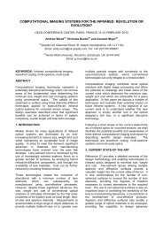
4 Quantum Field Theory: Interacting FieldsSo far we have seen how to quantise the Klein-Gordon Lagrangian, and seen that this describesfree scalar particles. For interesting physics, however, we need to know how to describe interactions,which lead to nontrivial scattering processes. This is the subject of this section.From now on we shall always discuss quantised real scalar fields. It is then convenient to dropthe “hats” on the operators that we have considered up to now. Interactions can be describedby adding a term L int to the Lagrangian density, so that the full result L is given bywhereL = L 0 + L int (152)L 0 = 1 2 ∂ µφ∂ µ φ − 1 2 m2 φ 2 (153)is the free Lagrangian density discussed before. The Hamiltonian density of the interaction isrelated to L int simply byH int = H − H 0 , (154)where H 0 is the free Hamiltonian. If the interaction Lagrangian only depends on φ (we willconsider such a case later in the course), one hasH int = −L int , (155)as can be easily shown from the definition above. We shall leave the details of L int unspecifiedfor the moment. What we will be concerned with mostly are scattering processes, in which twoinitial particles with momenta p 1 and p 2 scatter, thereby producing a number of particles in thefinal state, characterised by momenta k 1 , . . .,k n . This is schematically shown in Fig. 4. Ourtask is to find a description of such a scattering process in terms of the underlying quantumfield theory.p 1k 2p 2k 1k nFigure 4: Scattering of two initial particles with momenta p 1 and p 2 into n particles with momentak 1 ,...,k n in the final state.4.1 The S-matrixThe timescales over which interactions happen are extremely short. The scattering (interaction)process takes place during a short interval around some particular time t with −∞ ≪ t ≪ ∞.Long before t, the incoming particles evolve independently and freely. They are described by afield operator φ in defined throughlim φ(x) = φ in(x), (156)t→−∞22

which acts on a corresponding basis of |in〉 states. Long after the collision the particles in thefinal state evolve again like in the free theory, and the corresponding operator islim φ(x) = φ out(x), (157)t→+∞acting on states |out〉. The fields φ in , φ out are the asymptotic limits of the Heisenberg operatorφ. They both satisfy the free Klein-Gordon equation, i.e.(□ + m 2 )φ in (x) = 0, (□ + m 2 )φ out (x) = 0. (158)Operators describing free fields can be expressed as a superposition of plane waves (see Eq. (113)).Thus, for φ in we have∫d 3 k()φ in (x) =(2π) 3 e ik·x a † in2E(k)(k) + e−ik·x a in (k) , (159)with an entirely analogous expression for φ out (x). Note that the operators a † and a also carrysubscripts “in” and “out”.The above discussion assumes that the interaction is such that we can talk about free particlesat asymptotic times t → ±∞ i.e. that the interaction is only present at intermediate times.This is not always a reasonable assumption e.g. it does not encompass the phenomenon ofbound states, in which incident particles form a composite object at late times, which no longerconsists of free particles. Nevertheless, the assumption will indeed allow us to discuss scatteringprocesses, which is the aim of this course. Note that we can only talk about well-defined particlestates at t → ±∞ (the states labelled by “in” and “out” above), as only at these times do wehave a free theory, and thus know what the spectrum of states is (using the methods of section3). At general times t, the interaction is present, and it is not possible in general to solve forthe states of the quantum field theory. Remarkably, we will end up seeing that we can ignore allthe complicated stuff at intermediate times, and solve for scattering probabilities using purelythe properties of the asymptotic fields.At the asymptotic times t = ±∞, we can use the creation operators a † in and a† out to buildup Fock states from the vacuum. For instancea † in (p 1)a † in (p 2)|0〉 = |p 1 ,p 2 ; in〉, (160)a † out(k 1 ) · · · a † out(k n )|0〉 = |k 1 , . . . ,k n ; out〉. (161)We must now distinguish between Fock states generated by a † in and a† out, and therefore we havelabelled the Fock states accordingly. In eqs. (160) and (161) we have assumed that there is astable and unique vacuum state of the free theory (the vacuum at general times t will be thatof the full interacting theory, and thus differ from this in general):|0〉 = |0; in〉 = |0; out〉. (162)Mathematically speaking, the a † in ’s and a† out ’s generate two different bases of the Fock space.Since the physics that we want to describe must be independent of the choice of basis, expectationvalues expressed in terms of “in” and “out” operators and states must satisfy〈in| φ in (x) |in〉 = 〈out| φ out (x) |out〉. (163)Here |in〉 and |out〉 denote generic “in” and “out” states. We can relate the two bases byintroducing a unitary operator S such thatφ in (x) = S φ out (x)S † (164)|in〉 = S |out〉, |out〉 = S † |in〉, S † S = 1. (165)23

S is called the S-matrix or S-operator. Note that the plane wave solutions of φ in and φ out alsoimply thata † in = S a† out S † , â in = S â out S † . (166)By comparing “in” with “out” states one can extract information about the interaction – this isthe very essence of detector experiments, where one tries to infer the nature of the interaction bystudying the products of the scattering of particles that have been collided with known energies.As we will see below, this information is contained in the elements of the S-matrix.By contrast, in the absence of any interaction, i.e. for L int = 0 the distinction between φ inand φ out is not necessary. They can thus be identified, and then the relation between differentbases of the Fock space becomes trivial, S = 1, as one would expect.What we are ultimately interested in are transition amplitudes between an initial state i of,say, two particles of momenta p 1 ,p 2 , and a final state f, for instance n particles of unequalmomenta. The transition amplitude is then given by〈f, out| i, in〉 = 〈f, out| S |i, out〉 = 〈f, in| S |i, in〉 ≡ S fi . (167)The S-matrix element S fi therefore describes the transition amplitude for the scattering processin question. The scattering cross section, which is a measurable quantity, is then proportionalto |S fi | 2 . All information about the scattering is thus encoded in the S-matrix, which musttherefore be closely related to the interaction Hamiltonian density H int . However, before we tryto derive the relation between S and H int we have to take a slight detour.4.2 More on time evolution: Dirac pictureThe operators φ(x, t) and π(x, t) which we have encountered are Heisenberg fields and thustime-dependent. The state vectors are time-independent in the sense that they do not satisfy anon-trivial equation of motion. Nevertheless, state vectors in the Heisenberg picture can carry atime label. For instance, the “in”-states of the previous subsection are defined at t = −∞. Therelation of the Heisenberg operator φ H (x) with its counterpart φ S in the Schrödinger picture isgiven byφ H (x, t) = e iHt φ S e −iHt , H = H 0 + H int , (168)Note that this relation involves the full Hamiltonian H = H 0 + H int in the interacting theory.We have so far found solutions to the Klein-Gordon equation in the free theory, and so we knowhow to handle time evolution in this case. However, in the interacting case the Klein-Gordonequation has an extra term,(□ + m 2 )φ(x) + δV int(φ)= 0, (169)δφdue to the potential of the interactions. Apart from very special cases of this potential, the equationcannot be solved anymore in closed form, and thus we no longer know the time evolution.It is therefore useful to introduce a new quantum picture for the interacting theory, in whichthe time dependence is governed by H 0 only. This is the so-called Dirac or Interaction picture.The relation between fields in the Interaction picture, φ I , and in the Schrödinger picture, φ S ,is given byφ I (x, t) = e iH0t φ S e −iH0t . (170)At t = −∞ the interaction vanishes, i.e. H int = 0, and hence the fields in the Interaction andHeisenberg pictures are identical, i.e. φ H (x, t) = φ I (x, t) for t → −∞. The relation betweenφ H and φ I can be worked out easily:φ H (x, t)= e iHt φ S e −iHt= e iHt e −iH0t e iH0t φ S e −iH0t e iH0t e −iHt} {{ }φ I(x,t)= U −1 (t)φ I (x, t)U(t), (171)24

where we have introduced the unitary operator U(t)U(t) = e iH0t e −iHt , U † U = 1. (172)The field φ H (x, t) contains the information about the interaction, since it evolves over time withthe full Hamiltonian. In order to describe the “in” and “out” field operators, we can now makethe following identifications:t → −∞ : φ in (x, t) = φ I (x, t) = φ H (x, t), (173)t → +∞ : φ out (x, t) = φ H (x, t). (174)Furthermore, since the fields φ I evolve over time with the free Hamiltonian H 0 , they always actin the basis of “in” vectors, such thatφ in (x, t) = φ I (x, t), −∞ < t < ∞. (175)The relation between φ I and φ H at any time t is given byAs t → ∞ the identifications of eqs. (174) and (175) yieldφ I (x, t) = U(t)φ H (x, t)U −1 (t). (176)φ in = U(∞)φ out U † (∞). (177)From the definition of the S-matrix, Eq. (164) we then read off thatlim U(t) = S. (178)t→∞We have thus derived a formal expression for the S-matrix in terms of the operator U(t), whichtells us how operators and state vectors deviate from the free theory at time t, measured relativeto t 0 = −∞, i.e. long before the interaction process.An important boundary condition for U(t) islim U(t) = 1. (179)t→−∞What we mean here is the following: the operator U actually describes the evolution relative tosome initial time t 0 , which we will normally suppress, i.e. we write U(t) instead of U(t, t 0 ). Weregard t 0 merely as a time label and fix it at −∞, where the interaction vanishes. Equation (179)then simply states that U becomes unity as t → t 0 , which means that in this limit there is nodistinction between Heisenberg and Dirac fields.Using the definition of U(t), Eq.(172), it is an easy exercise to derive the equation of motionfor U(t):i d dt U(t) = H int(t)U(t), H int (t) = e iH0t H int e −iH0t . (180)The time-dependent operator H int (t) is defined in the interaction picture, and depends on thefields φ in , π in in the “in” basis. Let us now solve the equation of motion for U(t) with theboundary condition lim U(t) = 1. Integrating Eq.(180) givest→−∞∫ t∫dtU(t 1 )dt 1 = −i H int (t 1 )U(t 1 )dt 1dt 1−∞U(t) − U(−∞) =⇒ U(t) =−i1 − i25−∞∫ t−∞∫ t−∞H int (t 1 )U(t 1 )dt 1H int (t 1 )U(t 1 )dt 1 . (181)

The right-hand side still depends on U, but we can substitute our new expression for U(t) intothe integrand, which givesU(t)∫ t= 1 − i= 1 − i−∞∫ t−∞{ ∫ t1H int (t 1 ) 1 − iH int (t 1 )dt 1 −−∞∫ t−∞H int (t 2 )U(t 2 )dt 2}dt 1dt 1 H int (t 1 )∫ t1−∞dt 2 H int (t 2 )U(t 2 ), (182)where t 2 < t 1 < t. This procedure can be iterated further, so that the nth term in the sum is(−i) n ∫ t−∞dt 1∫ t1−∞∫ tn−1dt 2 · · · dt n H int (t 1 )H int (t 2 ) · · · H int (t n ). (183)−∞This iterative solution could be written in much more compact form, were it not for the fact thatthe upper integration bounds were all different, and that the ordering t n < t n−1 < . . . < t 1 < thad to be obeyed. Time ordering is an important issue, since one has to ensure that theinteraction Hamiltonians act at the proper time, thereby ensuring the causality of the theory.By introducing the time-ordered product of operators, one can use a compact notation, suchthat the resulting expressions still obey causality. The time-ordered product of two fields φ(t 1 )and φ(t 2 ) is defined as{ φ(t1 )φ(t 2 ) t 1 > t 2T {φ(t 1 )φ(t 2 )} =φ(t 2 )φ(t 1 ) t 1 < t 2≡ θ(t 1 − t 2 )φ(t 1 )φ(t 2 ) + θ(t 2 − t 1 )φ(t 2 )φ(t 1 ), (184)where θ denotes the step function. The generalisation to products of n operators is obvious.Using time ordering for the nth term of Eq.(183) we obtain(−i) nn!n∏i=1∫ t−∞dt i T {H int (t 1 )H int (t 2 ) · · · H int (t n )} . (185)Here we have replaced each upper limit of integration with t. Each specific ordering in the timeorderedproduct gives a term identical to eq. (183), where applying the T operator correspondsto setting the upper limit of integration to the relevant t i in each integral. However, we haveovercounted by a factor n!, corresponding to the number of ways of ordering the fields in thetime ordered product. Thus one must divide by n! as shown. We may recognise eq. (185) as thenth term in the series expansion of an exponential, and thus can finally rewrite the solution forU(t) in compact form aswhere the “T” in front ensures the correct time ordering.4.3 S-matrix and Green’s functions{ ∫ t}U(t) = T exp −i H int (t ′ )dt ′ , (186)−∞The S-matrix, which relates the “in” and “out” fields before and after the scattering process,can be written asS = 1 + iT, (187)where T is commonly called the T-matrix. The fact that S contains the unit operator means thatalso the case where none of the particles scatter is encoded in S. On the other hand, the nontrivialcase is described by the T-matrix, and this is what we are interested in. So far we have26

derived an expression for the S-matrix in terms of the interaction Hamiltonian, and we coulduse this in principle to calculate scattering processes. However, there is a slight complicationowing to the fact that the vacuum of the free theory is not the same as the true vacuum ofthe full, interacting theory. Instead, we will follow the approach of Lehmann, Symanzik andZimmerman, which relates the S-matrix to n-point Green’s functionsG n (x 1 , . . . x n ) = 〈0|T(φ(x 1 )...φ(x n ))|0〉 (188)i.e. vacuum expectation values of Heisenberg fields. We will see later how to calculate these interms of vacuum expectation values of “in” fields (i.e. in the free theory).In order to relate S-matrix elements to Green’s functions, we have to express the “in/out”-states in terms of creation operators a † in/outand the vacuum, then express the creation operatorsby the fields φ in/out , and finally use the time evolution to connect those with the fields φ in ourLagrangian.Let us consider again the scattering process depicted in Fig. 4. The S-matrix element in thiscase is〈〉∣S fi = k 1 ,k 2 , . . .,k n ; out∣p 1 ,p 2 ; in〈〉∣= k 1 ,k 2 , . . .,k n ; out∣a † in (p ∣1) ∣p 2 ; in , (189)where a † in is the creation operator pertaining to the “in” field φ in. Our task is now to expressa † in in terms of φ in, and repeat this procedure for all other momenta labelling our Fock states.The following identities will prove useful∫a † (p) = i d 3 x {( ∂ 0 e −iq·x) φ(x) − e −iq·x (∂ 0 φ(x)) }∫≡ −i∫â(p) = −i d 3 x {( ∂ 0 e iq·x) φ(x) − e iq·x (∂ 0 φ(x)) }∫≡ id 3 ←→−iq·xxe ∂ 0 φ(x), (190)d 3 ←→iq·xxe ∂ 0 φ(x). (191)The S-matrix element can then be rewritten as∫S fi = −i d 3 ←→〉∣ ∣x 1 e −ip1·x1 ∂0〈k 1 , . . .,k n ; out∣φ in (x 1 ) ∣p 2 ; in∫= −i lim d 3 ←→〉∣ ∣x 1 e −ip1·x1 ∂0〈k 1 , . . . ,k n ; out∣φ(x 1 ) ∣p 2 ; in , (192)t 1→−∞where in the last line we have used Eq.(156) to replace φ in by φ. We can now rewrite lim t1→−∞using the following identity, which holds for an arbitrary, differentiable function f(t), whoselimit t → ±∞ exists:∫ +∞lim f(t) = lim f(t) −t→−∞ t→+∞−∞dfdt. (193)dtThe S-matrix element then reads∫S fi = −i lim d 3 ←→〉∣ ∣x 1 e −ip1·x1 ∂0〈k 1 , . . . ,k n ; out∣φ(x 1 ) ∣p 2 ; int 1→+∞∫ +∞{∫∂+i dt 1 d 3 ←→∣ ∣x 1 e −ip1·x1 ∂0〈k 1 , . . .,k n ; out∣φ(x 1 ) ∣p 2 ; in〉 } . (194)∂t 1−∞27

The first term in this expression involves lim t1→+∞ φ = φ out , which gives rise to a contribution〈〉∣∝ k 1 , . . . ,k n ; out∣a † ∣out(p 1 ) ∣p 2 ; in . (195)This is non-zero only if p 1 is equal to one of k 1 , . . . ,k n . This, however, means that the particlewith momentum p 1 does not scatter, and hence the first term does not contribute to the T-matrix of Eq.(187). We are then left with the following expression for S fi :∫S fi = −i d 4 ∣ {(x 1〈k 1 , . . .,k n ; out∣∂ 0 ∂0 e −ip1·x1) φ(x 1 ) − e −ip1·x1 (∂ 0 φ(x 1 )) }∣ 〉∣ ∣p2 ; in . (196)The time derivatives in the integrand can be worked out:∂ 0{(∂0 e −ip1·x1) φ(x 1 ) − e −ip1·x1 (∂ 0 φ(x 1 )) }= − [E(p 1 )] 2 e −ip1·x1 φ(x 1 ) − e −ip1·x1 ∂ 2 0 φ(x 1)= − {(( −∇ 2 + m 2) e −ip1·x1 ) φ(x 1 ) + e −ip1·x1 ∂ 2 0 φ(x 1 ) } , (197)where we have used that −∇ 2 e −ip1·x1 = p 2 1 e−ip1·x1 . For the S-matrix element one obtains∫S fi = i d 4 x 1 e〈k −ip1·x1 1 , . . .,k n ; out∣ ( ∂0 2 − ∇2 + m 2) 〉∣φ(x 1 ) ∣p 2 ; in∫= i d 4 x 1 e ( −ip1·x1 □ x1 + m 2) 〈 〉∣ ∣k 1 , . . .,k n ; out∣φ(x 1 ) ∣p 2 ; in , (198)where we have used integration by parts twice so that ∇ 2 acts on φ(x 1 ) rather than on e −ip1·x1 .What we have obtained after this rather lengthy step of algebra is an expression in which the(Heisenberg) field operator is sandwiched between Fock states, one of which has been reducedto a one-particle state. We can now successively eliminate all momentum variables from theFock states, by repeating the procedure for the momentum p 2 , as well as the n momenta of the“out” state. The final expression for S fi is∫ ∫ ∫ ∫S fi = (i) n+2 d 4 x 1 d 4 x 2 d 4 y 1 · · · d 4 y n e (−ip1·x1−ip2·x2+ik1·y1+···+ikn·yn)× ( □ x1 + m 2)( □ x2 + m 2) ( □ y1 + m 2) · · · (□yn + m 2)〈〉∣∣× 0; out∣T {φ(y 1 ) · · · φ(y n )φ(x 1 )φ(x 2 )} ∣0; in , (199)where the time-ordering inside the vacuum expectation value (VEV) ensures that causalityis obeyed. The above expression is known as the Lehmann-Symanzik-Zimmermann (LSZ)reduction formula. It relates the formal definition of the scattering amplitude to a vacuumexpectation value of time-ordered fields. Since the vacuum is uniquely the same for “in/out”,the VEV in the LSZ formula for the scattering of two initial particles into n particles in thefinal state is recognised as the (n + 2)-point Green’s function:〈〉∣∣G n+2 (y 1 , y 2 , . . .,y n , x 1 , x 2 ) = 0∣T {φ(y 1 ) · · · φ(y n )φ(x 1 )φ(x 2 )} ∣0 . (200)You will note that we still have not calculated or evaluated anything, but merely rewritten theexpression for the scattering matrix elements. Nevertheless, the LSZ formula is of tremendousimportance and a central piece of QFT. It provides the link between fields in the Lagrangian andthe scattering amplitude Sfi 2 , which yields the cross section, measurable in an experiment. Upto here no assumptions or approximations have been made, so this connection between physicsand formalism is rather tight. It also illustrates a profound phenomenon of QFT and particlephysics: the scattering properties of particles, in other words their interactions, are encoded inthe vacuum structure, i.e. the vacuum is non-trivial!28

4.4 How to compute Green’s functionsOf course, in order to calculate cross sections, we need to compute the Green’s functions. Alas,for any physically interesting and interacting theory this cannot be done exactly, contrary tothe free theory discussed earlier. Instead, approximation methods have to be used in order tosimplify the calculation, while hopefully still giving reliable results. Or one reformulates theentire QFT as a lattice field theory, which in principle allows to compute Green’s functionswithout any approximations (in practice this still turns out to be a difficult task for physicallyrelevant systems). This is what many theorists do for a living. But the formalism stands,and if there are discrepancies between theory and experiments, one “only” needs to check theaccuracy with which the Green’s functions have been calculated or measured, before approvingor discarding a particular Lagrangian.In the next section we shall discuss how to compute the Green’s function of scalar field theoryin perturbation theory. Before we can tackle the actual computation, we must take a furtherstep. Let us consider the n-point Green’s functionG n (x 1 , . . . , x n ) = 〈0 |T {φ(x 1 ) · · · φ(x n )}| 0〉. (201)The fields φ which appear in this expression are Heisenberg fields, whose time evolution isgoverned by the full Hamiltonian H 0 + H int . In particular, the φ’s are not the φ in ’s. We knowhow to handle the latter, because they correspond to a free field theory, but not the former,whose time evolution is governed by the interacting theory, whose solutions we do not know.Let us thus start to isolate the dependence of the fields on the interaction Hamiltonian. Recallthe relation between the Heisenberg fields φ(t) and the “in”-fields 3φ(t) = U −1 (t)φ in (t)U(t). (202)We now assume that the fields are properly time-ordered, i.e. t 1 > t 2 > . . . > t n , so that we canforget about writing T(· · ·) everywhere. After inserting Eq.(202) into the definition of G n oneobtainsG n = 〈 0 ∣ ∣ U −1 (t 1 )φ in (t 1 )U(t 1 )U −1 (t 2 )φ in (t 2 )U(t 2 ) · · ·× U −1 (t n )φ in (t n )U(t n ) ∣ ∣ 0〉. (203)Now we introduce another time label t such that t ≫ t 1 and −t ≪ t 1 . For the n-point functionwe now obtain〈{∣G n = 0∣U −1 (t) U(t)U −1 (t 1 )φ in (t 1 )U(t 1 )U −1 (t 2 )φ in (t 2 )U(t 2 ) · · ·}〉× U −1 (t n )φ in (t n )U(t n )U −1 ∣(−t) U(−t) ∣0 . (204)The expression in curly braces is now time-ordered by construction. An important observationat this point is that it involves pairs of U and its inverse, for instanceU(t)U −1 (t 1 ) ≡ U(t, t 1 ). (205)One can easily convince oneself that U(t, t 1 ) provides the net time evolution from t 1 to t. Wecan now write G n as〈{}〉∣G n = 0∣U −1 ∣(t)T φ in (t 1 ) · · ·φ in (t n )U(t, t 1 )U(t 1 , t 2 ) · · · U(t n , −t) U(−t) ∣0 , (206)} {{ }U(t, −t)3 Here and in the following we suppress the spatial argument of the fields for the sake of brevity.29

where we have used the fact that we may commute the U operators within the time-orderedproduct. Let us now take t → ∞. The relation between U(t) and the S-matrix Eq.(178), aswell as the boundary condition Eq.(179) tell us thatlim U(−t) = 1, limt→∞U(t, −t) = S, (207)t→∞which can be inserted into the above expression. We still have to work out the meaning of〈0|U −1 (∞) in the expression for G n . In a paper by Gell-Mann and Low it was argued that thetime evolution operator must leave the vacuum invariant (up to a phase), which justifies theansatz〈0|U −1 (∞) = K〈0|, (208)with K being the phase 4 . Multiplying this relation with |0〉 from the right givesFurthermore, Gell-Mann and Low showed thatwhich implies〈0|U −1 (∞)|0〉 = K〈0|0〉 = K. (209)〈0|U −1 (∞)|0〉 =K =After inserting all these relations into the expression for G n we obtainThe S-matrix is given by1〈0|U(∞)|0〉 , (210)1〈0|S|0〉 . (211)G n (x 1 , . . .,x n ) = 〈0| T {φ in(x 1 ) · · · φ in (x n )S} |0〉. (212)〈0|S|0〉S = T exp{ ∫ +∞}−i H int (t)dt , H int = H int (φ in , π in ), (213)−∞and thus we have finally succeeded in expressing the n-point Green’s function exclusively interms of the “in”-fields. This completes the derivation of a relation between the general definitionof the scattering amplitude S fi and the VEV of time-ordered “in”-fields. This has been along and technical discussion, but the main points are the following:Scattering probabilities are related to S-matrix elements. To calculate S-matrix elementsfor an n particle scattering process, one must first calculate the n particle Green’s function(eq. (212)). Then one plugs this into the LSZ formula (eq. (199)).In fact, the Green’s functions cannot be calculated exactly using eq. (212). Instead, one canonly obtain answers in the limit in which the interaction strength λ is small. This is the subjectof the following sections.5 Perturbation TheoryIn this section we are going to calculate the Green’s functions of scalar quantum field theoryexplicitly. We will specify the interaction Lagrangian in detail and use an approximation knownas perturbation theory. At the end we will derive a set of rules, which represent a systematic4 As hinted at earlier, K relates the vacuum of the free theory to the true vacuum of the interacting theory.30

prescription for the calculation of Green’s functions, and can be easily generalised to apply toother, more complicated field theories. These are the famous Feynman rules.We start by making a definite choice for the interaction Lagrangian L int . Although onemay think of many different expressions for L int , one has to obey some basic principles: firstly,L int must be chosen such that the potential it generates is bounded from below – otherwisethe system has no ground state. Secondly, our interacting theory should be renormalisable.Despite being of great importance, the second issue will not be addressed in these lectures. Therequirement of renormalisability arises because the non-trivial vacuum, much like a medium,interacts with particles to modify their properties. Moreover, if one computes quantities likethe energy or charge of a particle, one typically obtains a divergent result 5 . There are classesof quantum field theories, called renormalisable, in which these divergences can be removed bysuitable redefinitions of the fields and the parameters (masses and coupling constants).For our theory of a real scalar field in four space-time dimensions, it turns out that the onlyinteraction term which leads to a renormalisable theory must be quartic in the fields. Thus wechooseL int = − λ 4! φ4 (x), (214)where the coupling constant λ describes the strength of the interaction between the scalar fields,much like, say, the electric charge describing the strength of the interaction between photonsand electrons. The factor 4! is for later convenience. The full Lagrangian of the theory thenreadsL = L 0 + L int = 1 2 (∂ µφ) 2 − 1 2 m2 φ 2 − λ 4! φ4 , (215)and the explicit expressions for the interaction Hamiltonian and the S-matrix areH int = −L int , H int = λ ∫d 3 xφ 44!in(x, t){S = T exp −i λ ∫ }d 4 xφ 4 in4!(x) . (216)The n-point Green’s function isG n (x 1 , . . . , x n )∞∑(− iλ ) r 〈(∫104! r! ∣{φ T in (x 1 ) · · ·φ in (x n )r=0=∞∑(− iλ ) r 〈(∫104! r! ∣ Tr=0) r }∣ 〉 ∣∣∣d 4 y φ 4 in (y) 0r ∣ 〉 . (217)∣∣∣d 4 y φin(y)) 4 0This expression cannot be dealt with as it stands. In order to evaluate it we must expand G n inpowers of the coupling λ and truncate the series after a finite number of terms. This only makessense if λ is sufficiently small. In other words, the interaction Lagrangian must act as a smallperturbation on the system. As a consequence, the procedure of expanding Green’s functions inpowers of the coupling is referred to as perturbation theory. We will see that there is a naturaldiagrammatic representation of this expansion (Feynman diagrams). First, we need to knowhow to calculate the vacuum expectation values of time ordered products. This is the subjectof the next section.5 This is despite the subtraction of the vacuum energy discussed earlier.31

5.1 Wick’s TheoremThe n-point Green’s function in Eq.(217) involves the time-ordered product over at least nfields. There is a method to express VEV’s of n fields, i.e. 〈0|T {φ in (x 1 ) · · · φ in (x n )} |0〉 in termsof VEV’s involving two fields only. This is known as Wick’s theorem.Let us for the moment ignore the subscript “in” and return to the definition of normalorderedfields. The normal-ordered product : φ(x 1 )φ(x 2 ) : differs from φ(x 1 )φ(x 2 ) by the vacuumexpectation value, i.e.φ(x 1 )φ(x 2 ) = : φ(x 1 )φ(x 2 ) : +〈0|φ(x 1 )φ(x 2 )|0〉. (218)We are now going to combine normal-ordered products with time ordering. The time-orderedproduct T {φ(x 1 )φ(x 2 )} is given byT {φ(x 1 )φ(x 2 )} = φ(x 1 )φ(x 2 )θ(t 1 − t 2 ) + φ(x 2 )φ(x 1 )θ(t 2 − t 1 )()= : φ(x 1 )φ(x 2 ) : θ(t 1 − t 2 ) + θ(t 2 − t 1 )Here we have used the important observation that+〈0|φ(x 1 )φ(x 2 )θ(t 1 − t 2 ) + φ(x 2 )φ(x 1 )θ(t 2 − t 1 )|0〉. (219): φ(x 1 )φ(x 2 ) : = : φ(x 2 )φ(x 1 ) :, (220)which means that normal-ordered products of fields are automatically time-ordered. 6 Equation(219) is Wick’s theorem for the case of two fields:T {φ(x 1 )φ(x 2 )} = : φ(x 1 )φ(x 2 ) : +〈0|T {φ(x 1 )φ(x 2 )} |0〉. (221)For the case of three fields, Wick’s theorem yieldsT {φ(x 1 )φ(x 2 )φ(x 3 )} = : φ(x 1 )φ(x 2 )φ(x 3 ) : + : φ(x 1 ) : 〈0|T {φ(x 2 )φ(x 3 )}|0〉+ : φ(x 2 ) : 〈0|T {φ(x 1 )φ(x 3 )}|0〉+ : φ(x 3 ) : 〈0|T {φ(x 1 )φ(x 2 )}|0〉 (222)At this point the general pattern becomes clear: any time-ordered product of fields is equal to itsnormal-ordered version plus terms in which pairs of fields are removed from the normal-orderedproduct and sandwiched between the vacuum to form 2-point functions. Then one sums overall permutations. Without proof we give the expression for the general case of n fields (n even):T {φ(x 1 ) · · · φ(x n )} =: φ(x 1 ) · · · φ(x n ) :+ : φ(x 1 ) · · · ̂φ(x i ) · · · ̂φ(x j ) · · ·φ(x n ) : 〈0|T {φ(x i )φ(x j )}|0〉 + perms.+ : φ(x 1 ) · · · ̂φ(x i ) · · · ̂φ(x j ) · · · ̂φ(x k ) · · · ̂φ(x l ) · · · φ(x n ) :+ . . . +× 〈0|T {φ(x i )φ(x j )}|0〉〈0|T {φ(x k )φ(x l )}|0〉 + perms.+〈0|T {φ(x 1 )φ(x 2 )}|0〉〈0|T {φ(x 3 )φ(x 4 )}|0〉 · · · 〈0|T {φ(x n−1 )φ(x n )}|0〉+ perms.. (223)The symbol ̂φ(x i ) indicates that φ(x i ) has been removed from the normal-ordered product.Let us now go back to 〈0|T {φ(x 1 ) · · · φ(x n )}|0〉. If we insert Wick’s theorem, then we findthat only the contribution in the last line of Eq.(223) survives: by definition the VEV of a6 The reverse is, however, not true!32

normal-ordered product of fields vanishes, and it is precisely the last line of Wick’s theorem inwhich no normal-ordered products are left. The only surviving contribution is that in which allfields have been paired or “contracted”. Sometimes a contraction is represented by the notation:φ(x i )φ} {{ } (x j) ≡ 〈0|T {φ(x i )φ(x j )}|0〉, (224)i.e. the pair of fields which is contracted is joined by the braces. Wick’s theorem can now berephrased as〈0|T {φ(x 1 ) · · · φ(x n )}|0〉 = sum of all possible contractions of n fields. (225)Let us look at a few examples. The first is the 4-point function〈0|T {φ(x 1 )φ(x 2 )φ(x 3 )φ(x 4 )}|0〉 = φ(x 1 )φ} {{ } (x 2)φ(x 3 )φ} {{ } (x 4){ }} {{ }} {+φ(x 1 )φ(x 2 )φ(x 3 )φ} {{ } (x 4) + φ(x 1 )φ(x 2 )φ(x 3 )φ(x 4 )} {{ } . (226)The second example is again a 4-point function, where two of the fields are also normal-ordered:〈0|T {φ(x 1 )φ(x 2 ) : φ(x 3 )φ(x 4 ) :}|0〉 = φ(x 1 )φ} {{ } (x 2) : φ(x 3 )φ} {{ } (x 4) :{ }} {{ }} {+φ(x 1 )φ(x 2 ) : φ(x 3 )φ} {{ } (x 4) : +φ(x 1 )φ(x 2 ) : φ(x 3 )φ(x 4 ) :} {{ }(227)In this example, though, the contraction of : φ(x 3 )φ(x 4 ) : vanishes by construction, so only thelast two terms survive! As a general rule, contractions which only involve fields inside a normalorderedproduct vanish. Such contractions contribute only to the vacuum. Normal orderingcan therefore simplify the calculation of Green’s functions quite considerably, as we shall seeexplicitly below.5.2 The Feynman propagatorUsing Wick’s Theorem one can relate any n-point Green’s functions to an expression involvingonly 2-point functions. Let us have a closer look atG 2 (x, y) = 〈0|T {φ in (x)φ in (y)}|0〉. (228)We can now insert the solution for φ in terms of â and â † . If we assume t x > t y then G 2 (x, y)can be written as∫d 3 p d 3 qG 2 (x, y) =(2π) 6 4E(p)E(q)× 〈 0 ∣ ( â † (p)e ip·x + â(p)e −ip·x) ( â † (q)e iq·y + â(q)e −iq·y)∣ ∣0 〉=∫d 3 p d 3 q(2π) 6 4E(p)E(q) e−ip·x+iq·y 〈 0 ∣ ∣â(p)â † (q) ∣ ∣ 0〉. (229)This shows that G 2 can be interpreted as the amplitude for a meson which is created at y anddestroyed again at point x. We can now replace â(p)â † (q) by its commutator:∫d 3 p d 3 qG 2 (x, y) =e−ip·x+iq·y 〈 (2π) 6 0 ∣ [ â(p), â † (q) ]∣ 〉∣ 04E(p)E(q)∫d 3 p=e−ip·(x−y) (2π) 3 , (230)2E(p)33

p 1p 2k 1k 2Figure 5: Scattering of two initial particles with momenta p 1 and p 2 into 2 particles with momentak 1 and k 2 .and the general result, after restoring time-ordering, reads∫d 3 p()G 2 (x, y) =(2π) 3 e −ip·(x−y) θ(t x − t y ) + e ip·(x−y) θ(t y − t x ) . (231)2E(p)Furthermore, using contour integration one can show that this expression can be rewritten as a4-dimensional integral∫d 4 p e −ip·(x−y)G 2 (x, y) = i(2π) 4 p 2 − m 2 + iǫ , (232)where ǫ is a small parameter which ensures that G 2 does not develop a pole. This calculationhas established that G 2 (x, y) actually depends only on the difference (x − y). Equation (232) iscalled the Feynman propagator G F (x − y):∫G F (x − y) ≡ 〈0|T {φ(x)φ(y)}|0〉 = id 4 p(2π) 4e −ip·(x−y)p 2 − m 2 + iǫ . (233)The Feynman propagator is a Green’s function of the Klein-Gordon equation, i.e. it satisfies(□x + m 2) G F (x − y) = −iδ 4 (x − y), (234)and describes the propagation of a meson between the space-time points x and y.5.3 Two-particle scattering to O(λ)Let us now consider a scattering process in which two incoming particles with momenta p 1 andp 2 scatter into two outgoing ones with momenta k 1 and k 2 , as shown in Fig. 5. The S-matrixelement in this case isS fi = 〈k 1 ,k 2 ; out|p 1 ,p 2 ; in〉= 〈k 1 ,k 2 ; in|S|p 1 ,p 2 ; in〉, (235)and S = 1+iT. The LSZ formula Eq.(199) tells us that we must compute G 4 in order to obtainS fi . Let us work out G 4 in powers of λ using Wick’s theorem.Suppressing the subscripts “in” from now on, the expression we have to evaluate order byorder in λ isG 4 (x 1 , . . . , x 4 ) (236)∞∑(− iλ ) r 〈(∫1r }∣ 〉 ∣∣∣04! r! ∣{φ(x T 1 )φ(x 2 )φ(x 3 )φ(x 4 ) d 4 y φ (y)) 4 0r=0=∞∑(− iλ ) r 〈(∫1r ∣ 〉 .∣∣∣04! r! ∣ T d 4 y φ (y)) 4 0r=034

At O(λ 0 ), the denominator is 1, and the numerator gives〈0|T {φ(x 1 )φ(x 2 )φ(x 3 )φ(x 4 )}|0〉 = G F (x 1 − x 2 )G F (x 3 − x 4 ) + G F (x 1 − x 3 )G F (x 2 − x 4 )+ G F (x 1 − x 4 )G F (x 2 − x 3 ), (237)where we have used Wick’s theorem. We may represent this graphically as follows:x 1x 3x 1x 3x 1x 3x 2+x 4x 2+x 4x 2x 4But this is the same answer as if we had set λ = 0, so O(λ 0 ) does not describe scattering andhence is not a contribution to the T-matrix.The first non-trivial scattering happens at O(λ). For example, the expansion of the aboveformula includes the contribution (from the numerator)− iλ∫4! 〈0|T[φ(x 1)...φ(x 4 ) d 4 yφ 4 (y)|0〉 = − iλ ∫d 4 y 4!G F (x 1 − y)G F (x 2 − y)G F (x 3 − y)4!× G F (x 4 − y), (238)where the 4! inside the integral arises from all possible contractions in Wick’s theorem. Thishas the graphical representation∫−iλd 4 yx 1yx 3x 2x 4where each line corresponds to a propagator, and we have assinged a vertex to each spacetimepoint. Also at this order, we have the graphsx 1x 3x 1x 3x 2+x 4x 2+ . . .x 4We will see later on that neither of these graphs contributes to the S-matrix element (after substitutingthe Green’s function into the LSZ formula of eq. (199)), as they are not fully connected.By this we mean that not all external particle vertices are connected to the same graph. At yethigher orders, we may have graphs wich involve fully connected pieces, dressed by additional“vacuum bubbles” (such as that which is sitting in the middle of the right-most figure above).These vacuum bubbles are cancelled by the denominator in eq. (212) which, given that it containsno external fields, generates all possible vacuum graphs. The presence of these vacuumgraphs explains why the vacuum of the interacting theory is different to that of the free theory,35

as mentioned earlier.To summarise, the final answer for the scattering amplitude to O(λ) is given by Eq.(238).5.4 Graphical representation of the Wick expansion: Feynman rulesWe have already encountered the graphical representation of the expansion of Green’s functionsin perturbation theory after applying Wick’s theorem. It is possible to formulate a simple setof rules which allow us to draw the graphs directly without using Wick’s theorem and to writedown the corresponding algebraic expressions.We again consider a neutral scalar field whose Lagrangian isL = 1 2 ∂ µ φ∂ µ φ − 1 2 m2 φ 2 − λ 4! φ4 . (239)Suppose now that we want to compute the O(λ m ) contribution to the n-point Green’s functionG n (x 1 , . . .,x n ). This is achieved by going through the following steps:(1) Draw all distinct diagrams with n external lines and m 4-fold vertices:• Draw n dots and label them x 1 , . . .,x n (external points)• Draw m dots and label them y 1 , . . . , y m (vertices)• Join the dots according to the following rules:– only one line emanates from each x i– exactly four lines run into each y j– the resulting diagram must be connected, i.e. there must be a continuous pathbetween any two points.(2) Assign a factor − iλ ∫d 4 y i to the vertex at y i4!(3) Assign a factor G F (x i − y j ) to the line joining x i and y j(4) Multiply by the number of contractions C from the Wick expansion which lead to the samediagram.These are the Feynman rules for scalar field theory in position space.Let us look at an example, namely the 2-point function. According to the Feynman rulesthe contributions up to order λ 2 are as follows:O(1): x 1 x 2= G F (x 1 − x 2 )O(λ):= iλ 2x 1 yx 2∫d 4 yG F (x 1 − y)G F (x 2 − y)G F (0)O(λ 2 ):y 2 ∫= − λ24 d 4 y ∫ d 4 zG F (x 1 − y)G F (x 2 − y)x 1 y1x 2×G 2 F (y − z)G F(0)36

O(λ 2 ): x 1 x 2y1 y 2(= C − iλ ) 2 ∫4!d 4 y 1 d 4 y 2 G F (x 1 − y 1 )[G F (y 1 − y 2 )] 3 G F (y 2 − x 2 )The combinatorial factor for this contribution is worked out as C = 4 · 4!. Note that the samegraph, but with the positions of y 1 and y 2 interchanged is topologically distinct. Numerically ithas the same value as the above graph, and so the corresponding expression has to be multipliedby a factor 2.Another contribution at order λ 2 isO(λ 2 ):y 1 y 2vacuum contribution;x 1 x 2not connectedThis contribution must be discarded, since not all of the points are connected via a continuousline.5.5 Feynman rules in momentum spaceIt is often simpler to work in momentum space, and hence we will discuss the derivation ofFeynman rules in this case. This also reflects what is typically done in scattering experiments(i.e. incoming and outgoing particles have definite momentum). If one works in momentumspace, the Green’s functions are related to those in position space by a Fourier transform∫ ∫˜G n (p 1 , . . . , p n ) = d 4 x 1 · · · d 4 x n e ip1·x1+...+ipn·xn G n (x 1 , . . . , x n ). (240)The Feynman rules then serve to compute the Green’s function ˜G n (p 1 , . . .,p n ) order by orderin the coupling.Let us see how this works for the 2 → 2 scattering example we considered above. At O(λ)this was given in eq. (238), which we may simplify slightly to∫−iλ d 4 y G F (x 1 − y)G F (x 2 − y)G F (x 3 − y)G F (x 4 − y). (241)We may now substitute in the momentum space form of each propagator (eq. (233)) to give∫ ( 4∏ ∫ )d− iλ d 4 4 p i iy(2π) 4 p 2 i=1 i − e −i P i pi·(xi−y)m2 + iǫ( 4∏ ∫ )d= −iλ(2π) 4 δ 4 4 p i i(p 1 + p 2 + p 3 + p 4 )(2π) 4 p 2 i=1 i − e −i P i pi·xi ,m2 + iǫwhere we have carried out the y integration in the second line. Substituting this into eq. (240)37

and carrying out the integrals over each x i , one finds( 4∏˜G 4 (p 1 , . . . , p n ) = −iλ(2π) 4 δ 4 (p 1 + p 2 + p 3 + p 4 )i= −iλ(2π) 4 δ 4 (p 1 + p 2 + p 3 + p 4 ) ∏ i∫ )d 4 p i i(2π) 4 p 2 i − m2 + iǫ (2π)4 δ(p i )ip 2 i − m2 + iǫWe will not repeat the above derivation for a general Green’s function. Rather, we now state theFeynman rules in momentum space, and the reader may easily verify that the above example isa special case.Feynman rules (momentum space)(1) Draw all distinct diagrams with n external lines and m 4-fold vertices:• Assign momenta p 1 , . . . , p n to the external lines• Assign momenta k j to the internal lines(2) Assign to each external line a factor(3) Assign to each internal line a factor(4) Each vertex contributes a factorip 2 k − m2 + iǫ∫ d 4 k j(2π) 4ik 2 j − m2 + iǫ− iλ4! (2π)4 δ 4 ( ∑momenta),(the delta function ensures that momentum is conserved at each vertex).(5) Multiply by the combinatorial factor C, which is the number of contractions leading tothe same momentum space diagram (note that C may be different from the combinatorialfactor for the same diagram considered in position space!)Alternatively, one may rephrase (4) and (5) as follows:(4*) Each vertex carries a factor−iλ(2π) 4 δ 4 ( ∑momenta),(5*) Divide by the symmetry factor i.e. the dimension of the group of symmetry transformationsthat leaves the diagram invariant.5.6 S-matrix and truncated Green’s functionsThe final topic in these lectures is the derivation of a simple relation between the S-matrix elementand a particular momentum space Green’s function, which has its external legs amputated:the so-called truncated Green’s function. This further simplifies the calculation of scatteringamplitudes using Feynman rules.38

Let us return to the LSZ formalism and consider the scattering of m initial particles (momentap 1 , . . . ,p m ) into n final particles with momenta k 1 , . . . ,k n . The LSZ formula (eq. (199))tells us that the S-matrix element is given by〈〉∣k 1 , . . . ,k n ; out∣p 1 , . . . ,p m ; in⎧⎫∫∏ m ∫∏ n ⎨ m= (i) n+m d 4 x i d 4 y j exp⎩ −i ∑n∑ ⎬p i · x i + i k j · y j⎭×i=1j=1i=1m∏ (□xi + m 2) ∏n (□yj + m 2) G n+m (x 1 , . . . , x m , y 1 , . . .,y n ). (242)i=1j=1Let us have a closer look at G n+m (x 1 , . . .,x m , y 1 , . . .,y n ). As shown in Fig. 6 it can be splitinto Feynman propagators, which connect the external points to the vertices at z 1 , . . . , z n+m ,and a remaining Green’s function G n+m , according to∫G n+m = d 4 z 1 · · · d 4 z n+m G F (x 1 − z 1 ) · · · G F (y n − z n+m )G n+m (z 1 , . . . , z n+m ), (243)where, perhaps for obvious reasons, G n+m is called the truncated Green’s function.j=1x 1z 1x 2x 3z 2z 3GFigure 6: The construction of the truncated Green’s function in position space.Putting Eq. (243) back into the LSZ expression for the S-matrix element, and using that(□xi + m 2) G F (x i − z i ) = −iδ 4 (x i − z i ) (244)one obtains〈〉∣k 1 , . . .,k n ; out∣p 1 , . . .,p m ; in∫∏ m ∫= (i) n+m d 4 x ii=1×(−i) n+m ∫n∏j=1⎧⎫⎨ md 4 y j exp⎩ −i ∑n∑ ⎬p i · x i + i k j · y j⎭i=1d 4 z 1 · · · d 4 z n+m δ 4 (x 1 − z 1 ) · · · δ 4 (y n − z n+m )G n+m (z 1 , . . . , z n+m ).After performing all the integrations over the z k ’s, the final relation becomes〈〉∣k 1 , . . .,k n ; out∣p 1 , . . .,p m ; in⎧⎫∫∏ m∏n ⎨ m= d 4 x i d 4 y j exp⎩ −i ∑n∑ ⎬p i · x i + i k j · y j⎭i=1j=1i=1× G n+m (x 1 , . . .,x m , y 1 , . . .,y n )j=1j=1(245)≡ G n+m (p 1 , . . . , p m , k 1 , . . . , k n ), (246)39

where G n+m is the truncated n + m-point function in momentum space. This result shows thatthe scattering matrix element is directly given by the truncated Green’s function in momentumspace. In other words, calculating the S-matrix is much the same as calculating the Green’sfunction, but without the free propagators associated with the external legs. Note that thisrenders zero any graph which is not fully connected - any diagram in which not all externalpoints are connected to the same graph vanishes upon multiplication by the (p 2 i + m2 ) factors.6 SummaryThat completes this introductory look at quantum field theory. Although we did not get as faras some of the more relevant physical applications of QFT, we have looked in detail at what aQFT is, and how the description of scattering amplitudes leads to Feynman diagrams. To recaphow we did this:1. We reviewed the Lagrangian formalism for classical field theory, and also the canonicalquantisation approach to quantum mechanics.2. We constructed the Lagrangian for a relativistic field theory (the free Klein-Gordon field),and applied the techniques of canonical quantisation to this field theory.3. States in this theory were found to represent particle excitations, such that a particle ofmomentum p was found to be a quantum of excitation in the relevant Fourier mode of thefield.4. We then studied the interacting theory, arguing that at initial and final times (when theinteraction dies away) we can work with free fields. These were related by an operator S,whose matrix elements represented the transition probability to go from a given initial toa given final state.5. Using the interaction picture for time evolution, we found an expression for the S matrixin terms of an evolution operator U, describing how the fields at general time t deviatefrom the initial free fields.6. We also found a formula which related S matrix elements to n-particle Green’s functions(vacuum expectation values of time-ordered fields). This was the LSZ formula of eq. (199).7. We related the Green’s functions involving Heisenberg fields to those involving the “in”fields at time t → −∞ (eq. (212)).8. We then found how to compute these Green’s functions in perturbation theory, validwhen the strength of the interaction is weak. This involved having to calculate vacuumexpectation values of time-ordered products, for which we could use Wick’s theorem.9. We developed a graphical representation of Wick’s theorem, which led to simple rules(Feynman rules) for the calculation of Green’s functions in position or momentum space.10. These can easily be converted to S matrix elements by truncating the free propagatorsassociated with the external lines.Needless to say, there are many things we did not have time to talk about. Some of these willbe explored by the other courses at this school:• Here we calculated S-matrix elements without explaining how to turn these into decayrates or cross-sections, which are the measurable quantities. This is dealt with in the QED/ QCD course.• The Klein-Gordon field involves particles of spin zero, which are bosons. One may also constructfield theories for fermions of spin 1 2, and vector bosons (spin 1). Physical examplesinclude QED and QCD.40

• Fields may have internal symmetries (e.g. local gauge invariance). Again, see the QED /QCD and Standard Model courses.• Diagrams involving loops are divergent, ultimately leading to infinite renormalisation ofthe couplings and masses. The renormalisation procedure can only be carried out in certaintheories. The Standard Model is one example, but other well-known physical theories (e.g.general relativity) fail this criterion.• There is an alternative formulation of QFT in terms of path integrals (i.e sums overall possible configurations of fields). This alternative formulation involves some extraconceptual overheads, but allows a much more straightforward derivation of the Feynmanrules. More than this, the path integral approach makes many aspects of field theorymanifest i.e. is central to our understanding of what a quantum field theory is. This willnot be covered at all in this school, but the interested student will find many excellenttextbooks on the subject.There are other areas which are not covered at this school, but nonetheless are indicative ofthe fact that field theory is still very much an active research area, with many exciting newdevelopments:• Calculating Feynman diagrams at higher orders is itself a highly complicated subject, andthere are a variety of interesting mathematical ideas (e.g. from number theory and complexanalysis) involved in current research.• Sometimes perturbation theory is not well-behaved, in that there are large coefficients ateach order of the expansion in the coupling constant. Often the physics of these largecontributions can be understood, and summed up to all orders in the coupling. This isknown as resummation, and is crucial to obtaining sensible results for many cross-sections,especially in QCD.• Here we have “solved” for scattering probabilities using a perturbation expansion. It issometimes possible to numerically solve the theory fully non-perturbatively. Such approachesare known as lattice field theory, due to the fact that one discretizes space andtime into a lattice of points. It is then possible (with enough supercomputing power!)to calculate things like hadron masses, which are completely incalculable in perturbationtheory.• Here we set up QFT in Minkowski (flat space). If one attempts to do the same thing incurved space (i.e. a strong gravitational field), many weird things happen that give ustantalising hints of what a quantum field of gravity should look like.• There are some very interesting recent correspondences between certain limits of certainstring theories, and a particular quantum field theory in the strong coupling limit. Thishas allowed us to gain new insights into nonperturbative field theory from an analyticpoint of view, and there have been applications in heavy ion physics and even condensedmatter systems.I could go on of course, and many of the more formal developments of current QFT researchare perhaps not so interesting to a student in experimental particle physics. However, at thepresent time some of the more remarkable and novel extensions to the Standard Model (SUSY,extra dimensions) are not only testable, but are actively being looked for. Thus QFT, despiteits age, is very much at the forefront of current research efforts and may yet surprise us!AcknowledgementsI am very grateful to Mrinal Dasgupta for providing a previous set of lecture notes, on which thesenotes are heavily based. Thanks to Mark Thomson for running a succesful school, and also to41

Jacqui and Gill for all of their help. Thanks to Ian Tomalin for suggesting a set of improvementsto these notes, and to the other tutors for feedback at various points. Lastly many thanks tothe students of the RAL HEP school 2010, whose numerous difficult and thought-provokingquestions, as well as their good humour, made for a highly enjoyable fortnight in Oxford.A Books on QFTThere have been numerous texts on Quantum Field Theory over many decades, and a surprisinglyhigh number are appearing all the time. Here I list some notable ones, although I havenot read every page of all of them...!In the following list, [1] is a good introductory text. So is [2], which also features reasonablyaccessible introductions to topics which are not normally featured in general purpose QFTbooks (e.g. SUSY, topological aspects). By far one of the best all-round books is [3], whichmany use as a standard text (it is particularly useful for looking things up in). A very goodbook for doing explicit calculations, especially in QCD where there is a very good coverage ofadvanced material (e.g. resummation), is [4]. People say nice things about [5], although I amnot so familiar with this book.For particle physics applications in particular, a very nice two volume set is that of [6]. Alsoof note (with a very physically motivated and Feynman diagrammatic approach to field theory)is [7], although this is hard to get hold of (an updated version is in preparation).Finally, those who are not faint of heart and who like their field theory from the horse’smouth may like to consult Weinberg’s monumental three volume set [8]!References[1] F. Mandl and G. Shaw, Quantum Field Theory, Wiley 1984.[2] L. Ryder, Quantum Field Theory, CUP 1985.[3] M.E. Peskin and D.V. Schroeder, An Introduction to Quantum Field Theory, AddisonWesley 1995[4] G. Sterman, An Introduction to quantum field theory, CUP 1993.[5] C. Itzykson and J.B. Zuber, Quantum Field Theory, McGraw-Hill 1987.[6] I. Aitchison and A. Hey, Gauge theories in particle physics: A practical introduction. Vol.1: From relativistic quantum mechanics to QED; Vol. 2: Non-Abelian gauge theories: QCDand the electroweak theory, IOP 2004.[7] B. de Wit and J. Smith, Field Theory in Particle Physics, 1986.[8] S. Weinberg, The Quantum Theory of Fields, Vol. 1, CUP 199542

B Notation and conventions4-vectors:x µ = (x 0 ,x) = (t,x)x µ = g µν x ν = (x 0 , −x) = (t, −x)⎛Metric tensor: g µν = g µν =⎜⎝1 0 0 00 −1 0 00 0 −1 00 0 0 −1⎞⎟⎠Scalar product:x µ x µ = x 0 x 0 + x 1 x 1 + x 2 x 2 + x 3 x 3= t 2 − x 2Gradient operators:∂ µ ≡∂ µ ≡∂ ( ) ∂=∂x µ ∂t , −∇∂ ( ) ∂∂x µ = ∂t , ∇d’Alembertian: ∂ µ ∂ µ = ∂2∂t 2 − ∇2 ≡ □Momentum operator:ˆp µ = i∂ µ =(i ∂ ) )∂t , −i∇ =(Ê, ˆp(as it should be)δ-functions:∫∫∫d 3 p f(p)δ 3 (p − q) = f(q)d 3 xe −ip·x = (2π) 3 δ 3 (p)d 3 p(2π) 3 e−ip·x = δ 3 (x)(similarly in four dimensions)Note:δ(x 2 − x 2 0 ) = δ{(x − x 0)(x + x 0 )}= 12x {δ(x − x 0) + δ(x + x 0 )}43