The NCEP GODAS ocean analysis of the tropical Pacific mixed layer ...

15 SEPTEMBER 2010 H U A N G E T A L . 4901The NCEP GODAS Ocean Analysis of the Tropical Pacific Mixed Layer HeatBudget on Seasonal to Interannual Time ScalesBOYIN HUANG AND YAN XUENOAA/Climate Prediction Center, Camp Springs, MarylandDONGXIAO ZHANGNOAA/Pacific Marine and Environmental Laboratory, Seattle, WashingtonARUN KUMARNOAA/Climate Prediction Center, Camp Springs, MarylandMICHAEL J. MCPHADENNOAA/Pacific Marine and Environmental Laboratory, Seattle, Washington(Manuscript received 7 August 2009, in final form 19 January 2010)ABSTRACTThe mixed layer heat budget in the tropical Pacific is diagnosed using pentad (5 day) averaged outputs fromthe Global Ocean Data Assimilation System (GODAS), which is operational at the National Centers forEnvironmental Prediction (NCEP). The GODAS is currently used by the NCEP Climate Prediction Center(CPC) to monitor and to understand El Niño and La Niña in near real time. The purpose of this study is toassess the feasibility of using an operational ocean data assimilation system to understand SST variability.The climatological mean and seasonal cycle of mixed layer heat budgets derived from GODAS agreereasonably well with previous observational and model-based estimates. However, significant differences andbiases were noticed. Large biases were found in GODAS zonal and meridional currents, which contributed tobiases in the annual cycle of zonal and meridional advective heat fluxes. The warming due to tropical instabilitywaves in boreal fall is severely underestimated owing to use of a 4-week data assimilation window.On interannual time scales, the GODAS heat budget closure is good for weak-to-moderate El Niños. Acomposite for weak-to-moderate El Niños suggests that zonal and meridional temperature advection andvertical entrainment/diffusion all contributed to the onset of the event and that zonal advection played thedominant role during decay of the event and the transition to La Niña. The net surface heat flux acts asa damping during the development stage, but plays a critical role in the decay of El Niño and the transition tothe following La Niña.The GODAS heat budget closure is generally poor for strong La Niñas. Despite the biases, the GODASheat budget analysis tool is useful in monitoring and understanding the physical processes controlling SSTvariability associated with ENSO. Therefore, it has been implemented operationally at CPC in support ofNOAA’s ENSO forecasting.1. IntroductionUnderstanding changes in sea surface temperature iskey to understanding the coupled atmosphere–oceanCorresponding author address: Dr. Boyin Huang, Wyle InformationSystems and NOAA/Climate Prediction Center, 5200 AuthRoad, Room 605-A WWB, Camp Springs, MD 20746.E-mail: boyin.huang@noaa.govsystem. For example, for better understanding andability to forecast the El Niño–Southern Oscillation(ENSO), which is the dominant mode of coupled ocean–atmosphere variability in the tropical Pacific, many studieshave analyzed the physical mechanisms that governthe seasonal cycle and interannual variability of SST(Stevenson and Niiler 1983; Hayes et al. 1991; Chenet al. 1994; Kessler et al. 1998, hereafter KRC98; Wangand McPhaden 1999 (hereafter WM99), 2000, 2001a;DOI: 10.1175/2010JCLI3373.1Ó 2010 American Meteorological Society

4902 JOURNAL OF CLIMATE VOLUME 23Swenson and Hansen 1999; Vialard et al. 2001; Kimet al. 2007).The near-surface ocean is forced by winds, downwardshortwave and longwave radiation fluxes, and freshwaterfluxes. The ocean then impacts the atmosphere vialatent, sensible, and longwave radiative heat losses thatare dependent on SST and near-surface atmosphericvariables. Since SST is closely related to mixed layertemperature variability, SST variations are intimatelyconnected with the heat budget of the mixed layer. Variousapproaches, differing in their use of input data, havebeen taken to analyze the heat budget of the mixedlayer. One approach is the use of observational data.Because of the scarcity of the observational data, however,such analyses have difficulty in accurately calculatingthe necessary horizontal and vertical gradient terms inthe heat budget equations (Hayes et al. 1991; WM99).An alternate approach is the use of output from modelsimulations (Chen et al. 1994; KRC98; Vialard et al. 2001;Zhang et al. 2007; Zhang 2008, hereafter ZH08). Althoughthe analysis based on model simulations canprecisely calculate various terms in the budget equations,such analyses can deviate substantially from observedreality because of the uncertainty in atmospheric forcingand other model biases. Further, because of nonlinearities,heat budgets may close when data from daily model outputsare analyzed, but may not when only monthly outputsfrom the model simulations are available (Zhang et al.2007). A third approach is the use of output from an oceandata assimilation system (Kim et al. 2007). A particularadvantage of using ocean assimilation products is that themodel solutions are partially constrained by observationsso that departures from the observations, unlike for themodel simulations, may not be as large.Kim et al. (2007) used the data assimilation productcalled Estimating the Circulation and Climate of theOcean (ECCO; available online at http://www.ecco-group.org) to analyze the mixed layer temperature variability inthe Niño-3 region. ECCO is an adjoint-based estimationsystem that demands the estimated state satisfy the modelequations exactly over a certain time interval while adjustingcontrol variables, which are typically the initialstate, surface forcing, and model parameters, so that theestimated states are as close to observations as possible.Kim et al. suggested that such systems ensure consistencyof the estimated surface forcing with the estimated oceanstate, thus guaranteeing the closure of heat budgets.In this study, we use the pentad (5 day) averaged outputsfrom the Global Ocean Data Assimilation System(GODAS) (Behringer et al. 1998; Behringer and Xue2004) produced at the National Centers for EnvironmentalPrediction (NCEP). GODAS is a sequential estimationsystem that allows the estimated state to deviate from anexact solution of the underlying physical model by applyingstatistical corrections to the state. These correctionsoften make estimated states close to observations,but they imply internal sources and sinks of heat, salt,and momentum, et cetera. Therefore, the heat budgetsderived from GODAS will not have a perfect closureas that in Kim et al. (2007). However, we will show thatthe heat budget derived from GODAS is approximatelyclosed on seasonal to interannual time scales. In particular,this budget is useful in understanding and monitoringthe physical processes controlling the SST variabilityassociated with ENSO.Previous model and observational studies have suggestedthat the mechanisms for mixed layer temperaturevariability are very complicated. As an example,for the seasonal cycle the net surface heat flux, subsurfaceentrainment/diffusion cooling, and tropical instabilitywaves (TIWs) all play an important role (KRC98;WM99; Philander et al. 1986; Contreras 2002; Jochumand Murtugudde 2006). For the eastern Pacific on interannualtime scales, vertical entrainment/diffusion isthe most critical process controlling interannual SSTvariability (Harrison et al. 1990; Frankignoul et al. 1996;Wang and McPhaden 2000, 2001a; Zhang et al. 2007;Kim et al. 2007), while the surface heat fluxes act to dampinterannual SST variations. For the central and westernequatorial Pacific, studies have suggested that zonal advectionby anomalous currents is the dominant mechanismfor SST variation on interannual time scales (Kesslerand McPhaden 1995).For a heat budget analysis based on the output of anocean data assimilation system, questions remain abouthow well earlier conclusions can be replicated and whatnew ones can be learned. In this study, we use the pentad(5 day averaged) outputs from GODAS to diagnose heatbudgets of the mixed layer in the tropical Pacific. GODASoutputs have been extensively used at the Climate PredictionCenter (CPC) of NCEP to monitor global oceanvariability and its interaction with the atmosphere (seeCPC’s monthly ocean briefing archive online at http://www.cpc.ncep.noaa.gov/products/GODAS). An advantageof using GODAS outputs for the mixed layer heatbudget analysis is that, if realistic, it can be routinely updatedin real time to monitor the mixed layer heat budgetand to understand the sources of SST variability (particularlyon ENSO time scales) in the tropical Pacific.The purpose—and a unique aspect—of the paper is todemonstrate the feasibility of an ocean data assimilationproduct, that is, GODAS, for the analysis of the evolutionof the mixed layer in the tropical Pacific. We willdiscuss the realistic and potentially problematic featuresof the analysis for the annual mean and seasonal cycle, aswell as for interannual variability of the mixed layer

15 SEPTEMBER 2010 H U A N G E T A L . 4903temperature in the tropical Pacific. Based on the resultsand comparison with earlier studies, we demonstratethat the analysis of the mixed layer heat budget from anoperational ocean assimilation system is an effective toolto monitor and understand SST variability on ENSO timescales. Special attention will be given to the issue of heatbudget closure when the dynamical consistency of modelsolutions is not maintained due to the ingestion of data inthe assimilation cycle.We briefly describe the NCEP operational GODAS insection 2 and data and validation procedures in section 3.The methodology for the mixed layer heat budget calculationsis discussed in section 4. Mixed layer heatbudget governing the mean, seasonal cycle, and compositeEl Niño is presented in section 5.2. A description of the NCEP GODASGODAS was implemented at NECP in 2004 (Behringerand Xue 2004) and is currently used to initialize theoceanic component of the NCEP Climate Forecast System(Saha et al. 2006). It replaced the Pacific Ocean DataAssimilation System (ODAS) version RA6 (Ji et al.1995; Behringer et al. 1998). The major changes from theRA6 included 1) an extension to a quasi-global domain(758S–658N); 2) a replacement of the Geophysical FluidDynamics Laboratory’s Modular Ocean Model version 1with version 3 (MOM3) (Pacanowski and Griffies 1999);3) a change from momentum flux forcing only to momentum,heat, and freshwater flux forcings from theNCEP/Department of Energy Global Reanalysis 2 (R2hereafter) (Kanamitsu et al. 2002); and 4) a change in theassimilation from temperature only to temperature andsynthetic salinity that is constructed from temperatureand a local temperature/salinity climatology.The ocean model has a resolution of 18 318 that increasesto 1 /38 in the north–south direction within 108 ofthe equator and has 40 levels with a 10-m resolution inthe upper 200 m. Other features of MOM3 include anexplicit free surface, the Gent–McWilliams isoneutralmixing scheme (Gent and McWilliams 1990), and theK-profile parameterization (KPP) vertical mixing scheme(Large et al. 1994).Temperature observations assimilated into GODASinclude data from expendable bathythermographs (XBTs),Tropical Atmosphere Ocean (TAO) array in the tropicalPacific, Triangle Trans-Ocean Buoy Network (TRITON)in the tropical Indian Ocean, Prediction and ResearchMoored Array in the Tropical Atlantic (PIRATA), andArgo profiling floats (see references cited in Huang et al.2008). In the assimilation cycle, the model state is correctedby observations within a 4-week window centeredon the model time using a three-dimensional variationaldata assimilation (3DVAR) scheme (Behringer et al.1998). The 4-week assimilation window is effective ineliminating unrealistic small-scale variations and improvinglarge-scale structures, but it severely smoothesout variations associated with tropical instability waves(TIWs). Owing to the lack of direct salinity observations,synthetic salinity profiles constructed from temperatureand a local T–S climatology are also assimilated intoGODAS. During the assimilation cycle the surface fluxesfrom R2 are further corrected by restoring the modeltemperature of the first layer (5 m) to the optimal interpolation(OI) SST analysis version 2 (Reynolds et al.2002) and restoring the model surface salinity to the annualsea surface salinity (SSS) climatology (Conkrightet al. 1999). The restoring time scale is 5 days for temperatureand 10 days for salinity. The strong restorationto observed SST is necessary so that the model SST isclose to observations. The heat flux correction due to theSST relaxation is significant and has been included inour heat budget analysis.GODAS has only pentad and monthly outputs. Thisstudy uses the pentad outputs of temperature, salinity,and three-dimensional ocean currents on a common18318 grid in the 1979–2008 period. The choice of pentadfields and 18 318 grid has little negative impact on theGODAS heat budget analysis since TIWs are severelyunderestimated in GODAS due to its use of a 4-weekdata assimilation window.3. Data and GODAS validationObserved data and analyses are used to validateGODAS, which include monthly and weekly OI SST,climatological salinity and temperature from the WorldOcean Database 2001 (WOD01) (Conkright et al. 2002);pentad currents from Ocean Surface Current Analyses–Real Time (OSCAR) (Bonjean and Lagerloef 2002);daily temperature, salinity, and currents from TAOmoorings (available online at http://www.pmel.noaa.gov/tao); surface heat fluxes from objectively analyzed air–sea fluxes (OAFlux) (Yu et al. 2008); and solar and longwaveradiation heat fluxes from the International SatelliteCloud Climatology Project (ISCCP) (available online athttp://isccp.giss.nasa.gov). Earlier validation of GODASsuggested that the temperature field is closer to observationsthan the Pacific ODAS and that the poor salinity fieldin ODAS is dramatically improved (Behringer and Xue2004). Although this version of GODAS does not assimilatesatellite altimetry, the sea surface height in GODASis also reasonably consistent with altimetry and tide gaugerecords (Behringer and Xue 2004; Behringer 2007).Before analyzing the mixed layer heat budget, we firstquantify the accuracy of GODAS in representing the

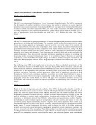
4904 JOURNAL OF CLIMATE VOLUME 23mixed layer temperature and ocean currents. The seasonalcycle of temperature along the equator is well simulatedby GODAS, and differences from the observed seasonalcycle are generally less than 0.58C (not shown). Zonalcurrent along the equator (18S–18N) is compared withOSCAR (Fig. 1). The OSCAR currents (Fig. 1a) arebased on an analysis of satellite altimeter and scatterometermeasurements, and the seasonal cycle is based onthe 1993–2007 analysis period (available online at http://www.oscar.noaa.gov/index.html). Compared to OSCARcurrents, GODAS has a westward bias in the far westernand eastern equatorial Pacific and an eastward bias in thecentral Pacific between 1808 and 1208W (Fig. 1c). Biasesin the western and central Pacific are likely associatedwith the assimilation of synthetic salinity, as these biasesare dramatically reduced in an experimental GODASassimilation run in which observed salinity from Argofloats is also assimilated (Behringer 2007).Next, GODAS and OSCAR currents are comparedwith the measurements at four TAO mooring locationsalong the equator in the western (1658E), central (1708W),and eastern (1408 and 1108W) Pacific. Figures 2a–h showthe annual cycles of zonal and meridional currents fromGODAS, OSCAR, and TAO observations, and Tables 1, 2show the comparison statistics between OSCAR andTAO and between GODAS and TAO. In Tables 1, 2,the mean bias was calculated as the mean differencebetween model and TAO data for the common periodof two datasets; rms errors (RMSEs) were calculatedwith the total currents; anomaly correlation coefficients(ACCs) and anomaly RMSEs (ARMSEs) were calculatedfrom currents for which the means have been removed.For zonal currents, OSCAR generally agrees withTAO better than GODAS does. The mean biases arerespectively 218, 13, 24, 22 cms 21 at 1658E, 1708W,1408W, and 1108W in OSCAR; and 224, 23, 13, and218 cm s 21 in GODAS (Table 1). The RMSEs are 19,14, 8, and 5 cm s 21 at 1658E, 1708W, 1408W, and 1108Win OSCAR; and 26, 26, 15, and 18 cm s 21 in GODAS(Table 1). Interestingly, both OSCAR and GODAS havereasonably high ACCs (0.93, 0.94, 0.95, and 0.98 inOSCAR; 0.76, 0.80, 0.96, and 0.98 in GODAS) withTAO observations. The anomalous RMSEs (5, 6, 7, and5cms 21 in OSCAR; 10, 11, 7, and 5 cm s 21 in GODAS)are much smaller than RMSEs that include the meanbiases. In summary, both GODAS and OSCAR havelarge mean biases in zonal currents in the western (1658E)and central (1708W) Pacific, and GODAS has muchlarger mean biases than OSCAR in the eastern (1408 and1108W) Pacific. Once the mean biases are removed, bothOSCAR and GODAS simulate TAO observations reasonablywell. It will be shown in section 5 that GODAS isquite adequate in simulating anomalous zonal advectiveFIG. 1. Zonal current (1993–2007) at 15-m depth along theequator (18S–18N) in (a) OSCAR, (b) GODAS, and (c) GODAS–OSCAR. Contour interval (C.I.) is 10 cm s 21 .heat flux in the central–eastern tropical Pacific associatedwith ENSO.For meridional currents, the OSCAR estimates aregenerally too weak and bear little resemblance to TAOobservations (Figs. 2e–h). In contrast, GODAS currentshave amplitudes comparable to those of observations.GODAS meridional currents are superior to OSCARmeridional currents in the western (1658E) and thecentral–eastern (1708 and 1408W) Pacific. The RMSEsare respectively 4, 8, 4, and 2 cm s 21 at 1658E, 1708W,1408W, and 1108W in OSCAR,; and 2, 4, 4, 3 cm s 21 inGODAS (Table 2). The ACCs are 0.59, 0.90, 0.56, and0.44 in GODAS but near zero in OSCAR, except in thefar eastern (1108W) Pacific.It is very interesting that, for zonal currents, OSCARis generally superior to GODAS in the central andeastern Pacific (1708, 1408, and 1108W) but both are poorin the western Pacific (1658E). An experimental GODASrun suggested that the large biases in GODAS zonal currentscan be significantly reduced when the Argo salinity

15 SEPTEMBER 2010 H U A N G E T A L . 4905FIG. 2. Zonal current (cm s 21 ) at (a) 1658E, (b) 1708W, (c) 1408W, and (d) 1108W and meridional current (cm s 21 ) at (e) 1658E, (f)1708W, (g) 1408W, and (h) 1108W. Currents are at 10-m depth for GODAS and TAO from current meters and at 15 m for OSCAR.Averaging periods for GODAS and TAO are 1986–2008, 2002–08, 1983–2008, and 1982–2004 at 1658E, 1708W, 1408W, and 1108W,respectively. The averaging period for OSCAR is 1993–2007. A 6-pentad running mean has been applied in the plots.is assimilated (Behringer 2007). For the meridional currents,GODAS is generally superior to OSCAR in thewestern (1658E) and central–eastern (1708 and 1408W)Pacific, but OSCAR is superior to GODAS in the easternPacific (1108W). However, the amplitude of GODASmeridional currents is more realistic than for OSCAR,which is too weak. The smaller RMSE in OSCAR thanin GODAS in the eastern Pacific is probably due to thesmaller amplitude in OSCAR.4. Methodology for analyzing the mixed layerheat budgeta. Mixed layer depthThe criterion to calculate mixed layer depth (MLD)is often defined differently based on requirements ofthe analysis (You 1995; Sprintall and Tomczak 1992).We select the criterion to be a density difference of0.125 kg m 23 between the surface and the bottom of themixed layer. The results of the heat budget analysis, however,are not sensitive to the choice of the criterion. In fact,similar results were obtained when the criterion waschosen to be a temperature difference of 0.5 K.The MLD of GODAS is calculated using the pentadfields of temperature and salinity. The seasonal cycle ofthe GODAS MLD is calculated based on the 1982–2004period and is compared with the MLD of WOD01, calculatedusing monthly climatological fields of temperatureand salinity in WOD01.The seasonal cycle of MLD along the equator (18S–18N) from WOD01 and GODAS, and their differences, isshown in Fig. 3. The WOD01 MLD is relatively shallow(deep) in the western and eastern (central) tropical Pacific(Fig. 3a). The shallow MLD in the eastern tropicalTABLE 1. Mean biases (MBIAS (positive toward east) (cm s 21 ), RMSE (cm s 21 ), anomalous correlation coefficient (ACC), andanomalous rms error (ARMSE), in which the means in each dataset were removed, of zonal currents between OSCAR and TAO andbetween GODAS and TAO.1658E 1708W 1408W 1108WOSCAR GODAS OSCAR GODAS OSCAR GODAS OSCAR GODASMBIAS 218 224 13 23 24 13 22 218RMSE 19 26 14 26 8 15 5 18ACC 0.93 0.76 0.94 0.80 0.95 0.96 0.98 0.98ARMSE 5 10 6 11 7 7 5 5

4906 JOURNAL OF CLIMATE VOLUME 23TABLE 2. As in Table 1 but for meridional currents: positive northward for MBIAS.1658E 1708W 1408W 1108WOSCAR GODAS OSCAR GODAS OSCAR GODAS OSCAR GODASMBIAS 4 1 7 4 3 4 22 22RMSE 4 2 8 4 4 4 2 3ACC 0.07 0.59 0.05 0.90 20.07 0.56 0.81 0.44ARMSE 2 1 3 1 2 2 1 2Pacific is associated with the shallow thermocline maintainedby easterly trade winds in the central tropical Pacific.The shallow MLD in the western tropical Pacificis associated with excess precipitation over evaporationthat forms a barrier layer (Sprintall and Tomczak 1992;Ando and McPhaden 1997). Compared to the WOD01,the MLD based on GODAS is about 20–30 m too deepin the west-central Pacific through the calendar yearand ;10–20 m too deep in the eastern Pacific duringboreal fall.b. Mixed layer temperature equationThe temperature equation for the mixed layer, describedby Stevenson and Niiler (1983), is expressed as(see details in appendix A)andT t5 F (1)F 5 Q u1 Q y1 Q w1 Q q1 Q zz, (2)where T t 5 ›T a /›t is the mixed layer temperature tendencyand F is the combined forcing of zonal advection(Q u ), meridional advection (Q y ), vertical entrainment(Q w ), adjusted surface heat flux (Q q 5 Q adj /rc p h), andvertical diffusion (Q zz 5 Q diff /rc p h); Q adj is the net surfaceheat flux plus heat flux correction minus the penetrativeshortwave radiation [see Eq. (A4)]. Weak horizontal diffusionwas ignored in our analysis.To understand the physical processes that control thetemperature variations in the mixed layer on differenttime scales, each variable associated with forcing F inEq. (2) is decomposed into low frequency variation($75 day) and high frequency transients (hereafter referredto as eddy). Therefore, Eq. (1) becomesT t5 Q L u 1 QL v 1 QL w 1 QL q 1 QL zz1 E, (3)where superscript L indicates the term calculated usinglow-pass filtered variables and E represents the combinedterms from high frequency eddies (see details inappendix B). Equation (3) is further decomposed intoclimatology (bar) and its anomaly (prime). The equationfor anomalous temperature is, omitting superscript L,T9 t5 Q9 u1 Q9 y1 Q9 q1 Q9 w1 Q9 zz1 E9. (4)Details about each term in Eq. (4) are described in appendixB. The climatological mean and annual cycle ofeach term in Eq. (3) will be discussed in sections 5b and5c. The anomalous heat budgets described by Eq. (4)will be used to construct a composite El Niño heat budget,and the characteristics of the anomalous heat budgetsfor a typical El Niño will be discussed in section 5d.A cutoff period of 75 days is chosen to separate seasonaland longer time scale variability from that associatedwith TIWs, which exhibit a typical period of 20–30days (Jochum and Murtugudde 2006). The annual climatologyof the heat budgets did not change much whendifferent cutoff periods between 30 and 90 days wereselected (as also indicated by KRC1998). This suggeststhat 60–90 day period oceanic Kelvin waves, forcedby the atmospheric Madden–Julian oscillation (MJO)and westerly wind bursts, do not make significant contributionsto the climatological heat budgets. However,the cumulative effects of a sequence of oceanic Kelvinwaves make a significant contribution to the anomalousheat budget on seasonal time scales and are believedto influence the onset and determination of El Niño (Seoand Xue 2005). In this paper, we will describe the heatbudget using an El Niño composite, which tends to smearout the contributions of oceanic Kelvin waves that may beof importance in the analysis of specific El Niño events.The topic of how a sequence of oceanic Kelvin wavescontributes to the anomalous heat budget on seasonaltime scales during a specific El Niño event will be exploredin a separate paper.c. Closure of the temperature equationTo test the procedures used for computing mixed layerbudgets, we first apply the proposed methodology to acontrol simulation (hereafter referred to as CNTRL) thatis identical to GODAS except no observations are assimilated.The pentad fields from CNTRL are used in the

15 SEPTEMBER 2010 H U A N G E T A L . 4907FIG. 3. Mixed layer depth (1982–2004) along the equator (18S–18N) in (a) WOD01, (b) GODAS, and (c) GODAS–WOD01: C.I. 510 m.calculation of all heat budget terms in Eq. (1). The pentadclimatology is calculated for 1982–2004, and pentadanomalies are obtained by removing the pentad climatologyfrom each heat budget term. The closure of theheat budgets is measured by the consistency between T tand F of Eq. (1). Figures 4a,b show the time evolutionof the T t and F for the annual cycle and interannualvariability in the Niño-3.4 region (58S–58N, 1208–1708W)during 1979–2007 in the CNTRL run. For both the annualcycle and the interannual variability, there is a closeresemblance in the tendency and forcing term. Temporalcorrelations between T t and F are above 0.95, andthe RMSEs are less than 0.098C month 21 . However, inthe annual cycle F is about 0.18C month 21 cooler than T tfrom June to December. The cold bias may be related tothe underestimation of the eddy warming in CNTRLduring summer/fall. In fact, the annual mean eddy warmingaveraged in the region 08–48N, 908–1408W in CNTRLis 0.58C month 21 , significantly weaker than 0.88C month 21derived in the model study by Richards et al. (2009). Theunderestimation of the eddy warming might be due to theuse of 5-day averaged fields and the 18 318 grid. The resultsnonetheless suggest that the temperature equationand its closure are approximately satisfied.Figures 4c,d show the seasonal cycle and interannualvariability of T t and F for GODAS. Data assimilationis expected to introduce sources and sinks of heat andgenerate inconsistency between the forcing fields andthe analyzed ocean states that will negatively impactthe closure of the mixed layer heat budget. However, themean seasonal cycle of T t and F follow each other closely,suggesting that the heat sources and sinks due to dataassimilation have only minor impact on the climatologicalheat budget. For the seasonal cycle, the ACCand RMSE between T t and F are 0.97 and 0.06, verysimilar to those for CNTRL. The influence of data assimilationon the heat budget is more evident in theevolution of T t and F anomalies, with an ACC (RMSE)of 0.70 (0.23), which is smaller (larger) than those forCNTRL. Note that a few factors contribute to the imbalancebetween T t and F, including sources and sinks ofheat due to data assimilation, and uncertainties in theparameterization of vertical entrainment and verticaldiffusion and the use of pentad fields and the 18318 grid.Therefore, we should not be surprised when T t ,andF areout of balance, as evident during the strong El Niño events(1982/83 and 1997/98; Fig. 4d). We will make a compositeheat budget for those weak-to-moderate El Niño eventswhere the closure is reasonably good and then analyze theheat budget during the strong El Niño events separatelywhere the closure is poor. We will also diagnose errors inthe heat budget through comparison with other observationaland model heat budget analyses.5. Analysis of the mixed layer heat budgeta. Surface heat fluxesThe net surface heat flux plays a critical role in forcingtemperature changes in the mixed layer in the equatorialPacific. The net surface heat flux forcings used in GODASis specified from the NCEP R2 reanalysis, and the climatologyof various components averaged in 1982–2004 isshown in Figs. 5a–d. Also shown are the climatologies ofpenetrative shortwave radiation (Fig. 5e), the surface heatflux correction (Fig. 5f) due to the SST relaxation inGODAS, and the adjusted net surface heat flux [Q adj ,Fig. 5g; see Eq. (A4)], which is the net surface heat fluxplus flux correction minus the penetrative radiation.Shortwave radiation exhibits a clear semiannual cyclealong the equatorial Pacific as the sun crosses the equatortwice a year (Fig. 5a). It has two maxima near the date linewith amplitude 240 W m 22 in October and 200 W m 22in April. The latent heat flux also has a semiannual cyclewith two maxima of 140 W m 22 in boreal winter and

15 SEPTEMBER 2010 H U A N G E T A L . 4909FIG. 5. Heat fluxes of the equatorial (18S–18N) Pacific Ocean: (a) downward solar radiation, (b) downwardlongwave radiation, (c) sensible heat, (d) latent heat, (e) penetrative solar radiation, (f) corrected heat flux inGODAS, (g) adjusted net heat flux, and (h) difference of net surface heat flux between GODAS and OAFlux: C.I. 5(a) 20, (b) 5, (c) 5, (d) 20, (e) 10, (f) 10, (g) 20, and (h) 20 W m 22 ; contours are shaded above (a) 220, (d) 120, (e) 30,(f) 20, and (g) 60 W m 22 and below (b) 250 and (h) 260 W m 22 .

4910 JOURNAL OF CLIMATE VOLUME 23(Fig. 5g). The analysis indicates that the longwave radiation,penetrative shortwave radiation, and heat fluxcorrections all make significant contributions to the closureof the heat budget, although their magnitudes arerelatively small compared with shortwave radiation andlatent heat fluxes.The latent and sensible heat fluxes shown in Fig. 5are similar to the OAFlux, and differences are generallyless than 10 W m 22 (not shown). Compared with the netsurface heat flux derived from the combination ofISCCP (shortwave and longwave) and OAFlux (latentand sensible) products, the net surface heat flux from R2is 40–60 W m 22 too low in the equatorial Pacific (Fig.5h), largely due to deficiencies in shortwave radiation.Shortwave radiation is 40–60 W m 22 too low in borealspring compared to ISCCP and WM99. Satellite datafrom ISCCP suggests that mean shortwave radiation isas large as 280 W m 22 in boreal fall and 260 W m 22 inearly boreal spring in the central equatorial Pacific (informationavailable online at http://oaflux.whoi.edu).To constrain the drift in surface temperature, GODASincludes a surface heat flux correction by relaxing modelSST to observed SST. The mean flux correction is about10–30 W m 22 (Fig. 5f). This correction partially compensatesfor biases in the net surface heat flux that, if notcorrected, would lead to a cooling of upper ocean temperatureduring the assimilation cycle. However, the correctionis not enough to compensate for all the deficienciesin the R2 net surface heat flux, which explains whyGODAS surface temperature is still about 0.28–0.48Ccooler than the observed SST (not shown).b. Annual-mean mixed layer heat budgetShown in Fig. 6 is the annual mean of the mixed layerheat budget calculated with the low-pass filtered GODASdata [Eq. (3)]. The mixed layer is heated on averageby the adjusted surface heat flux (Q q ) at a rate of 0.2–0.58C month 21 in the central and western Pacific and1–38C month 21 in the eastern tropical Pacific (Fig. 6d).The heating is largely balanced by the cooling frommeridional advection (Q y , Fig. 6b), vertical entrainment(Q w , Fig. 6c), and vertical diffusion(Q zz , Fig. 6e). Themaximum cooling by meridional advection is centered offthe equator with a magnitude of 18C month 21 near 28Nand 0.58C month 21 near 38S intheeasterntropicalPacific.The cooling from Q w is 0.28Cmonth 21 in the centraltropical Pacific and 18C month 21 in the far eastern tropicalPacific. The cooling is larger from vertical diffusionthan from vertical entrainment, and the meridional extensionis also broader because upwelling is mainly constrainedwithin a narrow equatorial band. The annualmean zonal advection (Q u , Fig. 6a) contributes to a weakcooling (0.28C month 21 ) across much of the tropicalPacific. TIW heating (Fig. 6f) is approximately 0.28Cmonth 21 in the eastern tropical Pacific east of 1508W,and is weaker than in CNTRL (0.58C month 21 ), ZH08(0.58C month 21 ), Richards et al. (2009; 0.88C month 21 ),and Jochum and Murtugudde (2006; 28C month 21 ).c. Seasonal cycle of the mixed layer heat budget1) SEASONAL CYCLE IN GODASThe seasonal cycle of the mixed layer heat budget inthe equatorial Pacific (0.58N, which is selected for thepurpose of comparison in the following subsection) isdiscussed next. The mixed layer temperature tendencyhas a strong seasonal cycle in the equatorial easternPacific (Fig. 7e). The positive tendency in early borealspring is largely due to excess heating by the adjusted netsurface heat flux (Q q ) (Fig. 7d) over cooling by verticalentrainment and diffusion (Q w 1 Q zz ) (Fig. 7c). Incontrast, the negative tendency during late boreal springto summer is due to cooling by Q w 1 Q zz and Q y dominatingover heating by Q q .The heating by Q q is dominated by a semiannual cycle(Fig. 7d). It is the largest in the equatorial eastern Pacific,with a primary maximum in boreal spring (48Cmonth 21 )and a secondary maximum in boreal fall (28C month 21 ).The seminannual variation of the heating by Q q is criticallycontrolled by cloudiness and mixed layer depth, aswas pointed out by KRC98. The magnitude of Q q is muchweaker (0.58C month 21 ) in the central and westerntropical Pacific than in the east, because the MLD isrelatively deep in the west. Heating in the west–centraltropical Pacific is dominated by the semiannual signalin shortwave radiation (Fig. 5a), which largely governsthe temperature tendency (Fig. 7e).Cooling by Q w 1 Q zz remains confined to the centraland eastern tropical Pacific, where the MLD is shallowand the vertical temperature gradient is the largest. Thecooling has a primary maximum in boreal spring and asecondary maximum in boreal summer.The contribution of Q u is the largest east of 1308W(Fig. 7a) and is dominated by the seasonal cycle: coolingfrom February to June and a heating from July to January.This cooling exhibits westward propagation, with coolingin the central and eastern Pacific in the fall (Fig. 7a).The cooling from Q y is the largest from May to Decemberwhen northerly currents are the strongest (Fig. 2h).The seasonal cycle of TIW heating (Fig. 7f) is about0.58C month 21 east of 1308W from June to December.2) COMPARISON WITH OTHER MODELSIMULATIONSThe seasonal variation of Q q in the equatorial Pacificis similar to that in WM99. The seasonal variation of

15 SEPTEMBER 2010 H U A N G E T A L . 4911FIG. 6. Averaged (1982–2004) and low-pass filtered temperature budgets by (a) zonal advection, (b) meridionaladvection, (c) entrainment, (d) adjusted surface heating, and (e) vertical diffusion; (f) eddy: contours are 0, 60.2,60.5, 61, 61.5, 62, and 638C month 21 .Q w 1 Q zz is close to that of ZH08. The pattern of TIWheating is almost the same as in ZH08.A potential bias in GODAS is the zonal advectivecooling in the eastern tropical Pacific in boreal spring(Fig. 7a), which is inconsistent with results reported inearlier studies. KRC98 and ZH08 suggested that Q uis weakly positive east of 1208W during boreal springlargely owing to the spring reversal of the South EquatorialCurrent (SEC). The erroneous cooling by Q u inGODAS is associated with errors in the surface zonal

4912 JOURNAL OF CLIMATE VOLUME 23FIG. 7. Low-pass filtered temperature budgets at 0.58N by (a) zonal advection, (b) meridional advection, (c) entrainmentand vertical diffusion, and (d) adjusted surface heating: (e) unfiltered temperature tendency and (f) eddy.Contours are 0, 60.5, 61, 61.5, 62, 63, 64, and 658C month 21 .currents in GODAS for which the spring reversal of SECdoes not extend as far eastward as in OSCAR (Fig. 1).The negative Q u in GODAS is generated by the westwardsurface zonal currents east of 1058W (Fig. 1b). Comparedwith the analysis of ZH08, the cooling in boreal fall andwinter is confined too narrowly in the eastern Pacific andis related to the eastward biases in GODAS surfacezonal currents in the region (Figs. 1c, 2a–d).Cooling from Q y in the eastern Pacific appears toostrong in GODAS (0.58–38C, Fig. 7b) when compared

15 SEPTEMBER 2010 H U A N G E T A L . 4913with that in ZH08 (0.58C). Considering that GODASmean meridional currents do not agree well with observationsin the eastern Pacific at 1108W (Table2)andGODAS mean temperature has cold biases in the region(not shown), the Q y climatology is likely problematic inthe eastern Pacific. In addition, the TIW heating inGODAS (Fig. 7f) is only half of ZH08 (18C month 21 )andCNTRL (18C month 21 ) and extends westward to only1258W compared to 1508W in ZH08 and CNTRL.3) COMPARISON WITH OBSERVATIONALANALYSESWe use the observational analysis of WM99 to furthervalidate the heat budgets of the mixed layer in GODAS.WM99 used observed winds, temperature, and oceancurrents from the TAO moorings at four locations alongthe equator in the western (1658E), central (1708W), andeastern (1408 and 1108W) Pacific. Changes in heat storage,horizontal heat advection, and heat fluxes at thesurface in WM99 were estimated directly from data. Intheir estimates, vertical heat flux out of the base of themixed layer was calculated as residual and surface heatfluxes were from COADS. The heat budgets in GODASare calculated using unfiltered (total) data to facilitatecomparison with WM99.The temperature tendencies in the mixed layer ofGODAS at the four TAO sites are shown in Fig. 8a.According to WM99, the temperature at 1108W warmsfrom September to March and then cools from April toAugust. This seasonal variation is replicated by GODASexcept the strong cooling tendency in June is underestimatedand the weak warming tendency in Novemberis missing. Because of the westward propagation of positiveclimatological SSTs, the peak warming tendency at1108W, 1408W, 1708W, and 1658W subsequently progresseswestward from February to April. This westwardpropagation of climatological SST is well simulated byGODAS. The secondary maximum warming at 1658E inboreal fall indicates a semiannual cycle in the westerntropical Pacific (Yuan 2005).Zonal advection, Q u , generally cools the eastern(1108W) tropical Pacific during August to February whenthe SEC is westward and warms it during the spring reversalof the SEC (Fig. 8b). The warming at 1108W inMarch–June (Fig. 6b in WM99) is simulated as coolingin GODAS (Fig. 8b), mainly because GODAS underestimatesthe spring reversal of the SEC in the fareastern Pacific. The cooling at 1108W in boreal fall isseriously overestimated by GODAS owing to westwardbiases in the surface zonal currents (Figs. 1c and 2d).Relative to 1108W, Q u at 1408 and 1708W is much bettersimulated by GODAS, in good agreement with the observationalanalysis of WM99. Zonal advection at 1658Ecools throughout the year and is largely consistent withWM99.Meridional advection Q y , at 1108 and 1408W leadsto warming along the equator with maximum amplitudein boreal summer and fall due to active TIWs (WM99;Chen et al. 1994; KRC98). The Q y reaches a minimumduring early boreal spring when TIWs are inactive(WM99). In GODAS, warming by Q y at 1108 and 1408W(Fig. 8c) is much weaker (0.28–0.58C month 21 ) than inWM99 (0.58–28C month 21 ) and has a secondary maximumwarming during boreal spring (Fig. 8c). The weakwarming in Q y at 1108 and 1408W is partly due to biasesin the mean meridional currents (Figs. 2g,h) and partlyto weak TIWs. Biases in the low-frequency meridionalcurrents may be associated with biases in wind forcingand biases that result from assimilating synthetic salinityrather than the observed salinity (Huang et al. 2008).Heating by Q q (Fig. 8d) is the largest in the easternPacific owing to a shallow MLD (Fig. 1b) and is dominatedby a semiannual cycle at all four sites. The Q q inGODAS agrees well with that in WM99. One noticeabledisagreement is that the second maximum at 1108Wduring boreal fall is about twice as large as in WM99. Thedifferences may result from different methods in calculatingQ q , although the adjusted net heat flux (Fig. 5g)and MLD (Fig. 1b) in GODAS agrees very well withthose of WM99. The climatology of Q q in GODAS iscalculated with the pentad Q q in the period 1982–2004and therefore retains the nonlinear relationship betweenthe adjusted net heat flux and MLD [Eq. (A9)]. Incontrast, the climatology of Q q in WM99 is based on theclimatology of the adjusted net heat flux divided by theclimatology of MLD. It should also be noted that there isconsiderable uncertainty in the mean seasonal cycle ofnet heat flux itself (Wang and McPhaden 2001b).The combined cooling by Q w 1 Q zz (Fig. 8e) is thelargest in the eastern Pacific due to the shallow MLD andstrong upwelling in the region. The Q w 1 Q zz generallyagrees well with those in WM99. However, cooling at1108W in April–August is significantly underestimated inGODAS. The cooling at 1408WisalsoweakerinGODASthan in WM99. The weaker cooling by entrainment andvertical diffusion in GODAS may be associated withbiases in zonal wind stress in R2, which is too weak whencompared with Quick Scatterometer (QuikSCAT) observationsand other products (Josey et al. 2002). The treatmentof the vertical entrainment and vertical diffusion asa residual in WM99 may also contribute to the differencebetween GODAS and WM99.4) DISCUSSIONMitchell and Wallace (1992) suggested that the seasonalcycle of SST and its westward propagation are

4914 JOURNAL OF CLIMATE VOLUME 23FIG. 8. Unfiltered temperature budgets of the equatorial Pacific Ocean at 1108W, 1408W, 1708W, and 1658E: (a)temperature tendency, (b) zonal advection, (c) meridional advection, (d) adjusted heat flux, and (e) entrainment andvertical diffusion: (8C month 21 ). A 6-pentad running mean has been applied in the plots.driven by a weakened vertical mixing from December toMarch due to a weakened meridional wind. Xie (1994)further proposed that the weakened vertical mixinglargely result from the coupling of SST, meridional wind,and evaporation. KRC98 suggested that both net heatfluxes and vertical mixing contributed to the warmingtendency from late winter to early spring. They alsopointed out that the solar radiation in spring is largerthan that in fall owing to a minimum in cloud cover inspring. WM99 suggested that net surface heat fluxes andresidual subsurface fluxes, equivalent to the combinationof vertical entrainment and vertical diffusion, are the twodominant terms and tend to cancel out each other duringspring. They emphasized a large warming due to TIWsduring fall/winter and a correlation between the meanannual cycle of residual subsurface fluxes and zonal winds,

15 SEPTEMBER 2010 H U A N G E T A L . 4915which implied that the subsurface fluxes are the weakestduring spring when zonal winds are the weakest. Vialardet al. (2001) suggested the annual cycle of SST in theNiño-3 region is largely controlled by net surface heatfluxes.Compared to aforementioned results, the annual cycleheat budget in GODAS has several shortcomings. First,the TIW warming in boreal fall is severely underestimatedin GODAS (Fig. 7f). Second, the low-frequency meridionaladvection, Q y , is too strong in boreal summer/fall(Fig. 7b). The biases in Q y are probably due to too strongcross-equatorial winds in the NCEP reanalysis duringsummer/fall (not shown) that are used to force the MOM3model. Third, the Q w 1 Q zz in boreal summer/fall appearstoo weak compared to that in WM99, KRC98, andVialard et al. (2001) (not shown).Despite these shortcomings, GODAS analysis showsthat a positive temperature tendency in the tropicaleastern Pacific from December to March is associatedwith the strengthening of heating by the adjusted heatflux, consistent with WM99, KRC98, and Vialard et al.(2001). This term dominates over the intensification incooling by vertical mixing, both of which are associatedwith a shoaling mixed layer depth from December toMarch (Fig. 3b). The shoaling mixed layer depth is alsoclosely related to surface heat fluxes and surface winds.Therefore, a weakening surface winds, strengthening netsurface heat fluxes, and shoaling mixed layer depth allcontribute to the warming tendency of SST from Decemberto March.d. El Niño composite of mixed layer heat budgetIn the previous section, the annual mean and the seasonalcycle of the mixed layer heat budget based onGODAS pentad output were discussed. Another importantfeature of coupled variability in the equatorial tropicalPacific is ENSO. The ENSO phenomenon (Philander1990) is the most prominent interannual climate signal,so the ability of GODAS to capture the variability of themixed layer heat budget during the ENSO cycle is assessednext.1) EL NIÑO COMPOSITEAs defined by the NOAA official ENSO index, theOceanic Niño Index (ONI), there were eight warm episodesfrom 1979 to the present that occurred in 1982–83,1986–88, 1991–92, 1994–95, 1997–98, 2002–03, 2004–05,and 2006–07. Many studies have shown that ENSO episodesare phase locked to the seasonal cycle (Changet al. 1995; Tziperman et al. 1998; Galanti and Tziperman2000; McPhaden and Zhang 2009). The onset of ENSOevents generally occurs early in the year and becomesmature late in the year or early in the next year (Rasmussonand Carpenter 1982) with the exception of the 1986–88event, whose onset and mature phases were differentfrom others.An El Niño composite is constructed using five weakto-moderateevents (1991–/92, 1994–95, 2002–03, 2004–05,and 2006–07). The 1986–87 event was excluded becauseof its unique onset and decay phases. The 1982–83 and1997–98 events are strong events in which nonlinearterms are likely very different from those during weakto-moderateevents (Jin et al. 2003). In addition, theanalysis suggests that the closure of the heat budgetduring the two events is not as good as during otherEl Niño events. We therefore compare the heat budgetof the two events with that discussed in literature separatelyand assess the feasibility of GODAS in simulatingthe two strongest events in the past 30 years.2) HEAT BUDGET FOR THE COMPOSITE EL NIÑOShown in Fig. 9 are the mixed layer heat budgets forthe El Niño composite averaged between 18S and18Nin GODAS. The composite El NiñostartsinJanuaryofan El Niño (year 0) and ends in a following La Niña(year 11, Fig. 9h). The analysis indicates that heatingby entrainment and vertical diffusion (Q w 1 Q zz ,Fig.9c),meridional advection (Q y , Fig. 9b), and zonal advevction(Q u , Fig. 9a) contribute to El Niño developmentduring year 0: The heating by Q w 1 Q zz and Q y is thestrongest east of 1408W; and the heating by Q u is distributedover most of the tropical Pacific between 1608Eand 1108W. The adjusted surface heat flkux (Q q ) ismostly opposite to the composite SST anomalies (Fig. 9h)and strongly acts to damp El Niño in the eastern tropicalPacific in year 0 and early year 11. TIW heating (Fig. 9e)also acts weakly to damp El Niño development.El NiñotransitstoLaNiña around April of year 11. Amoderate cooling (20.58 to approximately 218Cmonth 21 )by Q u and Q q plays a critical role during the period priorto the transition, while both Q w 1 Q zz and Q y still contributeto a heating in the central-eastern Pacific. Therefore,zonal advection leads the transition from El Niñoto La Niña.After the decay of El Niño, cooling by Q w 1 Q zz , Q y ,and Q u becomes strong, leading to La Niña developmentduring the summer/fall of year 11. Strong heating by Q qacts again to damp La Niña development later in year 11.The balance between temperature tendency (Fig. 9f)and forcing (Fig. 9g) appears to be good in the centraleasterntropical Pacific, but it is worse in the far easterntropical Pacific largely due to biases in zonal currents(Fig. 1c) and the underestimation of TIW heating (Fig. 6f),which is anomalously weak (strong) during El Niño (LaNiña) events (Yu and Liu 2003). The underestimation ofTIW heating in GODAS largely resulted from applying

4916 JOURNAL OF CLIMATE VOLUME 23FIG. 9. Low-pass filtered temperature budgets of the El Niño composite between 18S and 18N by (a) zonal advection,(b) meridional advection, (c) entrainment and vertical diffusion, and (d) adjusted surface heat. (e) Eddybetween unfiltered and low-pass-filtered budgets; (f) unfiltered temperature tendency; (g) unfiltered forcing inEq. (2), and (h) unfiltered temperature. Contours are 0, 60.2, 60.5, 61, 61.5, and 62. Units are 8C month 21 in(a)–(g) and 8C in (h). A 6-pentad running mean has been applied in the plots.

15 SEPTEMBER 2010 H U A N G E T A L . 4917FIG. 10. Temperature budget anomalies of the El Niño composite in the Niño-3.4 region (58S–58N, 1208–1708W).(a) Unfiltered temperature budgets (8C month 21 ). Decomposition of low-pass filtered (b) zonal advection, (c) meridionaladvection, and (d) entrainment and vertical diffusion. The unfiltered budgets in (a) are replotted in (b)–(d).Temperature anomalies are plotted in the scale of the right axis. Decomposition of climatology and associatedanomaly are noted as bar and prime, for example, UbarT9 5u T9 xin (b). The ‘‘eddy’’ in (b)–(d) represents thedifference between the unfiltered budget anomaly in (a) and low-pass filtered budget anomaly.a 4-week data assimilation window that smoothes outvariations shorter than 30 days. The TIW signal is furtherweakened by using pentad outputs on the 18 318 grid,which is available for the analysis.The roles of different oceanic processes and surfaceheat fluxes in the El Niño composite in GODAS is furtherdiscussed for the Niño-3.4 SST index region (58S–58N, 1208–1708W). Figure 10a shows the spatial averageof each flux term in the Niño-3.4 region. Lee et al. (2004)suggested that spatially integrated local temperature advectioncan be dominated by internal processes such asTIW that redistribute heat within the domain and theyrecommended a new boundary flux approach to analyzethe mixed layer heat budget. Kim et al. (2007) furthershowed that the spatially integrated zonal advection tendencyin the Niño-3 region derived from ECCO analysis isanticorrelated with the change of SST during the 1997–99El Niño–La Niña cycle, which disagrees with the commonunderstanding about the role of large-scale advection ofwarm pool water during El Niño. Ultimately, the two approachesmust be consistent with one another when allterms in the heat balance are accounted for and properlyinterpreted, so our preference is to perform the analysisbased on the more conventional local balance approach.In this analysis the advective temperature terms arefurther decomposed into various components describedin Eqs. (B5)–(B8). It is seen in Fig. 10a that the positivetemperature tendency during the spring of year 0 is dueto heating from Q w 1 Q zz , Q y , and Q u . The temperaturetendency changes sign from positive to negative at theend of year 0, which coincides with a rapid transition ofQ u from heating to cooling. It is interesting that Qv doesnot have a transition until 4–5 months later. This suggeststhat cooling from Q u and Q q plays a dominant roleduring the decay phase of El Niño and transition to thefollowing La Niña, consistent with ENSO recharge–discharge theory (Jin 1997). During the summer and fallof year 11, cooling from Q y and Q u all contribute to thetransition from El Niño to La Niña as well as the developmentof La Niña. However, Q w 1 Q zz does not appearto contribute to the development of La Niña in weak-tomoderateevents, which is not the case for strong eventssuch as in 1997–98 and 1982–83, which will be discussedlater.

4918 JOURNAL OF CLIMATE VOLUME 23The decomposition of Q u in Fig. 10b shows that theheating by Q u during El Niño development in year 0 isdominated by u9T x(subscripts x, y, and z representa partial derivative, hereafter), and the cooling by Q uduring La Niña development in year 11 is also associatedwith u9T x. This suggests an important role ofthe zonal advection of climatological temperature byanomalous zonal currents in El Niño and La Niña development.Note that uT9 xacts to weakly dampEl Niño and TIW acts to weakly damp both El Niño andLa Niña. For meridional advection, the heating (cooling)by Q y (Fig. 10c) during the development of El Niñoin year 0 (La Niña in year 11) in GODAS results fromboth yT9 yand y9T ythat have comparable amplitude.The decomposition of Q w 1 Q zz in Fig. 10d shows thatboth wT9 zand w9T zcontribute to the development ofEl Niño and their amplitudes are comparable. Duringthe onset phase of El Niño, both w9T zand wT9 zareimportant, suggesting that the role of upwelling anomalies( w9T z) is as important as subsurface temperatureanomalies ( wT9 z)whenElNiño is beginning to develop.During the decay phase of El Niño and developmentphase of La Niña, all components in Q w 1 Q zz act asa weak warming (Fig. 10d), which is quite different fromthose during the strong events of 1997–98 and 1982–83.3) DISCUSSIONBase on GODAS, the onset phase of El Niño can beattributed to the heating by Q u , Q y , and Q w 1 Q zz , whichis largely consistent with observational analysis in Wangand McPhaden (2000). Since Q u is dominated by u9T xin GODAS (Fig. 10b), anomalous zonal currents actingon the large climatological SST gradient near the easternedge of the warm pool plays a critical role during theonset phase of El Niño, a feature also noted in previousobservational studies (Frankignoul et al. 1996; Picaut et al.1996; Wang and McPhaden 2000). The results based ona coupled model simulation also suggested the importanceof Qu in El Niño development (Zhang et al. 2007).Meridional advection (Q y ) contributes to the developmentof El Niño east of 1408W in GODAS (Fig. 9b).The decomposition of Q y indicates that both yT9 yandy9T ymake important contributions to El Niño developmentin GODAS, while coupled model simulation(Zhang et al. 2007) suggested that y9T yis not as importantas yT9 y. Wang and McPhaden argued that Q y isa damping since TIW dominates this term at the equatorand generally acts as a damping to SST, as indicatedin model simulations (Yu and Liu 2003; ZH08; An 2008).This is also true in our analysis of GODAS in the equatorialPacific (Figs. 10b,c), but the TIW term is underestimatedby GODAS (Fig. 8c).The decomposition of Q w 1 Q zz (Fig. 10d) showsthat both wT9 zand w9T zcontribute to the onset phaseof El Niño in GODAS. This suggests that both w9 andsubsurface temperature anomalies (T9) are key variablesto determine El Niño onset, consistent with other observationalstudies (Wang and McPhaden 2000, 2001a;Zhang and McPhaden 2006, 2008). The separation ofQ w 1 Q zz (not shown) indicates that Q zz plays an importantrole in the heat budget of the El Niño compositein GODAS. The observational analyses of 1987–88(Hayes et al. 1991) and 1991–93 (Kessler and McPhaden1995) El Niño events, model analysis of the 1997–98 event(Kim et al. 2007), and a coupled model simulation (Zhanget al. 2007) all suggested the important role of Q zz .During the decay phase of El Niño, both Q u and Q yplay a leading role in GODAS. In fact, Q u leads Q y by4–5 months (Fig. 10a). Zonal advection (Q u ) is dominatedby u9T x, which suggests that anomalous zonal currents area precursor for the transition from El Niño toLaNiña.These results are very consistent with previous studiesbased on observations (Wang and McPhaden 2000, 2001a;Vialard et al. 2001) and with coupled model simulations(An and Jin 2001; Zhang et al. 2007). Observationalstudies of Wang and McPhaden (2000, 2001a) suggestedthat Q q acts as a damping to El Niño because of the outof-phaserelationship between SST and Q q . This dampingis particularly important during the decay phase ofEl Niño (Figs. 10a and 9d).The Q q anomaly is largely due to latent heat flux (Q lh ,Fig. 11a) and its dependence on anomalies of SST andother near-surface atmospheric variables. Shortwave radiation(Q short ) contributes secondarily to cooling duringthe peak phase of El Niño. Penetrative solar radiation(Q pen ) contributes to heating (cooling) when mixed layerdepth is anomalously deep (shallow). Longwave radiationand sensible heat flux (Q long 1 Q sh ) are generally weak.The flux correction (Q corr ) resulting from relaxation toobserved SST is relatively large during the developmentphase of El Niño and La Niña, indicating biases in surfaceheat fluxes and errors in the model physics.For the two strong events of 1997–98 and 1982–83, themixed layer heat budget closure is generally poor (Fig.2d). We pointed out earlier that the imbalance betweenF and T t may result from multiple factors, includingsources and sinks of heat due to data assimilation, andestimation of vertical diffusion. It should also be notedthat the evolution of mixed layer heat budget duringstrong El Niño events may differ significantly from thatfor weak-to-moderate El Niño events.Next, we assess if it is feasible for GODAS to simulatethe mixed layer heat budget of the 1997–98 and 1982–83events, which are the biggest of the past 30 years. Figure12a shows the GODAS budget at 08, 1108W from 1997 to

15 SEPTEMBER 2010 H U A N G E T A L . 4919FIG. 11. (a) Components of surface heat flux anomalies (left axis)and MLD anomaly (right axis) of the El Niño composite in theNiño-3.4 region (58S –58N, 1208–1708W). Fluxes are positive downwardexcept for Q pen , which is positive upward. (b) Mixed layer heatbudget closure (left axis) and mixed layer temperature anomaly(right axis) in the Niño-3.4 region.1998. It is clear that the development of the El Niño in1997 is largely associated with the anomalous heatingby subsurface Q w 1 Q zz and zonal advection Q u . Thetransition from El Niño to La Niña results from theanomalous cooling by Q u and net Q q . The developmentof La Niña in 1998 is largely associated with the anomalouscooling by Q w 1 Q zz and Q u . These features arelargely consistent with the heat budget composite forweak-to-moderate events (Fig. 10a). Differences arethat anomalous cooling by Q w 1 Q zz played the dominantrole in the development of La Niña in 1998, whileQ w 1 Q zz acts as a weak damping in the composite.Meridional advection Q y did not contribute much tothe development of El Niño and acted as a damping tothe development of the La Niña in 1998. However, Q ycontributed significantly to the development of thecomposite El Niño and La Niña (Fig. 10a). The roles ofQ w 1 Q zz and Q q in our analysis are consistent with theobservational analysis of Wang and McPhaden (2001a,their Fig. 6). However, the magnitude of Q w 1 Q zzand Q q appears to be underestimated in our analysis.Some differences were also found in Q u and Q y betweenGODAS and observations. Zonal advection (Q u ) contributedto the development of El Niño in GODAS in1997, which is consistent with observations. However, itcontributed significantly to the development of La Niñain GODAS in 1998 instead, being a weak damping asin the observations. Further analysis showed that theanomalous cooling by Q u in GODAS in 1998 is largelyassociated with u9T x(Fig. 12b) because of westwardbiases in zonal current anomalies (Fig. 12d). Meridionaladvection (Q y ) contributed moderately to the developmentof El Niño in 1997 in the observation, but it wasnegligible in GODAS (Figs. 12a,c). TIW acts as a weakdamping to the El Niño in 1997 and La Niñain1998(Figs.12b,c). Differences at the other three TAO mooring sites(1408, 1708W; and 1658E) are also large (not shown).For the 1982–83 event (Fig. 13a), anomalous heatingand cooling by Q w 1 Q zz played a dominant role in thedevelopments of El Niño and La Niña in GODAS,which is very consistent with the observational analysisof Wang and McPhaden (2000, their Fig. 5), although themagnitude of these terms was weaker in GODAS thanin observations. Anomalous cooling by Q q damped theEl Niño in 1982, consistent with observations. Anomalousheating by Q u contributed to the development ofEl Niño in GODAS in 1982, which is also consistent withobservations; however, it became too strong in 1983compared with the observations. This is largely due tothe nonlinear heating (mainly 2u9T9 x , Fig. 13b) thatappears to be associated with strong westward biasesof zonal current in GODAS (Fig. 13d). In observations,anomalous cooling by Q y damped the development ofthe El Niño in 1982 but contributed to the developmentof the La Niña in 1983. However, in GODAS Q y is veryweak in 1982 and is a moderate damping to the developmentof the La Niña in 1983 because of heatingfrom y9T yand the nonlinear term (Fig. 13c). The TIWacts as a weak damping to the El Niño in 1982 and LaNiña in 1983 (Figs. 13b,c).The above results suggest that GODAS simulates Q qand Q w 1 Q zz reasonably well, but contain large biasesin Q u and Q y , most of which are due to biases in surfacecurrents. It is found that surface current analysis nearthe equator can be significantly improved when observedsalinity is assimilated into GODAS and the balance betweendensity and current is properly maintained in theanalysis cycle (Behringer 2007). Therefore, we hope thatbiases in Q u and Q y will be significantly reduced in thenext version of GODAS in which the Argo salinity will beassimilated.

4920 JOURNAL OF CLIMATE VOLUME 23FIG. 12. Temperature budget anomalies at 08, 1108W from 1997 to 1998: (a) unfiltered temperaturebudget (8C) at 08N, 1108W; decomposition of low-pass filtered (b) zonal and (c) meridionaladvection; and (d) zonal current of TAO and GODAS for the 1997–98 El Niño event at08N, 1108W and 35-m depth. A 5-month running mean and a 3-month running mean have beenapplied in (a)–(c) and a 3-month running mean in (d).6. Summary and discussionThe focus of this paper is to assess the adequacy ofGODAS pentad data to provide a consistent picture of themixed layer heat budget in the tropical Pacific from 1979 topresent. We have demonstrated that the mean mixed layerdepth was reasonably well simulated by GODAS eastof the date line but was about 10–20 m too deep in thewestern Pacific, probably because the water in the westernPacific warm pool was too salty (Behringer 2007).The climatological mean and seasonal cycle of mixedlayer heat budgets derived from GODAS agree reasonablywell with previous observational (WM99) andmodel-based estimates (KRC98; Vialard et al. 2001).However, significant differences and biases were noticed.The net surface heat fluxes into the ocean derived fromthe NCEP R2 and used to force GODAS are about 40–60 W m 22 too low in the eastern equatorial Pacific duringboreal spring (Fig. 5h). Large biases were also foundin GODAS zonal and meridional currents (Tables 1, 2),

15 SEPTEMBER 2010 H U A N G E T A L . 4921FIG. 13. As in Fig. 12 but for the 1982–83 El Niño event.which contributed to biases in the annual cycle of zonaland meridional advective heat fluxes, Q u and Q y (Figs.7a,b). However, the interannual variability of the mixedlayer heat budget has been simulated reasonably wellby GODAS. This is demonstrated using the compositeof anomalous heat budget for five weak-to-moderateEl Niño events (Figs. 9, 10). The results, therefore, suggestthat GODAS provides a reasonable estimate ofboth the seasonal cycle and interannual variability in themixed layer heat budget. We conclude, therefore, thatit is a useful tool for real-time monitoring of mixed layervariability and for further understanding coupled ocean–atmospheric interactions.The mixed layer heat budget analysis tool derivedfrom GODAS can also be derived from other operationalocean reanalyses (ORAs) routinely produced byoperational centers (Balmaseda et al. 2008; Oke et al.2005; Alves and Robert 2005). The effort of derivingmultimodel heat budget analyses would likely enhanceour confidence in the feasibility of ORAs for monitoringand understanding tropical Pacific SST variability. Monitoringthe differences among multimodel analyses willalso help us identify common biases and deficiencies inORAs and the requirements those ORAs impose on theocean observing system for operational data streams(Xue et al. 2010). As the ORAs also provide initial

4922 JOURNAL OF CLIMATE VOLUME 23conditions for seasonal climate predictions, the mixedlayer heat budget analysis presented here can also beapplied to understand the evolution of the SST anomaliesin the forecast, as well as to understand the initialadjustments (sometimes referred to as initial shock) anddevelopment of coupled model biases.Acknowledgments. We thank Dr. Kelvin Richards,Dr. Shangping Xie, and an anonymous reviewer for theircritical and constructive comments, which helped us improvethe manuscript significantly. We also want to thankDr. David Behringer, who provided us detailed informationabout the GODAS ocean analysis and for helpfuldiscussions on our results. This work was partially supportedby the Climate Test Bed of NOAA and also byNOAA’s Climate Program Office.APPENDIX ATemperature EquationThe temperature equation for the mixed layer, describedby Stevenson and Niiler (1983), is adopted here:h ›T a5 hv›t a $T aw e3 (T aT h)ð 0$ ( ^v ^Tdz) 1 (Q OQ pen1 Q corrh1 Q diff)/rc p, (A1)where h is MLD; T and v are temperature and horizontalcurrents; subscript a represents quantities that are verticallyaveraged between the surface and h; ^v and ^T in thethird term on the right-hand side are deviations fromtheir vertically averaged quantities, and their contributionto the heat budgets is generally very small in the mixedlayer (ZH08) and neglected in our discussions; w e is theentrainment velocity across the bottom of the mixedlayer, calculated byw e5 ›h›t 1 v h $h 1 w h , (A2)where w 2h is the vertical velocity at the bottom ofthe mixed layer. The last four terms in Eq. (A1) arevarious heat flux terms: Q O is the net downward surfaceheat fluxes, composed of shortwave (Q short ) and longwave(Q long ) radiation, latent (Q lh ) and sensible (Q sh )heat fluxes; Q pen is the shortwave radiation transmittedthrough the bottom of MLD and is parameterized(Pacanowski and Griffies 1999) asQ pen5 Q short(0.58e h/0.35 1 0.42e h/23 ).(A3)Here Q corr represents a heat flux correction introduced bya relaxation of model SST to observed SST in GODAS.Following WM99, we define the adjusted net surface heatflux asQ adj5 Q OQ pen1 Q corr. (A4)The last term on the rhs of Eq. (A1), Q diff , is the diffusiveheat flux at the bottom of the mixed layer and is parameterized(Hayes et al. 1991) asQ diff5 rc pK z›T›z(A5)in which r and c p are density and heat capacity of seawater;K z5 K c1n1 1 bRi(A6)in which K c 5 13 10 25 m 2 s 21 , b 5 5, and Ri is theRichardson number defined asRi 5 ag ›T›z 3 [(›u/›z)2 1 (›y/›z) 2 ] 1 , (A7)where a 5 8.75 3 10 26 (T 1 9)8C 21 and g 5 9.8 m s 22 ;a minimum Ri is set to 20.1 to ensure valid diagnosis;and n in Eq. (A6) is parameterized asn 5 n c1 n 03 (1 1 bRi) 2 ,(A8)where n c 5 1 3 10 24 and n 0 5 3.5 3 10 23 m 2 s 21 .Weshould point out that the diffusion parameterizationused in our analysis in (A5)–(A8) is much simpler thanoriginally implemented in GODAS [the K-profile parameterization(KPP) vertical mixing scheme, Largeet al. (1994)], which may result in the imbalance of heatbudgets. Horizontal diffusion has been neglected owingto its small magnitude.We also note that vertical entrainment and diffusionare sometimes treated as a residual to keep the closureof mixed layer heat budgets (WM99). They were oftencombined and parameterized to be proportional to verticaldifferences between the temperatures in and below themixed layer. One common parameterization is to assumea constant temperature difference of 18–48C (see referencecited in WM99). An alternative parameterization is to assumea depth from which colder water is entrained into themixed layer. The entrainment depth of 0–20 m below the

15 SEPTEMBER 2010 H U A N G E T A L . 4923mixed layer is used in many studies (Stevenson and Niiler1983; WM99; McPhaden et al. 2008).Following Zhang et al. (2007), the vertical entrainmentis rewritten asw eT aT hhThe Eq. (A1) then becomes›T a›t[ w e›T›z .5 v a $T aw e›T›z 1 Q adjrc ph 1 Q diffrc ph .Equation (A9) can be rewritten asandT t5 FF 5 Q u1 Q y1 Q w1 Q q1 Q zz,(A9)(A10)(A11)where T t 5 ›T a /›t is referred to as the temperaturetendency and F as the forcing. The forcing is the sum ofzonal advection: Q u 52u›T a /›x, meridional advection:Q y 52y›T a /›y, vertical entrainment: (Q w 52w e ›T/›z),adjusted surface heat flux: Q q 5 Q adj /(rc p h), and verticaldiffusion: Q zz 5 Q diff /(rc p h). The consistency betweenT t and F can be used to check the closure of the temperatureequation.andR u5R v5R w5u L ›TH›xy L ›TH›yw L ›TH›zu H›TL›xy H›TL›yw H›TL›zu H ›TH›x ,y H ›TH›y ,R q5 Q q(Q adj , h) Q q(Q L adj , hL ),w H ›TH›z ,R zz5 Q zz(Q diff, h) Q zz(Q L diff , hL ).The residual terms are combined as an ‘‘eddy’’ term:E 5 R u1 R y1 R w1 R q1 R zz;therefore, Eq. (B1) becomesT t5 Q L u 1 QL y 1 QL w 1 QL q 1 QL zz 1 E.(B2)(B3)Equation (B3) is further decomposed into climatology(bar) and its anomaly (prime). The equation for anomaloustemperature is, omitting superscript L,whereT9 t5 Q9 u1 Q9 y1 Q9 q1 Q9 w1 Q9 zz1 E9,(B4)APPENDIX BQ9 u5 u ›T9›xu9 ›T›xu9 ›T9›x1 u9›T9›x , (B5)Decomposition of the Temperature EquationFollowing KRC98, each variable associated with forcingF is decomposed into its low frequency ($75 day) andhigh frequency components; for example, u 5 u L 1 u H .With this decomposition by omitting the subscript a,Eq. (A9) is written asT t5 Q L u 1 QL y 1 QL w 1 QL q 1 QL zz 1 R u 1 R y 1 R w1 R q 1 R zz, (B1)where superscript L indicates the term calculated usinglow-pass filtered variables:Q L u 5›TLuL›x , QL ›TLv5 yL›y , QL w 5 ›T LwL e›z ,Q L q 5 Q q (QL adj , hL ), and Q L zz 5 Q zz (QL diff , hL ); R inEq. (B1) indicates the residue terms that involve highfrequencyvariations:andQ9 v5 y ›T9›yy9 ›T›yy9 ›T9›y1 y9›T9›y , (B6)Q9 q5 Q qQ q. (B7)We combine vertical diffusion into the entrainment inEq. (B4) because both Q w and Q zz are parameterized tobe proportional to the vertical gradient of temperature.The vertical diffusionQ zz5K z ›Th ›zis rewritten as Q zz 52v›T/›z. Here v 5 K z /h representsan equivalent entrainment velocity and can be decomposedinto its climatology and anomaly: v 5 v 1 v9.Therefore, Q9 zz5 v›T9/›z v9›T/›z v9›T9/›z 1v9›T9/›z. The combination of anomalous vertical entrainmentand vertical diffusive heat fluxes becomes

4924 JOURNAL OF CLIMATE VOLUME 23Q9 w1 Q9 zz5 W ›T9›zwhereW ›T9›z 5 w ›T9eand›z 1 v ›T9›zW9 ›T9›z 5 w9 eW9 ›T›zW9 ›T9›z›T91 W9›z ,(B8)›T, W9›z 5 w9 ›T ›Te1 v9›z ›z ,›T9 ›T91 v9›z ›z .Lastly, the anomalous heat by eddy is calculated asE95E E. (B9)REFERENCESAlves, O., and C. Robert, 2005: Tropical Pacific ocean model errorcovariances from Monte Carlo simulations. Quart. J. Roy.Meteor. Soc., 131, 3643–3658.An, S.-I., 2008: Interannual variations of the tropical ocean instabilitywave and ENSO. J. Climate, 21, 3680–3686.——, and F.-F. Jin, 2001: Collective role of thermocline and zonaladvective feedbacks in the ENSO mode. J. Climate, 14, 3421–3432.Ando, K., and M. J. McPhaden, 1997: Variability of surface layerhydrography in the tropical Pacific Ocean. J. Geophys. Res.,102, 23 063–23 078.Balmaseda, M. A., A. Vidard, and D. Anderson, 2008: The ECMWFORA-S3 ocean analysis system. Mon. Wea. Rev., 136, 3018–3034.Behringer, D. W., 2007: The Global Ocean Data AssimilationSystem (GODAS) at NCEP. Preprints, 11th Symp. on IntegratedObserving and Assimilation Systems for Atmosphere,Oceans, and Land Surface, San Antonio, TX, Amer. Meteor.Soc., 3.3. [Available online at http://ams.confex.com/ams/87ANNUAL/techprogram/paper_119541.htm.]——, and Y. Xue, 2004: Evaluation of the Global Ocean DataAssimilation System at NCEP: The Pacific Ocean. Preprints,Eighth Symp. on Integrated Observing and Assimilation Systemsfor Atmosphere, Oceans, and Land Surface, Seattle, WA,Amer. Meteor. Soc., 2.3. [Available online at http://ams.confex.com/ams/84Annual/techprogram/paper_70720.htm.]——, M. Ji, and A. Leetmaa, 1998: An improved coupled model forENSO prediction and implications for ocean initialization.Part I: The ocean data assimilation system. Mon. Wea. Rev.,126, 1013–1021.Bonjean, F., and G. S. E. Lagerloef, 2002: Diagnostic model andanalysis of the surface currents in the tropical Pacific Ocean.J. Phys. Oceanogr., 32, 2938–2954.Chang, P., L. Ji, B. Wang, and T. Li, 1995: Interactions between theseasonal cycle and El Niño–Southern Oscillation in an intermediatecoupled ocean–atmosphere model. J. Atmos. Sci.,52, 2353–2372.Chen, D., A. J. Busalacchi, and L. M. Rothestein, 1994: The rolesof vertical mixing, solar radiation, and wind stress in a modelsimulation of the sea surface temperature seasonal cycle in thetropical Pacific Ocean. J. Geophys. Res., 99, 20 345–20 359.Conkright, M. E., and Coauthors, 1999: World Ocean Database1998 documentation and quality control version 2.0. NationalOceanographic Data Center Internal Rep. 14, 113 pp.——, and Coauthors, 2002: Introduction. Vol. 1, World Ocean Database2001, NOAA Atlas NESDIS 42, 160 pp. [Available online atftp://ftp.nodc.noaa.gov/pub/data.nodc/woa/PUBLICATIONS/wod01_1.pdf.]Contreras, R. F., 2002: Long-term observations of tropical instabilitywaves. J. Phys. Oceanogr., 32, 2715–2722.Frankignoul, C., F. Bonjean, and G. Reverdin, 1996: Interannualvariability of surface currents in the tropical Pacific during1987-1993. J. Geophys. Res., 101, 3629–3647.Galanti, E., and E. Tziperman, 2000: ENSO’s phase locking to theseasonal cycle in the fast-SST, fast-wave, and mixed-moderegimes. J. Atmos. Sci., 57, 2936–2950.Gent, P. R., and J. C. McWilliams, 1990: Isopycnal mixing in oceancirculation model. J. Phys. Oceanogr., 20, 150–155.Harrison, D. E., B. S. Giese, and E. S. Sarachik, 1990: Mechanismsof SST change in the equatorial waveguide during the 1982–83ENSO. J. Climate, 3, 173–188.Hayes, S. P., P. Chang, and M. J. McPhaden, 1991: Variability ofthe sea surface temperature in the eastern equatorial Pacificduring 1986-1988. J. Geophys. Res., 96, 10 533–10 566.Huang, B., Y. Xue, and D. W. Behringer, 2008: Impacts of Argosalinity in NCEP Global Ocean Data Assimilation System:The tropical Indian Ocean. J. Geophys. Res., 113, C08002,doi:10.1029/2007JC004388.Ji, M., A. Leetmaa, and J. Derber, 1995: An ocean analysis systemfor seasonal to interannual climate studies. Mon. Wea. Rev.,123, 460–481.Jin, F.-F., 1997: An equatorial ocean recharge paradigm for ENSO.Part I: Conceptual model. J. Atmos. Sci., 54, 811–829.——, S.-I. An, A. Timmermann, and J. Zhao, 2003: Strong El Niñoevents and nonlinear dynamical heating. Geophys. Res. Lett.,30, 1120, doi:10.1029/2002GL016356.Jochum, M., and R. Murtugudde, 2006: Temperature advection bytropical instability waves. J. Phys. Oceanogr., 36, 592–605.Josey, S. A., E. C. Kent, and P. K. Taylor, 2002: Wind stress forcingof the ocean in the SOC climatology: Comparisons with theNCEP–NCAR, ECMWF, UWM/COADS, and Hellermanand Rosenstein datasets. J. Phys. Oceanogr., 32, 1993–2019.Kanamitsu, M., W. Ebisuzaki, J. Woollen, S.-K. Yang, J. J. Hnilo,M. Fiorino, and G. L. Potter, 2002: NCEP-DOE AMIP-IIReanalysis (R-2). Bull. Amer. Meteor. Soc., 83, 1631–1643.Kessler, W. S., and M. J. McPhaden, 1995: The 1991-93 El Niño inthe central Pacific. Deep-Sea Res., 42, 295–333.——, L. M. Rothstein, and D. Chen, 1998: The annual cycle of SSTin the eastern tropical Pacific, diagnosed in an ocean GCM.J. Climate, 11, 777–799.Kim, S.-B., T. Lee, and I. Fukumori, 2007: Mechanisms controllingthe interannual variation of mixed layer temperature averagedover the Niña-3 region. J. Climate, 20, 3822–3843.Large, W. G., J. C. McWilliams, and S. C. Doney, 1994: Oceanicvertical mixing: A review and a model with nonlocal boundarylayer parameterization. Rev. Geophys., 32, 363–403.Lee, T., I. Fukumori, and B. Tang, 2004: Temperature advection:Internal versus external processes. J. Phys. Oceanogr., 34, 1936–1944.McPhaden, M. J., and X. Zhang, 2009: Asymmetry in zonal phasepropagation of ENSO sea surface temperature anomalies.Geophys. Res. Lett., 36, L13703, doi:10.1029/2009GL038774.

15 SEPTEMBER 2010 H U A N G E T A L . 4925——, M. F. Cronin, and D. C. McClurg, 2008: Meridional structureof the surface mixed layer temperature balance on seasonaltime scales in the eastern tropical Pacific. J. Climate, 21, 3240–3260.Mitchell, T. P., and J. M. Wallace, 1992: The annual cycle in equatorialconvection and sea surface temperature. J. Climate, 5,1140–1156.Oke, P. R., A. Schiller, D. A. Griffin, and G. B. Brassington, 2005:Ensemble data assimilation for an eddy-resolving ocean modelof the Australian region. Quart. J. Roy. Meteor. Soc., 131, 3301–3311.Pacanowski, R. C., and S. M. Griffies, 1999: MOM 3.0 manual.NOAA/Geophysical Fluid Dynamics Laboratory Rep., 680 pp.Philander, S. G. H., 1990: El Niño, La Niña, and the Southern Oscillation.International Geophysics Series, Vol. 46, AcademicPress, 293 pp.——, W. J. Hurlin, and R. C. Pacanowski, 1986: Properties of longequatorial waves in the models of seasonal cycle in the tropicalAtlantic and Pacific Oceans. J. Geophys. Res., 91, 14 207–14 211.Picaut, J., M. Ioualalen, C. Menkes, T. Delcroix, andM. J. McPhaden, 1996: Mechanism of the zonal displacementsof the Pacific warm pool: Implications for ENSO. Science, 29,1486–1489, doi:10.1126/science.274.5292.1486.Rasmusson, E. M., and T. H. Carpenter, 1982: Variations in tropicalsea surface temperature and surface wind fields associatedwith the Southern Oscillation/El Niño. Mon. Wea. Rev., 110,354–384.Reynolds, R. W., N. A. Rayner, T. M. Smith, D. C. Stokes, andW. Wang, 2002: An improved in situ and satellite SST analysisfor climate. J. Climate, 15, 1609–1625.Richards, K. J., S.-P. Xie, and T. Miyama, 2009: Vertical mixing inthe ocean and its impact on the coupled ocean–atmospheresystem in the eastern tropical Pacific. J. Climate, 22, 3703–3719.Saha, S., and Coauthors, 2006: The NCEP climate forecast system.J. Climate, 19, 3483–3517.Seo, K.-H., and Y. Xue, 2005: MJO-related oceanic Kelvin wavesand the ENSO cycle: A study with the NCEP Global OceanData Assimilation System. Geophys. Res. Lett., 32, L07712,doi:10.1029/2005GL022511.Sprintall, J., and M. Tomczak, 1992: Evidence of the barrier layer inthe surface layer of the tropics. J. Geophys. Res., 97, 7305–7316.Stevenson, J. W., and P. P. Niiler, 1983: Upper ocean heat budgetduring the Hawaii-to-Tahiti Shuttle Experiment. J. Phys.Oceanogr., 13, 1894–1907.Swenson, M. S., and D. V. Hansen, 1999: Tropical Pacific Oceanmixed layer heat budget: The Pacific cold tongue. J. Phys.Oceanogr., 29, 69–81.Tziperman, E., M. A. Cane, S. E. Zebiak, Y. Xue, and B. Blumenthal,1998: Locking of El Nino’s peak time to the end of the calendaryear in the delayed oscillator picture of ENSO. J. Climate, 11,2191–2199.Vialard, J., C. Menkes, J.-P. Boulanger, P. Delecluse, E. Guilyardi,M. J. McPhaden, and G. Madec, 2001: A model study ofoceanic mechanisms affecting equatorial Pacific sea surfacetemperature during 1997–98 El Niño. J. Phys. Oceanogr., 31,1649–1675.Wang, W., and M. J. McPhaden, 1999: The surface-layer heatbalance in the equatorial Pacific Ocean. Part I: Mean seasonalcycle. J. Phys. Oceanogr., 29, 1812–1831.——, and ——, 2000: The surface-layer heat balance in the equatorialPacific Ocean. Part II: Interannual variability. J. Phys.Oceanogr., 30, 2989–3008.——, and ——, 2001a: Surface layer temperature balance in theequatorial Pacific during the 1997–98 El Niño and 1998–99La Niña. J. Climate, 14, 3393–3407.——, and ——, 2001b: What is the mean seasonal cycle of surfaceheat flux in the equatorial Pacific? J. Geophys. Res., 106,837–857.Xie, S.-P., 1994: On the genesis of the equatorial annual cycle.J. Climate, 7, 2008–2013.Xue, Y., and Coauthors, 2010: Ocean state estimation for globalocean monitoring: ENSO and beyond ENSO. Proceedingsof OceanObs’09: Sustaining Ocean Observations and Informationfor Society, J. Hall, D. E. Harrison, and D. Stammer,Eds., Vol. 2, ESA Publ. WPP-306, CWP-3B-06. [Availableonline at https://abstracts.congrex.com/scripts/jmevent/abstracts/FCXNL-09A02a-1713746-1-OceanObs09-ocean-monitoring_Xue_formatted.pdf.]You, Y., 1995: Salinity variability and its role in the barrier-layerformation during TOGA-COARE. J. Phys. Oceanogr., 25,2778–2807.Yu, J.-Y., and W. T. Liu, 2003: A linear relationship between ENSOintensity and tropical instability wave activity in the easternPacific Ocean. Geophys. Res. Lett., 30, 1735, doi:10.1029/2003GL017176.Yu, L., X. Jin, and R. A. Weller, 2008: Multidecade global fluxdatasets from the objectively analyzed air-sea fluxes (OAFlux)project: Latent and sensible heat fluxes, ocean evaporation,and related surface meteorological variables. Woods HoleOceanographic Institution OAFlux Project Tech. Rep. OA-2008-01, 64 pp.Yuan, D., 2005: Role of the Kelvin and Rossby waves in the seasonalcycle of the equatorial Pacific Ocean circulation. J. Geophys.Res., 110, C04004, doi:10.1029/2004JC002344.Zhang, Q., A. Kumar, Y. Xue, W. Wang, and F.-F. Jin, 2007:Analysis of the ENSO cycle in the NCEP coupled forecastmodel. J. Climate, 20, 1265–1284.Zhang, X., 2008: Local forcing of sea surface temperature in theeastern equatorial Pacific on ENSO time scales. Ph.D. dissertation,University of Washington, 159 pp.——, and M. J. McPhaden, 2006: Wind stress variations and interannualsea surface temperature anomalies in the easternequatorial Pacific. J. Climate, 19, 226–241.——, and ——, 2008: Eastern equatorial Pacific forcing of ENSOsea surface temperature anomalies. J. Climate, 21, 6070–6079.