Instruments and Methods Geophysical imaging of alpine rock glaciers
Instruments and Methods Geophysical imaging of alpine rock glaciers
Instruments and Methods Geophysical imaging of alpine rock glaciers

You also want an ePaper? Increase the reach of your titles
YUMPU automatically turns print PDFs into web optimized ePapers that Google loves.
110<br />
<strong>Instruments</strong> <strong>and</strong> <strong>Methods</strong><br />
<strong>Geophysical</strong> <strong>imaging</strong> <strong>of</strong> <strong>alpine</strong> <strong>rock</strong> <strong>glaciers</strong><br />
Hansruedi MAURER, 1 Christian HAUCK 2<br />
1 Institute <strong>of</strong> Geophysics, ETH-Hönggerberg, CH-8093 Zürich, Switzerl<strong>and</strong><br />
E-mail: maurer@aug.ig.erdw.ethz.ch<br />
2 Institute for Meteorology <strong>and</strong> Climate Research, Forschungszentrum Karlsruhe/University <strong>of</strong> Karlsruhe, Postfach 3460,<br />
D-76021 Karlsruhe, Germany<br />
ABSTRACT. Slope instabilities caused by the disappearance <strong>of</strong> ice within <strong>alpine</strong> <strong>rock</strong> <strong>glaciers</strong> are an<br />
issue <strong>of</strong> increasing concern. Design <strong>of</strong> suitable counter-measures requires detailed knowledge <strong>of</strong> the<br />
internal structures <strong>of</strong> <strong>rock</strong> <strong>glaciers</strong>, which can be obtained using geophysical methods. We examine<br />
benefits <strong>and</strong> limitations <strong>of</strong> diffusive electromagnetics, geoelectrics, seismics <strong>and</strong> ground-penetrating<br />
radar (georadar) for determining the depth <strong>and</strong> lateral variability <strong>of</strong> the active layer, the distributions <strong>of</strong><br />
ice <strong>and</strong> water, the occurrence <strong>of</strong> shear horizons <strong>and</strong> the bed<strong>rock</strong> topography. In particular, we highlight<br />
new developments in data acquisition <strong>and</strong> data analysis that allow 2-D or even 3-D structures within<br />
<strong>rock</strong> <strong>glaciers</strong> to be imaged. After describing peculiarities associated with acquiring appropriate<br />
geophysical datasets across <strong>rock</strong> <strong>glaciers</strong> <strong>and</strong> emphasizing the importance <strong>of</strong> state-<strong>of</strong>-the-art<br />
tomographic inversion algorithms, we demonstrate the applicability <strong>of</strong> 2-D <strong>imaging</strong> techniques using<br />
two case studies <strong>of</strong> <strong>rock</strong> <strong>glaciers</strong> in the eastern Swiss Alps. We present joint interpretations <strong>of</strong><br />
geoelectric, seismic <strong>and</strong> georadar data, appropriately constrained by information extracted from<br />
boreholes. A key conclusion <strong>of</strong> our study is that the different geophysical images are largely<br />
complementary, with each image resolving a different suite <strong>of</strong> subsurface features. Based on our results,<br />
we propose a general template for the cost-effective <strong>and</strong> reliable geophysical characterization <strong>of</strong><br />
mountain permafrost.<br />
1. INTRODUCTION<br />
Permafrost underlies most polar <strong>and</strong> many mountainous<br />
regions <strong>of</strong> the Earth. A significant portion <strong>of</strong> permafrost in<br />
the European Alps, which is commonly found above<br />
�2500 m altitude, exists in the form <strong>of</strong> <strong>rock</strong> <strong>glaciers</strong>. These<br />
amalgamations <strong>of</strong> boulders, unconsolidated sediments, ice,<br />
water <strong>and</strong> air form on gently to moderately dipping<br />
mountain slopes. Other distinct mountain permafrost features<br />
include ice-cored moraines, protalus ramparts <strong>and</strong><br />
scree slopes (Kneisel, 2004).<br />
In many populated mountain areas, permafrost impacts<br />
on a number <strong>of</strong> hazard-relevant issues. For example, the<br />
frozen nature <strong>of</strong> the ground is essential for the stability <strong>of</strong><br />
certain critical constructions, such as avalanche protectors,<br />
power poles <strong>and</strong> cable-car installations (Haeberli, 1992).<br />
Moreover, the stability <strong>of</strong> numerous mountain areas is largely<br />
controlled by the presence <strong>of</strong> ice (Davies <strong>and</strong> others, 2001).<br />
Since the temperature <strong>of</strong> most mountain permafrost is<br />
close to the freezing point, it is susceptible to small changes<br />
in climate. It is therefore not surprising that during the past<br />
few decades, thawing <strong>of</strong> permafrost, probably caused by<br />
global warming, has resulted in catastrophic failures (Noetzli<br />
<strong>and</strong> others, 2003; Gruber <strong>and</strong> others, 2004; Fischer <strong>and</strong><br />
others, 2005) <strong>and</strong> the increased vulnerability <strong>of</strong> infrastructure<br />
<strong>and</strong> buildings in mountainous areas (Haeberli, 1992).<br />
Various research endeavors aimed at providing a better<br />
underst<strong>and</strong>ing <strong>of</strong> mountain permafrost have recently been<br />
launched (e.g. the European Commission (EC)-funded<br />
Permafrost <strong>and</strong> Climate in Europe (PACE) project; Harris<br />
<strong>and</strong> others, 2003). It is now recognized that detailed<br />
knowledge <strong>of</strong> the internal structure <strong>of</strong> permafrost is required<br />
Journal <strong>of</strong> Glaciology, Vol. 53, No. 180, 2007<br />
for the optimum design <strong>of</strong> hazard-mitigation measures <strong>and</strong><br />
for the numerical modeling <strong>of</strong> the dynamic behavior <strong>of</strong><br />
permafrost (Arenson <strong>and</strong> others, 2002, Kääb <strong>and</strong> Weber,<br />
2004). Diffusive electromagnetic, geoelectric, seismic <strong>and</strong><br />
ground-penetrating radar (georadar) techniques have proven<br />
to be suitable tools for determining the internal structure <strong>of</strong><br />
permafrost in many regions. However, the use <strong>of</strong> such<br />
geophysical techniques on <strong>rock</strong> <strong>glaciers</strong> is complicated by<br />
several factors:<br />
1. Accessibility in high mountain areas <strong>and</strong> the pronounced<br />
topographic relief <strong>of</strong> <strong>rock</strong> <strong>glaciers</strong> may be the source <strong>of</strong><br />
major logistical problems.<br />
2. Electrical resistivities <strong>of</strong> crystalline <strong>rock</strong>s <strong>and</strong> ice can be<br />
extremely high, making it difficult to inject electric<br />
currents into the ground using galvanic methods.<br />
3. Strong scattering <strong>of</strong> seismic <strong>and</strong> georadar waves within<br />
the highly heterogeneous mixtures <strong>of</strong> boulders, unconsolidated<br />
sediments, ice, water <strong>and</strong> large voids can<br />
obscure reflected signals.<br />
All these factors make geophysical surveying on <strong>rock</strong><br />
<strong>glaciers</strong> an extremely challenging task <strong>and</strong> require very<br />
careful planning <strong>of</strong> the experiments. It is our experience that<br />
the time required to perform a survey on a <strong>rock</strong> glacier is<br />
increased by a factor <strong>of</strong> 5–10 compared with a similar<br />
experiment in a more convenient environment.<br />
Most geophysical case studies <strong>of</strong> mountain permafrost<br />
reported in the literature have involved applications <strong>of</strong><br />
sounding methods that provide one-dimensional (1-D)<br />
distributions <strong>of</strong> physical properties as functions <strong>of</strong> depth<br />
<strong>and</strong>/or lateral mapping methods that supply information on
Maurer <strong>and</strong> Hauck: <strong>Instruments</strong> <strong>and</strong> methods 111<br />
the horizontal variations <strong>of</strong> physical properties over a narrow<br />
depth range. Only recently have applications <strong>of</strong> twodimensional<br />
(2-D) <strong>imaging</strong> (tomographic inversion) techniques<br />
to mountain permafrost been reported (e.g. Kneisel<br />
<strong>and</strong> others, 2000; Ishikawa <strong>and</strong> others, 2001; Musil <strong>and</strong><br />
others, 2002; Hauck <strong>and</strong> others, 2003, 2004; Marescot <strong>and</strong><br />
others, 2003; Heggem <strong>and</strong> others, 2005). These <strong>imaging</strong><br />
techniques provide more reliable <strong>and</strong> more complete<br />
information than the sounding <strong>and</strong> lateral mapping methods.<br />
In this contribution, we begin by reviewing state-<strong>of</strong>-the-art<br />
geophysical techniques that can be applied in investigations<br />
<strong>of</strong> <strong>alpine</strong> permafrost. We concentrate on the peculiarities<br />
that need to be considered in investigations <strong>of</strong> <strong>rock</strong> <strong>glaciers</strong>.<br />
We then present the results <strong>of</strong> two multi-parameter field<br />
studies conducted on a slow- <strong>and</strong> a fast-moving <strong>rock</strong> glacier<br />
in the eastern Swiss Alps. On the basis <strong>of</strong> our results, we<br />
propose a general template for geophysically investigating<br />
<strong>alpine</strong> permafrost.<br />
2. GEOPHYSICAL 2-D IMAGING METHODS<br />
2.1. Diffusive electromagnetic techniques<br />
Diffusive electromagnetic techniques are mostly sensitive to<br />
electrical resistivity, which can vary by orders <strong>of</strong> magnitude<br />
for typical permafrost materials (Table 1). Since the<br />
electromagnetic coupling is inductive, the sources <strong>and</strong><br />
receivers need not be in direct contact with the ground.<br />
Consequently, the techniques can be used for ground <strong>and</strong><br />
airborne surveying (Hoekstra, 1978; Todd <strong>and</strong> Dallimore,<br />
1998; Hauck <strong>and</strong> others, 2001, Bucki <strong>and</strong> others, 2004).<br />
In practice, frequency-domain (FDEM) <strong>and</strong> time-domain<br />
(TDEM) electromagnetic systems are employed (e.g. Reynolds,<br />
1997). Since the source–receiver separations <strong>of</strong> many<br />
FDEM systems need to be accurately known, rigidly<br />
mounted units (e.g. the EM-31; McNeill, 1980) are usually<br />
used for surveying rugged mountainous terrains. Alternatively,<br />
in areas where there is good radio reception, the versatile<br />
radiomagnetotelluric method may supply useful information<br />
(Beylich <strong>and</strong> others, 2003).<br />
Typical TDEM systems require transmitter loops with<br />
diameters <strong>of</strong> a few meters to a few tens <strong>of</strong> meters. Deploying<br />
large loops across blocky <strong>rock</strong> <strong>glaciers</strong> can be quite<br />
laborious, <strong>and</strong> only a few measurements per day may be<br />
possible. As a consequence, TDEM systems are best suited<br />
for soundings under these conditions, because only a single<br />
layout needs to be set up per sounding. The generally<br />
resistive mountain permafrost poses further problems for<br />
TDEM data acquisition; since the secondary magnetic fields<br />
decay rapidly once the electric currents are turned <strong>of</strong>f,<br />
TDEM recording systems need to densely sample the fields<br />
at early times.<br />
During the past decade, 2-D <strong>and</strong> three-dimensional (3-D)<br />
tomographic inversion techniques for FDEM <strong>and</strong> TDEM data<br />
have been developed (e.g. Newman <strong>and</strong> Alumbaugh, 1997).<br />
Yet, to our knowledge, no tomographic inversion results<br />
from mountain permafrost have been reported in the<br />
literature. Reasons for this may include the time-consuming<br />
effort required to record spatially dense datasets, <strong>and</strong> the<br />
lack <strong>of</strong> commercially available inversion s<strong>of</strong>tware. Twodimensional<br />
resistivity cross-sections have been produced<br />
by interpolating the inversion results <strong>of</strong> several independent<br />
1-D electromagnetic soundings (Todd <strong>and</strong> Dallimore, 1998;<br />
Bucki <strong>and</strong> others, 2004).<br />
Table 1. Physical parameters that are relevant for geophysical<br />
surveying <strong>of</strong> <strong>rock</strong> <strong>glaciers</strong><br />
Electrical<br />
resistivity<br />
Rock 10 3 –10 5<br />
S<strong>and</strong>/gravel 10 2 –10 4<br />
Ice 10 6 –10 7<br />
Water 10 1 –10 2<br />
Air 10 14<br />
Seismic<br />
speed<br />
� m ms –1<br />
Georadar<br />
speed<br />
m ms –1<br />
3000–5500 80–150<br />
500–2500 80–120<br />
3500 170<br />
1500 30<br />
330 300<br />
2.2. Geoelectric techniques<br />
Geoelectric techniques can also be employed to determine<br />
the electrical resistivity <strong>of</strong> the ground. The lightweight<br />
equipment required to perform geoelectric surveys can be<br />
transported to areas with difficult access. Application <strong>of</strong><br />
tomographic inversion techniques to geoelectric data requires<br />
a large number <strong>of</strong> measurements, which can be made<br />
efficiently with modern multichannel systems that include<br />
several tens <strong>of</strong> electrodes (e.g. Stummer <strong>and</strong> others, 2002).<br />
The most significant problem in geoelectric surveying on<br />
<strong>rock</strong> <strong>glaciers</strong> is the weak galvanic coupling associated with<br />
the generally high contact resistances. To compensate for<br />
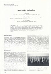
this, we attach water-soaked sponges to the electrodes, <strong>and</strong><br />
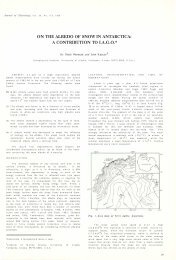
water the immediate vicinity <strong>of</strong> the electrodes (Fig. 1a).<br />
Nevertheless, the currents injected into the ground <strong>and</strong><br />
the measured voltages are generally low. This issue needs to<br />
be considered when selecting the electrode configuration to<br />
be used. Because electrode configurations with low geometrical<br />
factors provide larger voltages (e.g. Reynolds,<br />
1997), Wenner configurations are generally more suitable<br />
for surveying <strong>rock</strong> <strong>glaciers</strong> than dipole–dipole configurations.<br />
Since snow cover may prohibit the current injection,<br />
we prefer to conduct our geoelectric surveys in the summer.<br />
Over the past two decades, tomographic inversion<br />
techniques for geoelectric data have become increasingly<br />
popular <strong>and</strong> user-friendly (http://www.abem.se/). Application<br />
<strong>of</strong> these programs to mountain permafrost data poses no<br />
serious problems so long as they correctly account for the<br />
effects <strong>of</strong> the pronounced topographic relief.<br />
2.3. Seismic techniques<br />
Seismic techniques are mostly sensitive to elastic parameter<br />
variations that govern the propagation speed <strong>of</strong> compressional<br />
waves (P-waves). Characteristic P-wave speeds <strong>of</strong><br />
mountain permafrost materials are quite different (Table 1).<br />
Applications <strong>of</strong> high-resolution seismic techniques require a<br />
relatively large number <strong>of</strong> closely spaced receiver <strong>and</strong><br />
source positions. Typical deployments may include 48–<br />
120 geophones equally spaced at 1–5 m. Ideally, the density<br />
<strong>of</strong> sources should be comparable to that <strong>of</strong> the receivers.<br />
However, to minimize time in the field, the density <strong>of</strong><br />
sources may be substantially less than this.<br />
Surface conditions on <strong>rock</strong> <strong>glaciers</strong> make it difficult to<br />
couple the geophones <strong>and</strong> seismic sources to the ground.<br />
One option is to conduct seismic surveys during the winter.<br />
This alleviates the field effort significantly, but the snow<br />
cover may cause the seismic data to be highly contaminated<br />
with guided phases that obscure the reflections (Musil <strong>and</strong><br />
others, 2002). Our preference is to conduct seismic surveys
112<br />
during the summer. For uniformly good geophone–ground<br />
coupling, we fasten the geophones to the surface boulders<br />
by drilling small holes (Fig. 1b). The extremely heterogeneous<br />
near-surface environment causes substantial attenuation<br />
<strong>of</strong> the seismic waves. Such attenuating conditions<br />
usually preclude the use <strong>of</strong> low-energy sources (e.g.<br />
sledgehammers <strong>and</strong> pipeguns) <strong>and</strong> the difficult terrain<br />
precludes the use <strong>of</strong> mini-vibrators <strong>and</strong> weight-drop devices<br />
(Van der Veen <strong>and</strong> others, 2000). Explosives loaded into<br />
shallow boreholes drilled into the boulders or pushed into<br />
crevices between the boulders provide high levels <strong>of</strong> energy<br />
in a cost-effective manner. To record data over distances <strong>of</strong><br />
100–200 m, charge sizes <strong>of</strong> 100–500 g are necessary.<br />
Near-surface attenuation results in the preferential loss <strong>of</strong><br />
the high-frequency seismic signal. In combination with the<br />
presence <strong>of</strong> strong scattered energy <strong>and</strong> guided phases, this<br />
makes it extremely difficult to image reflections in <strong>rock</strong><br />
glacier seismic data (Musil <strong>and</strong> others, 2002). By comparison,<br />
it is now quite straightforward to extract reliable<br />
information from the first-arriving direct <strong>and</strong> refracted<br />
phases. Although simple analysis techniques (e.g. the<br />
generalized reciprocal method; Palmer, 1980) can be<br />
employed for mapping first-order discontinuities underlying<br />
relatively uniform overburden, more sophisticated 2-D<br />
tomographic inversion techniques are required for analyzing<br />
<strong>rock</strong> glacier seismic data. The geophysical literature describes<br />
tomographic inversion algorithms based on twopoint<br />
ray tracing (Zelt <strong>and</strong> Smith, 1992) <strong>and</strong> finite-difference<br />
Eikonal solvers (Lanz <strong>and</strong> others, 1998), the latter being the<br />
preferred choice for data distinguished by strong lateral<br />
speed variations.<br />
2.4. Georadar surveying<br />
The high electrical resistivity <strong>of</strong> most mountain permafrost<br />
terrains is a positive characteristic for georadar surveying. In<br />
such environments, the georadar techniques are most<br />
sensitive to variations in dielectric permittivity, which govern<br />
the propagation speeds <strong>of</strong> georadar waves. Characteristic<br />
georadar wave speeds in mountain permafrost materials vary<br />
significantly (Table 1).<br />
The high resistivities allow antennas with dominant<br />
frequencies as low as 1 MHz to be employed (Gogenini<br />
<strong>and</strong> others, 1998). For high-resolution investigations, antennas<br />
with dominant frequencies between 20 <strong>and</strong> 100 MHz<br />
have proven to be suitable (Arcone <strong>and</strong> others, 1998; Isaksen<br />
<strong>and</strong> others, 2000; Lehmann <strong>and</strong> Green, 2000; Berthling <strong>and</strong><br />
others, 2003; Moorman <strong>and</strong> others, 2003). Proper coupling<br />
<strong>of</strong> the antennas to the ground is an important prerequisite for<br />
recording high-quality data. This can be realized in winter,<br />
when the snow cover provides uniform surface conditions.<br />
A constant distance between the transmitter <strong>and</strong> receiver<br />
antennas is achieved by mounting both on a single sledge.<br />
Another critical concern in acquiring georadar data is<br />
accurate positioning. High-resolution investigations with<br />
measurement spacings <strong>of</strong> a few tens <strong>of</strong> centimeters require<br />
the use <strong>of</strong> automatic positioning systems (Lehmann <strong>and</strong><br />
Green, 1999; Streich <strong>and</strong> others 2006).<br />
Techniques adopted from seismic reflection data processing<br />
can be used to obtain detailed subsurface images from<br />
the recorded georadar data. Commonly employed processing<br />
steps include amplitude scaling to enhance laterarriving<br />
events relative to the earlier-arriving ones <strong>and</strong><br />
frequency filtering in the time <strong>and</strong> space domains to remove<br />
system noise <strong>and</strong> improve the coherency <strong>of</strong> reflected signals<br />
Maurer <strong>and</strong> Hauck: <strong>Instruments</strong> <strong>and</strong> methods<br />
(Gross <strong>and</strong> others, 2003). If reliable speed information is<br />
available, migration may be used to convert the processed<br />
time sections to equivalent depth sections. To account for<br />
the effects <strong>of</strong> strong topographic relief, special-purpose<br />
topographic migration algorithms may be applied (Lehmann<br />
<strong>and</strong> Green, 2000; Heincke <strong>and</strong> others, 2005).<br />
In small areas (e.g. 50 � 50 m 2 ) <strong>of</strong> particular interest, 3-D<br />
georadar experiments can be performed. This technique has<br />
proven to be highly successful in various applications (Grasmueck<br />
<strong>and</strong> others, 2004; Gross <strong>and</strong> others, 2004; Heincke<br />
<strong>and</strong> others, 2005) <strong>and</strong> is expected to work well on mountain<br />
permafrost. To obtain unaliased subsurface images, it is<br />
critical that the investigation area be very densely sampled.<br />
2.5. Cross-hole methods<br />
Conceptually, most geophysical techniques can also be<br />
applied in a cross-hole mode (e.g. by placing the sources in<br />
one borehole <strong>and</strong> recording the data in another). Cross-hole<br />
tomography provides detailed 2-D information in the plane<br />
containing the two boreholes. The multiple illumination <strong>of</strong><br />
subsurface targets provided by cross-hole geometries results<br />
in more reliable <strong>and</strong> higher-resolution information than can<br />
be provided by most surface-based techniques. Ideally, the<br />
borehole separation should be about half the borehole depth.<br />
Unfortunately, boreholes in mountain permafrost usually<br />
provide less-than-ideal conditions for geophysical experiments<br />
(Arenson <strong>and</strong> others, 2002). The general absence <strong>of</strong><br />
water <strong>and</strong> the presence <strong>of</strong> casing to stabilize the boreholes<br />
may substantially complicate applications <strong>of</strong> certain geophysical<br />
techniques. Diffusive electromagnetic <strong>and</strong> radar<br />
systems can see through PVC casing, but not through metal<br />
casing. For geoelectric surveys, borehole electrodes that can<br />
be operated in dry uncased holes require centralizers with<br />
metal clamping arms. In the presence <strong>of</strong> casing, the<br />
electrodes need to be attached to the outside <strong>of</strong> the casing<br />
before it is inserted into the borehole. To compensate for the<br />
absence <strong>of</strong> water, instead <strong>of</strong> using st<strong>and</strong>ard piezoelectric<br />
sources <strong>and</strong> receivers (i.e. hydrophones) for borehole<br />
seismic experiments, more complicated seismic sources<br />
<strong>and</strong> receivers (i.e. geophones) need to be clamped to the<br />
borehole casing or walls.<br />
3. MURTÈL CASE STUDY<br />
3.1. Site description<br />
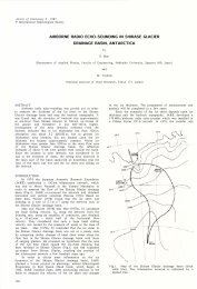
The Murtèl <strong>rock</strong> glacier is located in the Upper Engadine<br />
area <strong>of</strong> the eastern Swiss Alps. It is �150 m wide, 300 m long<br />
<strong>and</strong> extends over an altitude range <strong>of</strong> 2600–2800 m (Fig. 2).<br />
It is moving horizontally a few centimeters per year (Kääb<br />
<strong>and</strong> Weber, 2004). The ongoing movements have generated<br />
numerous flow lobes (Fig. 2). In 1987, a borehole was<br />
drilled to 58 m depth (Vonder Mühll <strong>and</strong> Holub, 1992). It<br />
encountered, at successively greater depths: large boulders<br />
<strong>and</strong> air-filled voids at 0–3 m; an ice-rich layer (more than<br />
40% ice) at 3–15 m; a mixture <strong>of</strong> ice <strong>and</strong> s<strong>and</strong> (30–35% ice)<br />
at 15–30 m: <strong>and</strong> a mixture <strong>of</strong> s<strong>and</strong>s <strong>and</strong> boulders at 30–<br />
52 m, <strong>and</strong> bed<strong>rock</strong> below.<br />
In an attempt to determine the internal structure <strong>of</strong> the<br />
Murtèl <strong>rock</strong> glacier, we recorded TDEM data <strong>and</strong> acquired<br />
surface-based geoelectric, seismic tomographic <strong>and</strong> georadar<br />
data along nearly coincident lines parallel to the <strong>rock</strong><br />
glacier flow direction (Fig. 2). Here, we focus on the<br />
integration <strong>of</strong> information provided by the four datasets.
Maurer <strong>and</strong> Hauck: <strong>Instruments</strong> <strong>and</strong> methods 113<br />
Fig. 1. (a) Galvanic coupling <strong>of</strong> an electrode in the blocky environment<br />
<strong>of</strong> a <strong>rock</strong> glacier. (b) Geophone fastened to a boulder <strong>of</strong> a<br />
<strong>rock</strong> glacier using a small drillhole (yellow stripe at the bottom <strong>of</strong><br />
the image is a measuring tape).<br />
3.2. TDEM survey<br />
TDEM data provided first-order estimates <strong>of</strong> <strong>rock</strong> glacier<br />
thickness (Hauck <strong>and</strong> others, 2001). In principle, this type<br />
<strong>of</strong> information could be obtained directly from the borehole<br />
logs, but to investigate the suitability <strong>of</strong> the TDEM<br />
method on <strong>rock</strong> <strong>glaciers</strong>, a sounding was performed near<br />
the borehole (Hauck <strong>and</strong> others, 2001). Acquisition time<br />
was about half an hour. The TDEM data were inverted<br />
using TEMIX, a commercial s<strong>of</strong>tware package (Interpex<br />
Limited, 1990).<br />
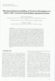
Results <strong>of</strong> the TDEM survey are depicted in Figure 3.<br />
Figure 3a shows the observed data plotted as apparent<br />
resistivity vs time since current turn-<strong>of</strong>f. From the general<br />
shape <strong>of</strong> this curve, we can infer the presence <strong>of</strong> a relatively<br />
resistive layer s<strong>and</strong>wiched between two more conductive<br />
layers, one <strong>of</strong> which approaches the surface. The solid line<br />
in Figure 3b represents the best-fitting model obtained from<br />
the inversion program, <strong>and</strong> the gray shaded area represents<br />
‘equivalent’ models that explain the data nearly as well as<br />
the best-fitting model (Nabighian <strong>and</strong> Macnae, 1987). The<br />
significant decrease <strong>of</strong> resistivity at 54 � 15 m depth coincides<br />
with the <strong>rock</strong>-glacier–bed<strong>rock</strong> interface.<br />
3.3. Tomographic geoelectric survey<br />
We made 103 Wenner geoelectric measurements along a<br />
145 m long pr<strong>of</strong>ile across the frontal region <strong>of</strong> the <strong>rock</strong><br />
Fig. 2. (a) Photograph <strong>of</strong> the Murtèl <strong>rock</strong> glacier. View direction is<br />
indicated with a black arrow in (b). (b) Orthophoto <strong>of</strong> the Murtèl<br />
<strong>rock</strong> glacier showing the locations <strong>of</strong> the borehole (black dot) <strong>and</strong><br />
the geoelectric (blue), seismic (red) <strong>and</strong> georadar (magenta) pr<strong>of</strong>iles.<br />
glacier (Fig. 2), deploying 30 electrodes equally spaced at<br />
5 m intervals. Electrode coupling was especially difficult on<br />
this <strong>rock</strong> glacier, because the surface consisted <strong>of</strong> large<br />
boulders (up to 2 m high) with only small amounts <strong>of</strong> finegrained<br />
material. The total acquisition time was 5 hours. Our<br />
geoelectric data were tomographically inverted using<br />
RES2DINV, a commercial s<strong>of</strong>tware package (http://www.<br />
abem.se/).<br />
A moderately conductive near-surface layer (DC1) with a<br />
resistivity <strong>of</strong> �10 k� m <strong>and</strong> a thickness <strong>of</strong> about �2.5 m is<br />
observed along the length <strong>of</strong> the recording line (Fig. 4a; DC1<br />
in Fig. 4c). Within the <strong>rock</strong> glacier, i.e. below DC1, in the<br />
horizontal distance range 50–140 m, the resistivity increases<br />
abruptly to the M� m range. At about 140 m horizontal<br />
distance, near where the surface exposure <strong>of</strong> the <strong>rock</strong> glacier<br />
ends, resistivities at depth change from the M� m range to<br />
the k� m range across a steeply dipping boundary denoted<br />
as DC2 in Figure 4c.<br />
3.4. Tomographic seismic survey<br />
Our tomographic seismic experiment across the Murtèl <strong>rock</strong><br />
glacier was conducted during the summer. Using a 120channel<br />
seismograph, 120 geophones spaced at 2 m intervals
114<br />
Fig. 3. Results <strong>of</strong> a TDEM sounding on the Murtèl <strong>rock</strong> glacier.<br />
(a) The observed (squares) <strong>and</strong> predicted (solid line) data based on<br />
the best-fitting model shown by the solid line in (b). Gray shaded<br />
area in (b) indicates the range <strong>of</strong> equivalent models that explain the<br />
data nearly as well as the best-fitting model.<br />
<strong>and</strong> 44 sources (charges <strong>of</strong> 200–400 g) spaced at �5.4 m<br />
intervals, we acquired data along a 238 m long pr<strong>of</strong>ile. Four<br />
days were required to record the data. Data inversion was<br />
performed using the tomographic program described by Lanz<br />
<strong>and</strong> others (1998).<br />
The resulting speed tomogram contains three principal<br />
units (Fig. 4b <strong>and</strong> d). A laterally extensive surface layer, S1,<br />
with speeds 4000 m s –1 . The interface between the middle <strong>and</strong> lower<br />
units is labeled S2 in Figure 4d. At a horizontal distance <strong>of</strong><br />
�90 m, an isolated high-speed feature is observed immediately<br />
below the low-speed surface layer (S3 in Fig. 4d).<br />
Although the spatial extent <strong>of</strong> S3 is quite small, it appeared in<br />
all our inversion runs using different initial models <strong>and</strong><br />
regularization parameters. The frontal part <strong>of</strong> the <strong>rock</strong> glacier<br />
exhibits pronounced speed contrasts, with a 10–15 m thick<br />
surface block <strong>of</strong> very low-speed material overlying <strong>rock</strong>s with<br />
speeds >5000 m s –1 .<br />
3.5. Georadar survey<br />
We used 50 MHz antennas <strong>and</strong> a station spacing <strong>of</strong> 0.5 m to<br />
record georadar data along a �350 m long pr<strong>of</strong>ile (Fig. 2b).<br />
A relatively simple processing scheme that included automatic<br />
gain control, frequency filtering, spectral whitening<br />
<strong>and</strong> F-X deconvolution was applied to the data. Unfortunately,<br />
no detailed speed information was available along<br />
the pr<strong>of</strong>ile, which precluded us from applying topographic<br />
migration. Instead, we performed a simple time-to-depth<br />
conversion using a speed <strong>of</strong> 120 m ms –1 (based on a<br />
common-midpoint measurement in the central part <strong>of</strong> the<br />
<strong>rock</strong> glacier). Appraisal <strong>of</strong> a depth error associated with the<br />
overly simplified assumption <strong>of</strong> a homogeneous speed is<br />
difficult, but we judge that depth errors should not exceed<br />
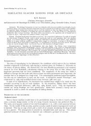
10%. The final section is displayed in Figure 5. Maximum<br />
depth penetration <strong>of</strong> the georadar signals is about 50 m.<br />
Several prominent dipping reflections extend over substantial<br />
portions <strong>of</strong> the pr<strong>of</strong>ile (highlighted by black lines in<br />
Fig. 5b).<br />
Maurer <strong>and</strong> Hauck: <strong>Instruments</strong> <strong>and</strong> methods<br />
Fig. 4. (a, b) Results from the (a) geoelectric <strong>and</strong> (b) seismic surveys<br />
conducted on the Murtèl <strong>rock</strong> glacier. (c, d) Our interpretations<br />
superimposed on the tomograms <strong>of</strong> (a) <strong>and</strong> (b) respectively.<br />
Topography defined by the coordinates <strong>of</strong> the geophones is<br />
superimposed on all sections. Location <strong>of</strong> the pr<strong>of</strong>ile is shown in<br />
Figure 2. Frontal part <strong>of</strong> the <strong>rock</strong> glacier is marked in all panels with<br />
a black arrow. DC1 <strong>and</strong> S1 denote the active layer, DC2 is the<br />
boundary between frozen <strong>and</strong> unfrozen material, S2 is the bed<strong>rock</strong><br />
interface <strong>and</strong> S3 is probably a huge boulder.<br />
3.6. Integrated interpretation<br />
Figure 6 shows a sketch <strong>of</strong> our interpretation <strong>of</strong> important<br />
features identified in the geoelectric, seismic <strong>and</strong> georadar<br />
images. Our interpretation is constrained by information<br />
provided by the borehole. The nearly coincident DC1 <strong>and</strong><br />
S1 layers represent the bottom <strong>of</strong> the active layer, which<br />
melts in the summer <strong>and</strong> freezes in the winter. This active<br />
layer, which corresponds to loose boulders at the top <strong>of</strong> the<br />
borehole, has moderate resistivities <strong>of</strong> �10 k� m <strong>and</strong> low<br />
seismic speeds <strong>of</strong>
Maurer <strong>and</strong> Hauck: <strong>Instruments</strong> <strong>and</strong> methods 115<br />
Fig. 5. (a) Georadar section recorded along the Murtèl <strong>rock</strong> glacier. (b) Our interpretation superimposed on the georadar section. Location <strong>of</strong><br />
the pr<strong>of</strong>ile is shown in Figure 2.<br />
The series <strong>of</strong> reflections observed in the up-glacier part <strong>of</strong><br />
the georadar section (Fig. 5) are most likely to originate from<br />
alternating snow <strong>and</strong> debris accumulations created by mass<br />
movement events from the slope above the <strong>rock</strong> glacier.<br />
Such features are quite common in georadar images <strong>of</strong> the<br />
upper part <strong>of</strong> <strong>rock</strong> <strong>glaciers</strong>; they represent the snow <strong>and</strong><br />
debris sources that define the typical morphology <strong>of</strong> <strong>rock</strong><br />
glacier bodies (e.g. Berthling <strong>and</strong> others, 2003). In the<br />
central <strong>and</strong> down-glacier parts <strong>of</strong> the georadar section, the<br />
two dominant reflections originate from the ice-rich <strong>and</strong><br />
moderately ice-rich layers observed in the borehole (reflection<br />
intersects the borehole at the boundary between icerich<br />
<strong>and</strong> s<strong>and</strong> <strong>and</strong> ice layers; Fig. 6). The deeper reflection at<br />
�20–30 m depth between 0 <strong>and</strong> 125 m distance corresponds<br />
to the bottom <strong>of</strong> the ice-containing units <strong>and</strong> to the<br />
shear horizon observed in the inclinometer measurements<br />
described by Vonder Mühll <strong>and</strong> Holub (1992). Their<br />
measurements indicate displacement rates <strong>of</strong> 0.04 m a –1 at<br />
this depth.<br />
The seismic speed discontinuity, S2, in Figure 4d defines<br />
the top <strong>of</strong> the bed<strong>rock</strong>. Towards the frontal part <strong>of</strong> the <strong>rock</strong><br />
glacier, S2 becomes shallower, reaching the surface at about<br />
170 m horizontal distance. The high bed<strong>rock</strong> speeds within<br />
this bed<strong>rock</strong> protrusion may indicate the presence <strong>of</strong><br />
virtually unfractured <strong>rock</strong> that may have acted as a barrier<br />
to the flow <strong>of</strong> the <strong>rock</strong> glacier.<br />
4. MURAGL CASE STUDY<br />
4.1. Site description<br />
The Muragl <strong>rock</strong> glacier is also located in the Upper<br />
Engadine area. It is 100–300 m wide, �700 m long <strong>and</strong><br />
extends over an altitude range <strong>of</strong> 2600–2800 m (Fig. 7). It is<br />
distinguished by rapid horizontal movements <strong>of</strong> up to<br />
0.5 m a –1 (Kääb <strong>and</strong> Vollmer, 2000). This is substantially<br />
faster than typical <strong>rock</strong> glacier movements, which are <strong>of</strong> the<br />
order <strong>of</strong> several cm a –1 . Like the Murtèl <strong>rock</strong> glacier, it exhibits<br />
pronounced flow lobes with transverse furrows <strong>and</strong><br />
ridges. The irregular flow-lobe pattern <strong>of</strong> the Muragl <strong>rock</strong><br />
glacier (compare Fig. 7b with Fig. 2b) may be the result <strong>of</strong><br />
periodic mass movements, perhaps reflecting several generations<br />
<strong>of</strong> <strong>rock</strong> glacier evolution. In 1999, four boreholes,<br />
B1–B4, were drilled through the <strong>rock</strong> glacier to bed<strong>rock</strong><br />
Fig. 6. Integrated interpretation <strong>of</strong> boundaries observed in the<br />
geoelectric (blue lines), seismic (red lines) <strong>and</strong> georadar (magenta<br />
lines) images from the Murtèl <strong>rock</strong> glacier. The borehole log is also<br />
displayed. DC1 <strong>and</strong> S1 denote the active layer, DC2 is the boundary<br />
between frozen <strong>and</strong> unfrozen material, S2 is the bed<strong>rock</strong> interface<br />
<strong>and</strong> S3 is probably a huge boulder.
116<br />
Fig. 7. (a) Photograph <strong>of</strong> the Muragl <strong>rock</strong> glacier. View direction is<br />
indicated with a black arrow in (b). (b) Orthophoto <strong>of</strong> the Muragl<br />
<strong>rock</strong> glacier showing the locations <strong>of</strong> the boreholes (black dots), the<br />
surface geoelectric (blue) <strong>and</strong> seismic (red) pr<strong>of</strong>iles <strong>and</strong> the crosshole<br />
georadar (magenta) sections.<br />
(Arenson <strong>and</strong> others, 2002; Fig. 7b). A more detailed<br />
description <strong>of</strong> the borehole logs is deferred to section 4.5,<br />
but the geology at progressively greater depths can be<br />
described as: (i) loose boulders, (ii) a mixture <strong>of</strong> s<strong>and</strong>,<br />
boulders <strong>and</strong> ice, (iii) a zone <strong>of</strong> boulders <strong>and</strong> voids, (iv) s<strong>and</strong><br />
that is mostly free <strong>of</strong> ice <strong>and</strong> (v) bed<strong>rock</strong> at 32–45 m depth.<br />
Thin water-saturated zones are found within the core <strong>of</strong> the<br />
<strong>rock</strong> glacier.<br />
One goal <strong>of</strong> our project was to compare the internal<br />
structures <strong>of</strong> the slow-moving Murtèl <strong>and</strong> fast-moving<br />
Muragl <strong>rock</strong> <strong>glaciers</strong>. Accordingly, we attempted to collect<br />
similar datasets at the two study sites. Unfortunately, the<br />
surface-based georadar <strong>and</strong> TDEM sounding data collected<br />
across the Muragl <strong>rock</strong> glacier did not yield useful<br />
information, possibly as a result <strong>of</strong> scattering <strong>and</strong> absorption<br />
<strong>of</strong> the electromagnetic energy within a more complex <strong>rock</strong><br />
glacier mass. In contrast, the surface geoelectric <strong>and</strong> seismic<br />
surveys <strong>and</strong> the cross-hole radar experiments produced<br />
many useful data. For logistic reasons, we could only collect<br />
data along the axis <strong>of</strong> the Murtèl <strong>rock</strong> glacier (Fig. 2b) <strong>and</strong><br />
along a direction perpendicular to the axis <strong>of</strong> the Muragl<br />
<strong>rock</strong> glacier (Fig. 7b).<br />
Fig. 8. Results from the (a) geoelectric, (b) seismic <strong>and</strong> (c) cross-hole<br />
georadar surveys conducted on the Muragl <strong>rock</strong> glacier. Topography<br />
defined by the coordinates <strong>of</strong> the geophones is superimposed<br />
on (a) <strong>and</strong> (b). Note that geoelectric data were acquired in summer<br />
<strong>and</strong> seismic data were recorded in winter. Differences in topography<br />
are caused by the snow cover during the seismic campaign.<br />
Locations <strong>of</strong> the surveys are shown in Figure 7.<br />
4.2. Tomographic geoelectric survey<br />
We employed very similar recording parameters <strong>and</strong><br />
identical data inversion s<strong>of</strong>tware for the Murtèl <strong>and</strong> Muragl<br />
<strong>rock</strong> glacier investigations. The resultant uninterpreted <strong>and</strong><br />
interpreted resistivity tomograms for the Muragl <strong>rock</strong> glacier<br />
are shown in Figures 8a <strong>and</strong> 9a, respectively.<br />
A thin layer <strong>of</strong> moderately high-resistivity material<br />
underlies the undulating surface (DC1 in Fig. 9a). This is<br />
underlain in the southwest part <strong>of</strong> the survey line by higherresistivity<br />
material (several tens <strong>of</strong> k� m; DC2 in Fig. 9a).<br />
Within DC2, there is a highly resistive core with resistivities<br />
in the M� m range (DC3 in Fig. 9a). The remaining regions<br />
<strong>of</strong> the tomogram have resistivities <strong>of</strong> several k� m.<br />
4.3. Tomographic seismic survey<br />
Maurer <strong>and</strong> Hauck: <strong>Instruments</strong> <strong>and</strong> methods<br />
In contrast to the Murtèl field campaign, we acquired our<br />
seismic data across the Muragl <strong>rock</strong> glacier during the winter.<br />
Geophones were planted in a compacted layer <strong>of</strong> surface<br />
snow, <strong>and</strong> the dynamite charges were placed 1–2 m beneath<br />
the surface at the base <strong>of</strong> the snow layer. Technical details <strong>of</strong><br />
the seismic data acquisition <strong>and</strong> processing are given by<br />
Musil <strong>and</strong> others (2002). We again used a 120-channel<br />
seismograph, but the 120 geophones were spaced at 2.5 m
Maurer <strong>and</strong> Hauck: <strong>Instruments</strong> <strong>and</strong> methods 117<br />
Fig. 9. As for Figure 8, but with our interpretations superimposed on<br />
the tomograms. The borehole logs are also displayed. DC1 <strong>and</strong> S1<br />
represent the active layer, DC3 is the ice-rich core <strong>of</strong> the <strong>rock</strong><br />
glacier, S2 represents degraded permafrost <strong>and</strong> S3 is the bed<strong>rock</strong><br />
interface. R1 represents an ice-rich zone, R2 is a layer with large<br />
voids, R3 is either ice-rich or includes voids (see text) <strong>and</strong> R4 is the<br />
water-saturated part <strong>of</strong> the <strong>rock</strong> glacier.<br />
intervals <strong>and</strong> the 53 sources were separated from each other<br />
by �5.6 m. The total pr<strong>of</strong>ile length was 297.5 m (Fig. 7).<br />
The resultant tomographic seismic image in Figure 8b is<br />
characterized by pronounced variations <strong>of</strong> seismic speed.<br />
A 5–10 m thick surface layer <strong>of</strong> low-speed material extends<br />
the length <strong>of</strong> the line (S1 in Fig. 9b). Between 160 <strong>and</strong> 200 m<br />
horizontal distance, low speeds can be traced to even<br />
greater depths (low-speed body S2 in Fig. 9b). Towards both<br />
ends <strong>of</strong> the pr<strong>of</strong>ile, speeds immediately below the nearsurface<br />
low-speed layer are >4000 m s –1 . Speeds are uniformly<br />
>4000 m s –1 along the base <strong>of</strong> the entire image<br />
(interface S3 in Fig. 9b delineates approximately the upper<br />
boundary <strong>of</strong> speeds >4000 m s –1 ).<br />
4.4. Cross-hole radar survey<br />
Using low-frequency (22 MHz) transmitter <strong>and</strong> receiver<br />
antennas (�3 m long), cross-hole radar data were collected<br />
between boreholes B4 <strong>and</strong> B1 <strong>and</strong> between B4 <strong>and</strong> B2.<br />
Transmitter <strong>and</strong> receiver spacings were both 1 m. Tomographic<br />
inversions <strong>of</strong> the travel-time data were performed<br />
using an algorithm described by Maurer <strong>and</strong> Green (1997).<br />
Further details <strong>of</strong> the experiment can be found in Musil <strong>and</strong><br />
others (2006).<br />
Perspective images <strong>of</strong> the tomographic planes B4–B1 <strong>and</strong><br />
B4–B2 are shown in Figures 8c <strong>and</strong> 9c. They are<br />
characterized by a background speed <strong>of</strong> �120 m ms –1 <strong>and</strong><br />
Fig. 10. Integrated interpretation <strong>of</strong> geoelectric (blue lines) <strong>and</strong><br />
seismic (red lines) images from the Muragl <strong>rock</strong> glacier. The borehole<br />
logs <strong>of</strong> B1 <strong>and</strong> B2 are also displayed. DC1 <strong>and</strong> S1 represent the<br />
active layer, DC3 is the ice-rich core <strong>of</strong> the <strong>rock</strong> glacier, S2<br />
represents degraded permafrost <strong>and</strong> S3 is the bed<strong>rock</strong> interface.<br />
imbedded zones <strong>of</strong> both higher <strong>and</strong> lower speed. At depths<br />
<strong>of</strong>
118<br />
Table 2. Summary <strong>of</strong> key results from the investigations performed on the Murtèl <strong>and</strong> Muragl <strong>rock</strong> <strong>glaciers</strong> (n.a. ¼ not applied, n.s. ¼ not<br />
successful)<br />
Rock glacier TDEM Geoelectrics Seismic refraction<br />
tomography<br />
Murtèl Approximate<br />
bed<strong>rock</strong> depth<br />
Active layer, ice content,<br />
structure <strong>of</strong> frontal part<br />
Muragl n.s. Active layer, ice content,<br />
partially bed<strong>rock</strong> depth<br />
3-D effects, with the seismic energy having traveled out-<strong>of</strong>the-plane<br />
<strong>of</strong> the pr<strong>of</strong>ile along a slightly shallower region <strong>of</strong><br />
bed<strong>rock</strong>. The correlation between the lower boundary <strong>of</strong> the<br />
high-resistivity region DC2 <strong>and</strong> S3 varies from good at<br />
horizontal distances 40–70 m to poor at shorter <strong>and</strong> longer<br />
distances. Based on the air photograph in Figure 7b, we<br />
judge that S3 represents reasonably well the depth to<br />
bed<strong>rock</strong> beneath the southwest end <strong>of</strong> the line.<br />
Radar features R1–R4 are not included in Figure 10, because<br />
the cross-hole tomographic planes are highly oblique<br />
to the plane containing the geoelectric <strong>and</strong> seismic tomograms<br />
(Fig. 7b). Nevertheless, a comparison <strong>of</strong> Figures 9c<br />
<strong>and</strong> 10 reveals some interesting correlations. For example,<br />
the high-speed zone, R1, coincides with the northeast lobe<br />
<strong>of</strong> the high-resistivity region, DC2, in which the pores<br />
between the sediments <strong>and</strong> boulders are filled with ice (see<br />
the ice-rich zones in the B2 <strong>and</strong> B4 borehole logs; Fig. 9c),<br />
whereas the underlying high-speed zone, R2, is located in a<br />
lower-resistivity region in which the pores are mostly empty<br />
(see the loose boulders <strong>and</strong> dry ice-free s<strong>and</strong>s at the<br />
appropriate depths in the B2 <strong>and</strong> B4 borehole logs;<br />
Fig. 9c). These observations are entirely consistent with the<br />
relatively high radar speeds <strong>of</strong> ice (170 m ms –1 ) <strong>and</strong> air<br />
(300 m ms –1 ) <strong>and</strong> with the joint interpretations <strong>of</strong> georadar<br />
travel times <strong>and</strong> amplitudes <strong>of</strong> Musil <strong>and</strong> others (2006). To<br />
generate the high speeds observed in R2, the air voids must<br />
be quite large. Since it is not possible to maintain such voids<br />
in an active <strong>rock</strong> glacier over long periods, they were<br />
probably filled with ice until quite recently (Musil <strong>and</strong><br />
others, 2006).<br />
Interpretation <strong>of</strong> the high-speed zone, R3, is not<br />
conclusive. It could represent a zone with pores filled with<br />
ice or air. Since R3 extends close to borehole B1, which is<br />
situated within degraded permafrost, we prefer the option <strong>of</strong><br />
air-filled voids. Finally, the low speeds <strong>of</strong> zone R4 may be<br />
associated with one or more water-bearing layers intersected<br />
in boreholes B1, B2 <strong>and</strong> B4 (Musil <strong>and</strong> others, 2006). There<br />
is no perfect correlation between the borehole logs <strong>and</strong> the<br />
tomograms. This may be the result <strong>of</strong> alterations caused by<br />
the drilling process.<br />
Comparisons <strong>of</strong> the radar tomographic images with the<br />
results <strong>of</strong> inclinometer measurements performed in borehole<br />
B4 (Arenson <strong>and</strong> others, 2002) reveal an interesting similarity<br />
with the Murtèl <strong>rock</strong> glacier. As indicated by the black<br />
arrow in Figure 9c, most <strong>of</strong> the displacements are<br />
concentrated at the bottom <strong>of</strong> the ice-rich layer defined by<br />
the high-speed zone, R1. The much higher displacement<br />
rates at the Muragl <strong>rock</strong> glacier relative to those at the Murtèl<br />
<strong>rock</strong> glacier may be the result <strong>of</strong> generally higher temperatures<br />
close to the melting point <strong>of</strong> ice, as measured in the<br />
boreholes (Vonder Mühll <strong>and</strong> others, 2005).<br />
Active layer, large blocks,<br />
bed<strong>rock</strong> depth<br />
Active layer, degraded<br />
permafrost, bed<strong>rock</strong> depth<br />
Maurer <strong>and</strong> Hauck: <strong>Instruments</strong> <strong>and</strong> methods<br />
Surface georadar Borehole georadar<br />
Detailed internal<br />
structure <strong>of</strong> <strong>rock</strong> glacier<br />
5. CONCLUSIONS AND OUTLOOK<br />
n.a.<br />
n.s. Ice-rich zones, voids,<br />
water content<br />
Our investigations <strong>of</strong> two <strong>alpine</strong> <strong>rock</strong> <strong>glaciers</strong> have demonstrated<br />
some <strong>of</strong> the possibilities <strong>and</strong> some <strong>of</strong> the limitations<br />
<strong>of</strong> applying high-resolution geophysical techniques in such<br />
environments. We have shown that it is generally feasible to<br />
obtain meaningful 2-D subsurface images, despite the<br />
extremely challenging data acquisition conditions. Several<br />
newly mapped features provide fresh insights into the<br />
stability, kinematics <strong>and</strong> dynamics <strong>of</strong> the <strong>rock</strong> <strong>glaciers</strong><br />
(Table 2). Key results include the:<br />
locations <strong>and</strong> geometries <strong>of</strong> the active layers <strong>and</strong> bed<strong>rock</strong><br />
surface,<br />
characterization <strong>of</strong> the Murtèl <strong>rock</strong> glacier frontal zone,<br />
spatial distributions <strong>of</strong> ice-, water- <strong>and</strong> air-filled voids in<br />
the Muragl <strong>rock</strong> glacier,<br />
delineation <strong>of</strong> internal structures such as shear zones.<br />
Another important conclusion <strong>of</strong> our studies is that geoelectric,<br />
seismic <strong>and</strong> georadar data provide both redundant<br />
<strong>and</strong> complementary information. For example, ice-rich<br />
zones are best delineated on the basis <strong>of</strong> their very high<br />
electrical resistivities, whereas interfaces between loose <strong>and</strong><br />
more compacted material (e.g. the base <strong>of</strong> the active layer,<br />
regions <strong>of</strong> degraded permafrost, the top <strong>of</strong> the bed<strong>rock</strong>) are<br />
best seen in seismic images. Surface-based georadar was the<br />
only method that allowed shear horizons to be determined,<br />
<strong>and</strong> borehole radar tomography revealed the presence <strong>of</strong><br />
small-scale structures that were essentially invisible to the<br />
surface-based techniques.<br />
For future investigations <strong>of</strong> <strong>rock</strong> <strong>glaciers</strong> or other<br />
mountainous regions underlain by permafrost we suggest<br />
the following template:<br />
1. Use the fast <strong>and</strong> inexpensive (i) TDEM method to provide<br />
initial information on the gross (1-D) internal structures<br />
<strong>of</strong> the <strong>rock</strong> <strong>glaciers</strong> <strong>and</strong> their surroundings <strong>and</strong><br />
(ii) surface-based georadar method to obtain detailed<br />
2-D images <strong>of</strong> the same features.<br />
2. On the basis <strong>of</strong> the TDEM soundings <strong>and</strong> georadar<br />
images, select appropriate locations <strong>and</strong> electrode<br />
spacings for acquiring multi-electrode geoelectric data<br />
along one or more pr<strong>of</strong>iles. Very-high-resistivity regions<br />
<strong>of</strong> the resultant electrical resistivity tomogram may<br />
delineate the spatial distribution <strong>of</strong> ice.<br />
3. Depending on the available funds <strong>and</strong> the level <strong>of</strong><br />
information required, it may be useful to collect seismic<br />
data. If bed<strong>rock</strong> topography is the target <strong>of</strong> primary<br />
interest, seismic data are essential. The geoelectric,
Maurer <strong>and</strong> Hauck: <strong>Instruments</strong> <strong>and</strong> methods 119<br />
seismic <strong>and</strong> georadar data should be recorded along<br />
common pr<strong>of</strong>iles.<br />
4. Based on the knowledge acquired as a result <strong>of</strong> steps 1–<br />
3, one or more boreholes should be drilled to groundtruth<br />
<strong>and</strong>/or calibrate the geophysical tomograms.<br />
5. Considering the high costs <strong>of</strong> drilling, it is almost always<br />
worthwhile to record cross-hole <strong>and</strong>/or borehole-tosurface<br />
datasets. Choice <strong>of</strong> the data type (i.e. diffusive<br />
electromagnetic, geoelectric, seismic or georadar) depends<br />
on the problem.<br />
6. In areas <strong>of</strong> particular interest (identified from the results<br />
<strong>of</strong> applying steps 1–5), small-scale 3-D georadar experiments<br />
may be performed.<br />
ACKNOWLEDGEMENTS<br />
This project would not have been feasible without the<br />
involvement <strong>of</strong> many people. We thank M. Musil, L. Arenson,<br />
S. Springman, D. Vonder Mühll, C. Kneisel, C. Baerlocher,<br />
M. Sperl, A. Seward, S. Metzger, H. Horstmeyer, T. Richter<br />
<strong>and</strong> the numerous field helpers for all their contributions.<br />
Financial support was provided by ETH Zürich (grant<br />
No. 0-20535), the EC project PACE <strong>and</strong> Academia Engadina.<br />
We thank A. Green for discussions <strong>and</strong> his thorough inhouse<br />
review <strong>of</strong> the manuscript, which improved the quality<br />
<strong>of</strong> the paper substantially. Finally we acknowledge the<br />
helpful comments <strong>of</strong> reviewer B. Kulessa <strong>and</strong> an anonymous<br />
reviewer.<br />
REFERENCES<br />
Arcone, S.A., D.E. Lawson, A.J. Delaney, J.C. Strasser <strong>and</strong><br />
J.D. Strasser. 1998. Ground-penetrating radar reflection pr<strong>of</strong>iling<br />
<strong>of</strong> groundwater <strong>and</strong> bed<strong>rock</strong> in an area <strong>of</strong> discontinuous<br />
permafrost. Geophysics, 63(5), 1573–1584.<br />
Arenson, L., M. Hoelzle <strong>and</strong> S. Springman. 2002. Borehole<br />
deformation measurements <strong>and</strong> internal structure <strong>of</strong> some <strong>rock</strong><br />
<strong>glaciers</strong> in Switzerl<strong>and</strong>. Permafrost Periglac. Process, 13(2),<br />
117–135.<br />
Berthling, I., B. Etzelmüller, M. Wa˚le <strong>and</strong> J.L. Sollid. 2003. Use <strong>of</strong><br />
Ground Penetration Radar (GPR) soundings for investigating<br />
internal structures in <strong>rock</strong> <strong>glaciers</strong>. Examples from Prins Karls<br />
Forl<strong>and</strong>, Svalbard. Z. Geomorphol., Supplementb<strong>and</strong> 132,<br />
103–121.<br />
Beylich, A.A. <strong>and</strong> 6 others. 2003. Assessment <strong>of</strong> chemical<br />
denudation rates using hydrological measurements, water<br />
chemistry analysis <strong>and</strong> electromagnetic geophysical data.<br />
Permafrost Periglac. Process, 14(4), 387–397.<br />
Bucki, A.K., K.A. Echelmeyer <strong>and</strong> S. MacInnes. 2004. The thickness<br />
<strong>and</strong> internal structure <strong>of</strong> Fireweed <strong>rock</strong> glacier, Alaska,<br />
USA as determined by geophysical methods. J. Glaciol.,<br />
50(168), 67–75.<br />
Davies, M.C.R., O. Hamza <strong>and</strong> C. Harris. 2001. The effect <strong>of</strong> rise in<br />
mean annual air temperature on the stability <strong>of</strong> <strong>rock</strong> slopes<br />
containing ice-filled discontinuities. Permafrost Periglac. Process,<br />
12(1), 137–144.<br />
Fischer, L., A. Kääb, C. Huggel <strong>and</strong> J. Nötzli. 2005. Geology, glacier<br />
changes, permafrost <strong>and</strong> related slope instabilities in a highmountain<br />
<strong>rock</strong> face: Monte Rosa east face, Italian Alps.<br />
Geophys. Res. Abstr., 7, 00518.<br />
Gogineni, S., T. Chuah, C. Allen, K. Jezek <strong>and</strong> R.K. Moore. 1998.<br />
An improved coherent radar depth sounder. J. Glaciol., 44(148),<br />
659–669.<br />
Grasmueck, M., R. Weger <strong>and</strong> H. Horstmeyer. 2004. Threedimensional<br />
ground-penetrating radar <strong>imaging</strong> <strong>of</strong> sedimentary<br />
structures, fractures, <strong>and</strong> archaeological features at submeter<br />
resolution. Geology, 32(11), 933–936.<br />
Gross, R., A. Green, H. Horstmeyer, K. Holliger <strong>and</strong> J. Baldwin.<br />
2003. 3-D georadar images <strong>of</strong> an active fault: efficient data<br />
acquisition, processing <strong>and</strong> interpretation strategies. Subsurf.<br />
Sens. Technol. Appl., 4(1), 19–40.<br />
Gross, R., A.G. Green, H. Horstmeyer <strong>and</strong> J.H. Begg. 2004.<br />
Location <strong>and</strong> geometry <strong>of</strong> the Wellington Fault (New Zeal<strong>and</strong>)<br />
defined by detailed three-dimensional georadar data.<br />
J. Geophys. Res., 109(B5), B05401. (10.1029/2003JB002615.)<br />
Gruber, S., M. Hoelzle <strong>and</strong> W. Haeberli. 2004. Permafrost thaw <strong>and</strong><br />
destabilization <strong>of</strong> Alpine <strong>rock</strong> walls in the hot summer <strong>of</strong> 2003.<br />
Geophys. Res. Lett., 31(13), L13504. (10.1029/2004GL020051.)<br />
Haeberli, W. 1992. Construction, environmental problems <strong>and</strong><br />
natural hazards in periglacial mountain belts. Permafrost<br />
Periglac. Process., 3(2), 111–124.<br />
Harris, C. <strong>and</strong> 9 others. 2003. Warming permafrost in European<br />
mountains. Global Planet. Change, 39(3–4), 215–225.<br />
Hauck, C. <strong>and</strong> D. Vonder Mühll. 2003. Using DC resistivity<br />
tomography to detect <strong>and</strong> characterise mountain permafrost.<br />
Geophys. Prospect., 51(4), 273–284.<br />
Hauck, C., M. Guglielmin, K. Isaksen <strong>and</strong> D. Vonder Mühll. 2001.<br />
Applicability <strong>of</strong> frequency domain <strong>and</strong> time-domain electromagnetic<br />
methods. Permafrost Periglac. Process, 12(1), 39–52.<br />
Hauck, C., K. Isaksen, D.S. Vonder Mühll <strong>and</strong> J.L. Sollid. 2004.<br />
<strong>Geophysical</strong> surveys designed to delineate the altitudinal limit<br />
<strong>of</strong> mountain permafrost: an example from Jotunheimen, Norway.<br />
Permafrost Periglac. Process, 15(3), 191–205.<br />
Heggem, E.S.F., H. Juliussen <strong>and</strong> B. Etzelmüller. 2005. Mountain<br />
permafrost in Central-Eastern Norway. Nor. Geogr, Tidsskr.<br />
59(2), 94–108.<br />
Heincke, B., A.G. Green, J. van der Kruk <strong>and</strong> H. Horstmeyer. 2005.<br />
Acquisition <strong>and</strong> processing strategies for 3D georadar surveying<br />
a region characterized by rugged topography. Geophysics, 70(6),<br />
K53–K61.<br />
Hoekstra, P. 1978. Electromagnetic methods for mapping shallow<br />
permafrost. Geophysics, 43(4), 782–787.<br />
Interpex Limited. 1990. TEMIX user’s manual. Golden, CO,<br />
Interpex Limited.<br />
Isaksen, K., R.S. Ödega˚rd, T. Eiken <strong>and</strong> J.L. Sollid. 2000. Composition,<br />
flow <strong>and</strong> development <strong>of</strong> two tongue-shaped <strong>rock</strong><br />
<strong>glaciers</strong> in the permafrost <strong>of</strong> Svalbard. Permafrost Periglac.<br />
Process, 11 (3), 241–257.<br />
Ishikawa, M., T. Watanabe <strong>and</strong> N. Nakamura. 2001. Genetic<br />
difference <strong>of</strong> <strong>rock</strong> <strong>glaciers</strong> <strong>and</strong> the discontinuous mountain<br />
permafrost zone in Kanchanjunga Himal, Eastern Nepal.<br />
Permafrost Periglac. Process, 12(3), 243–253.<br />
Kääb, A. <strong>and</strong> M. Vollmer. 2000. Surface geometry, thickness<br />
changes <strong>and</strong> flow fields on permafrost streams: automatic<br />
extraction by digital image analysis. Permafrost Periglac.<br />
Process, 11(4), 315–326.<br />
Kääb, A. <strong>and</strong> M. Weber. 2004. Development <strong>of</strong> transverse ridges on<br />
<strong>rock</strong> <strong>glaciers</strong>: field measurements <strong>and</strong> laboratory experiments.<br />
Permafr. Periglac. Proc., 15, 379–391.<br />
Kneisel, C. 2004. New insights into mountain permafrost occurrence<br />
<strong>and</strong> characteristics in glacier forefields at high altitude<br />
through the application <strong>of</strong> 2D resistivity <strong>imaging</strong>. Permafrost<br />
Periglac. Process, 15(3), 221–227.<br />
Kneisel, C., C. Hauck <strong>and</strong> D.S. Vonder Mühll. 2000. Permafrost<br />
below the timberline confirmed <strong>and</strong> characterized by geoelectrical<br />
resistivity measurements, Bever Valley, eastern Swiss Alps.<br />
Permafrost Periglac. Process, 11, 295–304.<br />
Lanz, E., H.R. Maurer, A.G. Green <strong>and</strong> J. Ansorge. 1998. Refraction<br />
tomography over a buried waste disposal site. Geophysics,<br />
63(4), 1414–1433.<br />
Lehmann, F. <strong>and</strong> A.G. Green. 1999. Semi-automated georadar<br />
acquisition in three dimensions. Geophysics, 64, 719–731.<br />
Lehmann, F. <strong>and</strong> A.G. Green. 2000. Topographic migration <strong>of</strong><br />
georadar data: implications for acquisition <strong>and</strong> processing.<br />
Geophysics, 65(3), 836–848.
120<br />
Marescot, L., M.H. Loke, D. Chapellier, R. Delaloye, C. Lambiel<br />
<strong>and</strong> E. Reynard. 2003. Assessing reliability <strong>of</strong> 2D resistivity<br />
<strong>imaging</strong> in permafrost <strong>and</strong> <strong>rock</strong> <strong>glaciers</strong> using the depth <strong>of</strong><br />
investigation index method. Near Surf. Geophys., 1(2), 57–67.<br />
Maurer, H.R. <strong>and</strong> A.G. Green. 1997. Potential coordinate mislocations<br />
in crosshole tomography: results from the Grimsel Test Site,<br />
Switzerl<strong>and</strong>. Geophysics, 62, 1696–1706.<br />
McNeill, J. D. 1980. Electromagnetic terrain conductivity measurements<br />
at low induction numbers. Missisauga, Ont. Geonics Ltd.<br />
(Technical Note TN-6.)<br />
Moorman, B.J., S.D. Robinson <strong>and</strong> M.M. Burgess. 2003. Imaging<br />
periglacial conditions with ground-penetrating radar. Permafrost<br />
Periglac. Process, 14(4), 319–329.<br />
Musil, M., H.R. Maurer, H. Horstmeyer, F.O. Nitsche, D.S. Vonder<br />
Mühll <strong>and</strong> A.G. Green. 2002. High-resolution measurements on<br />
an Alpine <strong>rock</strong> glacier. Geophysics, 67(6), 1701–1710.<br />
Musil, M., H.R. Maurer, K. Holliger <strong>and</strong> A.G. Green. 2006. Internal<br />
structure <strong>of</strong> an <strong>alpine</strong> <strong>rock</strong> glacier based on crosshole georadar<br />
traveltimes <strong>and</strong> amplitudes. Geophys. Prospect., 54, 273–285.<br />
Nabighian, M.N. <strong>and</strong> J.C. Macnae. 1987. Time domain electromagnetic<br />
prospecting methods. In Nabighian, M.N., ed.<br />
Electromagnetic methods in applied geophysics. Tulsa, OK,<br />
Society <strong>of</strong> Exploration Geophysicists.<br />
Newman, G.A. <strong>and</strong> D.L. Alumbaugh. 1997. Three-dimensional<br />
massively parallel electromagnetic inversion – 1. Theory.<br />
Geophys. J. Int., 128, 345–354.<br />
Noetzli, J., M. Hoelzle <strong>and</strong> W. Haeberli. 2003. Mountain permafrost<br />
<strong>and</strong> recent Alpine <strong>rock</strong>-fall events: a GIS-based approach to<br />
determine critical factors. In 8th International Conference on<br />
Permafrost, 21–25 July 2003, Zürich. Switzerl<strong>and</strong>. Proceedings.<br />
Lisse, etc. A.A. Balkema 827–832.<br />
Palmer, D. 1980. The generalized reciprocal method <strong>of</strong> seismic<br />
refraction interpretation. Tulsa, OK, Society <strong>of</strong> Exploration<br />
Geophysicists. (Report 104.)<br />
Reynolds, J.M. 1997. An introduction to applied <strong>and</strong> environmental<br />
geophysics. Chichester, John Wiley <strong>and</strong> Sons.<br />
Streich, R., J. van der Kruk <strong>and</strong> A.G. Green. 2006. Threedimensional<br />
multicomponent georadar <strong>imaging</strong> <strong>of</strong> sedimentary<br />
structures. Near Surf. Geophys., 4, 39–48.<br />
Stummer, P., H.R. Maurer, H. Horstmeyer <strong>and</strong> A.G. Green. 2002.<br />
Optimization <strong>of</strong> DC resistivity data acquisition: real-time<br />
experiment design <strong>and</strong> a new multi-electrode system. IEEE<br />
Ttans. Geosci. Remote Sens., 40(12), 2727–2736.<br />
Todd, B.J. <strong>and</strong> S.R. Dallimore. 1998. Electromagnetical <strong>and</strong><br />
geological transect across permafrost terrain, Mackenzie River<br />
delta, Canada. Geophysics, 63(6), 1914–1924.<br />
Van der Veen, M., H. Buness, F. Büker <strong>and</strong> A.G. Green. 2000.<br />
Evaluation <strong>of</strong> high-frequency sources for <strong>imaging</strong> shallow<br />
structures. J. Environ. Eng. Geophys., 5, 39–56.<br />
Vonder Mühll, D.S. <strong>and</strong> P. Holub. 1992. Borehole logging in Alpine<br />
permafrost, Upper Engadine, Swiss Alps. Permafrost Periglac.<br />
Process, 3(2), 125–132.<br />
Vonder Mühll, D.S. <strong>and</strong> 7 others. 2005. Permafrost der Schweizer<br />
Alpen 2002/03 und 2003/04. Die Alpen, 81(10), 24–31.<br />
Zelt, C.A. <strong>and</strong> R.B. Smith. 1992. Seismic traveltime inversion for 2D<br />
crustal velocity structure. Geophys. J. Int., 108, 16–34.<br />
MS received 4 May 2006 <strong>and</strong> accepted in revised form 3 October 2006<br />
Maurer <strong>and</strong> Hauck: <strong>Instruments</strong> <strong>and</strong> methods