FACIAL SOFT BIOMETRICS - Library of Ph.D. Theses | EURASIP
FACIAL SOFT BIOMETRICS - Library of Ph.D. Theses | EURASIP FACIAL SOFT BIOMETRICS - Library of Ph.D. Theses | EURASIP
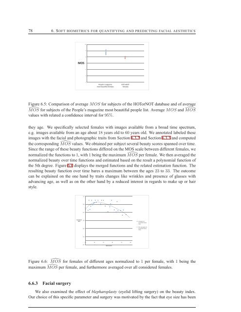
78 6. SOFT BIOMETRICS FOR QUANTIFYING AND PREDICTING FACIAL AESTHETICS Figure 6.5: Comparison of average MOS for subjects of the HOTorNOT database and of averagêMOS for subjects of the People’s magazine most beautiful people list. AverageMOS and ̂MOSvalues with related a confidence interval for 95%.they age. We specifically selected females with images available from a broad time spectrum,e.g. images available from an age about 18 years old to 60 years old. We annotated labeled theseimages with the facial and photographic traits from Section 6.3.2 and Section 6.3.3 and computedthe corresponding ̂MOS values. We obtained per subject several beauty scores spanned over time.Since the range of these beauty functions differed on the MOS scale between different females, wenormalized the functions to1, with1being the maximum ̂MOS per female. We then averaged thenormalized beauty over time functions and estimated based on the result a polynomial function ofthe 5th degree. Figure 6.6 displays the merged functions and the related estimation function. Theresulting beauty function over time bares a maximum between the ages 23 to 33. The outcomecan be explained on the one hand by traits changes like wrinkles and presence of glasses withadvancing age, as well as on the other hand by a reduced interest in regards to make up or hairstyle. Figure 6.6: ̂MOS for females of different ages normalized to 1 per female, with 1 being themaximum ̂MOS per female, and furthermore averaged over all considered females.6.6.3 Facial surgeryWe also examined the effect of blepharoplasty (eyelid lifting surgery) on the beauty index.Our choice of this specific parameter and surgery was motivated by the fact that eye size has been
79shown to have a high impact on our chosen beauty metric. We randomly selected 20 image pairs(before and after the surgery 2 , see Figure 6.7) from the plastic surgery database [SVB + 10], andafter annotation, we computed the related beauty indices. Interestingly our analysis suggested arelatively small surgery gain in the ̂MOS increase. Specifically the increase revealed a modestsurgery impact on the beauty index, with variations ranging in average between 1% and 4%.Figure 6.7: Examples of the Plastic Surgery Database. The left images depict the subjects beforesurgery, the right images after surgery.We proceed with the analysis and simulation of an automatic tool for facial beauty prediction.6.7 Towards an automatic tool for female beauty predictionAn automatic tool including classification regarding all 37 above presented traits will havethe benefit of a maximal achievable prediction score, at the same time though each automaticallydetected trait will bring an additional classification error into the prediction performance. Thus indesigning such an automatic tool a tradeoff between possible prediction score and categorizationerror has to be considered. We illustrate an analysis of prediction scores evoked by differentcombinations of traits in Table 6.2.Trait x iPearson’s correlationcoefficient r i,MOSx 1 0.5112x 1 , x 2 0.5921x 1 , x 2 , x 12 0.5923x 1 , x 2 , x 3 0.6319x 1 , x 2 , x 8 0.6165x 1 , x 2 , x 12 , x 15 0.5930x 1 , x 2 , x 3 , x 8 0.6502x 1 , x 2 , x 12 , x 15 , x 14 0.6070x 1 , x 2 , x 4 , x 12 , x 14 , x 15 0.6392x 1 , x 2 , x 4 , x 5 , x 12 , x 14 , x 15 0.6662x 1 , x 2 , x 4 , x 5 , x 12 , x 14 , x 15 , x 20 0.6711x 1 , x 2 , x 8 , x 14 , x 20 , x 23 0.6357Motivated by this Table 6.2 and towards simulating a realistic automatic tool for beauty prediction,we select a limited set of significant traits, x 1 ,x 2 ,x 8 , with other words factors describing1how big the eyes of a person 1 2 are, the ratio head width/head height and the presence of glasses.1 2 8Moreover we add acquisition traits with no extra error impact, such as x 14 ,x 20 ,x 23 , namely im-1 2 8 14 20 231age format, JPEG quality measure and image resolution. We then proceed to appropriate reliability1 21 2 8scores related tox 1 ,x 2 ,x 8 based on state of the art categorization algorithms:14 20 23 1 2 82. For this experiment all values attached to non permanent traits were artificially kept constant for "before surgery"and "after surgery" images.
- Page 29 and 30: 27In this setting we clearly assign
- Page 31 and 32: 29Table 3.1: SBSs with symmetric tr
- Page 33 and 34: 31corresponding to p(n,ρ). Towards
- Page 35 and 36: the same category (all subjects in
- Page 37 and 38: 3.5.2 Analysis of interference patt
- Page 39 and 40: an SBS by increasing ρ, then what
- Page 41 and 42: 39Table 3.4: Example for a heuristi
- Page 43 and 44: 41for a given randomly chosen authe
- Page 45 and 46: 43Chapter 4Search pruning in video
- Page 47 and 48: 45Figure 4.1: System overview.SBS m
- Page 49 and 50: 472.52rate of decay of P(τ)1.510.5
- Page 51 and 52: 49to be the probability that the al
- Page 53 and 54: 51The following lemma describes the
- Page 55 and 56: 534.5.1 Typical behavior: average g
- Page 57 and 58: 55n = 50 subjects, out of which we
- Page 59 and 60: 5710.950.9pruning Gain r(vt)0.850.8
- Page 61 and 62: 59for one person, for trait t, t =
- Page 63 and 64: 61Chapter 5Frontal-to-side person r
- Page 65 and 66: 63Figure 5.1: Frontal / gallery and
- Page 67 and 68: 6510.90.80.7Skin colorHair colorShi
- Page 69 and 70: 6710.90.80.70.6Perr0.50.40.30.20.10
- Page 71 and 72: 69Chapter 6Soft biometrics for quan
- Page 73 and 74: 71raphy considerations include [BSS
- Page 75 and 76: 73Figure 6.3: Example image of the
- Page 77 and 78: 75A direct way to find a relationsh
- Page 79: 77- Pearson’s correlation coeffic
- Page 83 and 84: 81Chapter 7Practical implementation
- Page 85 and 86: 834) Eye glasses detection: Towards
- Page 87 and 88: 857.2 Eye color as a soft biometric
- Page 89 and 90: 87Table 7.5: GMM eye color results
- Page 91 and 92: 89and office lights, daylight, flas
- Page 93 and 94: 917.5 SummaryThis chapter presented
- Page 95 and 96: 93Chapter 8User acceptance study re
- Page 97 and 98: 95Table 8.1: User experience on acc
- Page 99 and 100: 97scared of their PIN being spying.
- Page 101 and 102: 99Table 8.2: Comparison of existing
- Page 103 and 104: 101ConclusionsThis dissertation exp
- Page 105 and 106: 103Future WorkIt is becoming appare
- Page 107 and 108: 105Appendix AAppendix for Section 3
- Page 109 and 110: 107- We are now left withN −F = 2
- Page 111 and 112: 109Appendix BAppendix to Section 4B
- Page 113 and 114: 111Blue Green Brown BlackBlue 0.75
- Page 115 and 116: 113Appendix CAppendix for Section 6
- Page 117 and 118: 115Appendix DPublicationsThe featur
- Page 119 and 120: 117Bibliography[AAR04] S. Agarwal,
- Page 121 and 122: 119[FCB08] L. Franssen, J. E. Coppe
- Page 123 and 124: 121[Ley96] M. Leyton. The architect
- Page 125 and 126: 123[RN11] D. Reid and M. Nixon. Usi
- Page 127 and 128: 125[ZG09] X. Zhang and Y. Gao. Face
- Page 129: 2Rapporteurs:Prof. Dr. Abdenour HAD
78 6. <strong>SOFT</strong> <strong>BIOMETRICS</strong> FOR QUANTIFYING AND PREDICTING <strong>FACIAL</strong> AESTHETICS Figure 6.5: Comparison <strong>of</strong> average MOS for subjects <strong>of</strong> the HOTorNOT database and <strong>of</strong> averagêMOS for subjects <strong>of</strong> the People’s magazine most beautiful people list. AverageMOS and ̂MOSvalues with related a confidence interval for 95%.they age. We specifically selected females with images available from a broad time spectrum,e.g. images available from an age about 18 years old to 60 years old. We annotated labeled theseimages with the facial and photographic traits from Section 6.3.2 and Section 6.3.3 and computedthe corresponding ̂MOS values. We obtained per subject several beauty scores spanned over time.Since the range <strong>of</strong> these beauty functions differed on the MOS scale between different females, wenormalized the functions to1, with1being the maximum ̂MOS per female. We then averaged thenormalized beauty over time functions and estimated based on the result a polynomial function <strong>of</strong>the 5th degree. Figure 6.6 displays the merged functions and the related estimation function. Theresulting beauty function over time bares a maximum between the ages 23 to 33. The outcomecan be explained on the one hand by traits changes like wrinkles and presence <strong>of</strong> glasses withadvancing age, as well as on the other hand by a reduced interest in regards to make up or hairstyle. Figure 6.6: ̂MOS for females <strong>of</strong> different ages normalized to 1 per female, with 1 being themaximum ̂MOS per female, and furthermore averaged over all considered females.6.6.3 Facial surgeryWe also examined the effect <strong>of</strong> blepharoplasty (eyelid lifting surgery) on the beauty index.Our choice <strong>of</strong> this specific parameter and surgery was motivated by the fact that eye size has been


