Simulation of the Effects of an Air Blast Wave - ELSA - Europa
Simulation of the Effects of an Air Blast Wave - ELSA - Europa
Simulation of the Effects of an Air Blast Wave - ELSA - Europa
- No tags were found...

Create successful ePaper yourself
Turn your PDF publications into a flip-book with our unique Google optimized e-Paper software.
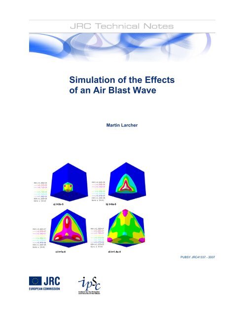
<strong>Simulation</strong> <strong>of</strong> <strong>the</strong> <strong>Effects</strong><strong>of</strong> <strong>an</strong> <strong>Air</strong> <strong>Blast</strong> <strong>Wave</strong>Martin Larchera) t=2e-5 b) t=6e-5c) t=1e-4 d) t=1.4e-4PUBSY JRC41337 - 2007
The Institute for <strong>the</strong> Protection <strong>an</strong>d Security <strong>of</strong> <strong>the</strong> Citizen provides researchbased, systemsorientedsupport to EU policies so as to protect <strong>the</strong> citizen against economic <strong>an</strong>d technologicalrisk. The Institute maintains <strong>an</strong>d develops its expertise <strong>an</strong>d networks in information,communication, space <strong>an</strong>d engineering technologies in support <strong>of</strong> its mission. The strongcrossfertilisation between its nuclear <strong>an</strong>d non-nuclear activities streng<strong>the</strong>ns <strong>the</strong> expertise it c<strong>an</strong>bring to <strong>the</strong> benefit <strong>of</strong> customers in both domains.Europe<strong>an</strong> CommissionJoint Research CentreInstitute for <strong>the</strong> Protection <strong>an</strong>d Security <strong>of</strong> <strong>the</strong> CitizenContact informationAddress: Martin Larcher, T.P. 480, Joint Research Centre, I-21020 Ispra, ITALYE-mail: martin.larcher@jrc.itTel.: +390332789004Fax: +390332789049http://ipsc.jrc.ec.europa.euhttp://www.jrc.ec.europa.euLegal NoticeNei<strong>the</strong>r <strong>the</strong> Europe<strong>an</strong> Commission nor <strong>an</strong>y person acting on behalf <strong>of</strong> <strong>the</strong> Commission isresponsible for <strong>the</strong> use which might be made <strong>of</strong> this publication.A great deal <strong>of</strong> additional information on <strong>the</strong> Europe<strong>an</strong> Union is available on <strong>the</strong> Internet.It c<strong>an</strong> be accessed through <strong>the</strong> <strong>Europa</strong> serverhttp://europa.eu/JRC 41337ISSN 1018-5593Luxembourg: Office for Official Publications <strong>of</strong> <strong>the</strong> Europe<strong>an</strong> Communities© Europe<strong>an</strong> Communities, 2007Reproduction is authorised provided <strong>the</strong> source is acknowledgedPrinted in Italy
Distribution ListLechner S.Anthoine A.Casadei F.Dyngel<strong>an</strong>d T.Géradin M.Gi<strong>an</strong>nopoulos G.Gutierrez E.Halleux J.P.Larcher M.Paffumi E. (JRC Petten)Pegon P.Solomos G.DG Tr<strong>an</strong>External:Mr. Bung H. (CEA)Faucher V. (CEA)Galon P. (CEA)Kill N. (Samtech)Cheruet A. (Samtech)Potapov S. (EDF)S. LechnerThe information contained in this document may not be disseminated,copied or utilized without <strong>the</strong> written authorization <strong>of</strong> <strong>the</strong> Commission.The Commission reserves specifically its rights to apply for patents orto obtain o<strong>the</strong>r protection for <strong>the</strong> matter open to intellectual or industrialprotection.
CONTENTS1 Introduction ...................................................................................................................................52 <strong>Air</strong> <strong>Blast</strong> <strong>Wave</strong>s.............................................................................................................................62.1 Introduction..........................................................................................................................62.1.1 Detonations ......................................................................................................................62.1.2 <strong>Air</strong> <strong>Blast</strong> <strong>Wave</strong>s ...............................................................................................................72.2 Literature Data .....................................................................................................................82.2.1 Pressure-Time Distribution ..............................................................................................82.2.2 Maximum / Minimum Pressure .....................................................................................102.2.3 Impulse...........................................................................................................................112.2.4 Negative Phase...............................................................................................................112.2.5 <strong>Wave</strong> Form Parameter ...................................................................................................132.2.6 Shock Front Velocity .....................................................................................................162.2.7 Specific Heat Ratio ........................................................................................................163 Numerical Loading <strong>of</strong> a Structure with <strong>Air</strong> <strong>Blast</strong> <strong>Wave</strong>s............................................................184 Investigations with Explosives as a Charge (Solid TNT) ...........................................................204.1 Modelling <strong>of</strong> <strong>the</strong> explosive ................................................................................................204.2 Behaviour in <strong>the</strong> Explosive ................................................................................................244.3 Cone with two Symmetry Axes .........................................................................................294.4 Cubic Charge with two Symmetry Axes............................................................................384.5 Spherical Charge with two Symmetry Axes ......................................................................424.6 Comparison between <strong>the</strong> Different Models .......................................................................464.6.1 Maximum Pressure.........................................................................................................464.6.2 Impulse...........................................................................................................................474.6.3 Arrival Time...................................................................................................................494.6.4 Positive Phase Duration .................................................................................................494.6.5 Comparison with results <strong>of</strong> o<strong>the</strong>r authors ......................................................................504.7 Influence <strong>of</strong> several parameters .........................................................................................504.7.1 Specific heat ratio (CON15) ..........................................................................................504.7.2 Values for γ, E 0, ρ .........................................................................................................514.7.3 Parameters for <strong>the</strong> explosive ..........................................................................................514.7.4 Burn mass fraction .........................................................................................................515 Bubble model...............................................................................................................................526 Control Volume...........................................................................................................................586.1 Flux between <strong>the</strong> CL3D <strong>an</strong>d <strong>the</strong> fluid element ..................................................................586.2 Several models ...................................................................................................................587 Implementation <strong>of</strong> <strong>an</strong> <strong>Air</strong> <strong>Blast</strong> Loading Function .....................................................................627.1 Motivation..........................................................................................................................627.2 Used Function ....................................................................................................................627.3 Implementation ..................................................................................................................627.4 Verification with Examples................................................................................................638 Mesh generation for LS-DYNA ..................................................................................................649 References ...................................................................................................................................6510 Apendix..................................................................................................................................6710.1 EUROPLEXUS Code ........................................................................................................6710.2 Miscell<strong>an</strong>eous code ............................................................................................................7110.3 Sample input files...............................................................................................................744
1 IntroductionThis work is being conducted in <strong>the</strong> framework <strong>of</strong> <strong>the</strong> project RAILPROTECT, which deals with<strong>the</strong> security <strong>an</strong>d safety <strong>of</strong> rail tr<strong>an</strong>sport against terrorist attacks. The bombing threat is onlyconsidered, <strong>an</strong>d focus is placed on predicting <strong>the</strong> effects <strong>of</strong> explosions in railway <strong>an</strong>d metro stations<strong>an</strong>d rolling stock <strong>an</strong>d on assessing <strong>the</strong> vulnerability <strong>of</strong> such structures.The project is based on numerical simulations, which are carried out with <strong>the</strong> explicit FiniteElement Code EUROPLEXUS that is written for <strong>the</strong> calculation <strong>of</strong> fast dynamic fluid-structureinteractions. This program has been developed in a collaboration <strong>of</strong> <strong>the</strong> French Commissariat àl'Energie Atomique (CEA Saclay) <strong>an</strong>d <strong>the</strong> Joint Research Centre <strong>of</strong> <strong>the</strong> Europe<strong>an</strong> Commission (JRCIspra).As <strong>the</strong> aim <strong>of</strong> this project is to calculate <strong>the</strong> behaviour <strong>of</strong> structures under a loading produced by airblast waves, <strong>an</strong> indispensable starting point in this study is <strong>the</strong> ability to simulate <strong>the</strong> generation <strong>of</strong>such waves from a given qu<strong>an</strong>tity <strong>of</strong> explosive, <strong>an</strong>d to follow <strong>the</strong>ir propagation through 3D spacesas <strong>the</strong>y finally impinge onto <strong>the</strong> structures under consideration.The results <strong>of</strong> such numerical tests <strong>of</strong> free air blasts are presented in this report <strong>an</strong>d are compared toexperimental data available in <strong>the</strong> literature. In <strong>the</strong> absence <strong>of</strong> such data <strong>the</strong> EUROPLEXUS resultsare compared to <strong>the</strong> results <strong>of</strong> o<strong>the</strong>r codes, in particular to LS-DYNA, which is run in collaborationwith <strong>the</strong> University <strong>of</strong> Karlsruhe. This <strong>an</strong>alysis is preceded by <strong>an</strong> exposition <strong>of</strong> some basic conceptson blast wave characteristics, explosives, <strong>an</strong>d a description <strong>of</strong> <strong>the</strong> equation <strong>of</strong> state adopted hereinfor <strong>the</strong> modelling <strong>of</strong> <strong>the</strong> detonation <strong>of</strong> a solid explosive.5
2 <strong>Air</strong> <strong>Blast</strong> <strong>Wave</strong>s2.1 Introduction2.1.1 DetonationsExplosions c<strong>an</strong> be distinguished in detonations <strong>an</strong>d deflagrations. The difference between detonations<strong>an</strong>d deflagrations is <strong>the</strong> velocity <strong>of</strong> <strong>the</strong> reaction zone in <strong>the</strong> explosive. Deflagrations have aslower reaction zone th<strong>an</strong> <strong>the</strong> sound speed. Examples for deflagrations are <strong>the</strong> burning <strong>of</strong> gas-airmixtures<strong>an</strong>d slow explosives like gun powder.Detonations have a faster reaction zone th<strong>an</strong> <strong>the</strong> sound speed. The most common explosives reactwith detonations.To compare different explosives <strong>the</strong> TNT equivalent c<strong>an</strong> be used. The TNT equivalent is a methodfor qu<strong>an</strong>tifying <strong>the</strong> energy released in <strong>the</strong> detonation <strong>of</strong> <strong>an</strong> explosive subst<strong>an</strong>ce, by comparing it tothat <strong>of</strong> <strong>an</strong> equal qu<strong>an</strong>tity <strong>of</strong> TNT. It is known that 1 kg TNT releases <strong>the</strong> energy <strong>of</strong> 4.520x10 6 J.The TNT equivalent is available for st<strong>an</strong>dard explosives <strong>an</strong>d for some <strong>of</strong> <strong>the</strong>m it is summarized inTable 1.Explosive Mass Specificenergy [kJ/kg]TNTEquivalentTNT 4520 1Torpex 7540 1.667Semtex 1A 4980 1.102C4 6057 1.34Table 1: TNT equivalent for different explosivesThe effects <strong>of</strong> <strong>an</strong> explosion c<strong>an</strong> be distinguished in three r<strong>an</strong>ges:• Contact detonation: The explosive is in contact with <strong>the</strong> loaded material. The load-time functiondepends on <strong>the</strong> loaded material, which, in most cases, is destroyed. Occurrences are <strong>the</strong> blasting<strong>of</strong> concrete (demolition etc.) or terrorist attacks where <strong>the</strong> explosive is located directly on <strong>the</strong>structure.• Near zone <strong>of</strong> <strong>the</strong> explosion: In most cases he material is also directly damaged like in <strong>the</strong>contact zone.6
• Far zone. The blast wave resulting from <strong>the</strong> detonation dominates <strong>the</strong> effects on hum<strong>an</strong>s <strong>an</strong>dstructures.The size <strong>of</strong> all <strong>the</strong>se zones depends on <strong>the</strong> qu<strong>an</strong>tity <strong>of</strong> <strong>the</strong> explosive charge.Additional parameters for a detonation, depending on <strong>the</strong> size <strong>of</strong> <strong>the</strong> explosive, c<strong>an</strong> be defined. Forexample, <strong>the</strong> radius in which debris from <strong>the</strong> explosion (not from <strong>the</strong> blast wave) are possible isgiven by Kinney [15] as13r = 45W(1)where, r is expressed in m <strong>an</strong>d W is <strong>the</strong> TNT equivalent <strong>of</strong> <strong>the</strong> explosive in kg.2.1.2 <strong>Air</strong> <strong>Blast</strong> <strong>Wave</strong>sThe pressure that arrives at a certain point depends on <strong>the</strong> dist<strong>an</strong>ce <strong>an</strong>d on <strong>the</strong> size <strong>of</strong> <strong>the</strong> explosive.ppmaxpmintp0t at d t nFigure 1: Pressure-time curve for a free air blast waveThe main characteristics <strong>of</strong> <strong>the</strong> development <strong>of</strong> this pressure wave are <strong>the</strong> following:- The arrival time t a <strong>of</strong> <strong>the</strong> shock wave to <strong>the</strong> point under consideration. This includes <strong>the</strong> time<strong>of</strong> <strong>the</strong> detonation wave to propagate through <strong>the</strong> explosive charge.- The peak overpressure p max . The pressure attains its maximum very fast (extremely shortrise-time), <strong>an</strong>d <strong>the</strong>n starts decreasing until it reaches <strong>the</strong> reference pressure p o (in most cases<strong>the</strong> normal atmospheric pressure).- The positive phase duration t d , which is <strong>the</strong> time for reaching <strong>the</strong> reference pressure. Afterthis point <strong>the</strong> pressure drops below <strong>the</strong> reference pressure until <strong>the</strong> maximum negative7
pressure p min . The duration <strong>of</strong> <strong>the</strong> negative phase is denoted as t n .- The incident overpressure impulse, which is <strong>the</strong> integral <strong>of</strong> <strong>the</strong> overpressure curve over <strong>the</strong>positive phase t d .The idealised (free air blast) form <strong>of</strong> <strong>the</strong> pressure wave <strong>of</strong> Figure 1 c<strong>an</strong> be greatly altered by <strong>the</strong>morphology <strong>of</strong> <strong>the</strong> medium encountered along its propagation. For inst<strong>an</strong>ce, peak pressure c<strong>an</strong> beincreased up to 8 times if <strong>the</strong> wave is reflected on a rigid obstacle. The effects <strong>of</strong> <strong>the</strong> reflectiondepend on <strong>the</strong> geometry, <strong>the</strong> size <strong>an</strong>d <strong>the</strong> <strong>an</strong>gle <strong>of</strong> incidence. By setting γ = 1.4 (ratio <strong>of</strong> specificheats <strong>of</strong> air), it c<strong>an</strong> be shown that <strong>the</strong> reflected overpressure p r ispr2 p⎡7p+ 4p0 max=max ⎢ ⎥7 p0 + pmax⎣⎤⎦(2)All parameters <strong>of</strong> <strong>the</strong> pressure time curve are normally written in terms <strong>of</strong> a scaled dist<strong>an</strong>ceZ = d3W(3)where W is <strong>the</strong> mass <strong>of</strong> <strong>the</strong> explosive charge <strong>an</strong>d d <strong>the</strong> dist<strong>an</strong>ce to <strong>the</strong> centre <strong>of</strong> <strong>the</strong> charge.2.2 Literature Data2.2.1 Pressure-Time DistributionThere are available in <strong>the</strong> literature several pressure-time-curves for different kinds <strong>of</strong> explosions.The effects <strong>of</strong> nuclear explosions here should be disregarded.The pressure at a known point c<strong>an</strong> be described by <strong>the</strong> modified Friedl<strong>an</strong>der equation (from Baker[2]) <strong>an</strong>d depends on <strong>the</strong> time t from <strong>the</strong> arrival <strong>of</strong> <strong>the</strong> pressure wave at this point ( t = t0−t a)⎛ t ⎞pt () = p0 + pmax⎜1−⎟⎝ td⎠bt−td(4)The o<strong>the</strong>r parameters involved are <strong>the</strong> atmospheric pressure p 0 , <strong>the</strong> maximum overpressure p max <strong>an</strong>d<strong>the</strong> duration <strong>of</strong> <strong>the</strong> positive pressure t d . The parameter b describes <strong>the</strong> decay <strong>of</strong> <strong>the</strong> curve. It c<strong>an</strong> becalculated with a known minimum pressure after <strong>the</strong> positive phase. Alternatively, <strong>the</strong> parameter bc<strong>an</strong> be calculated with <strong>the</strong> knowledge <strong>of</strong> <strong>the</strong> impulse. This will be done in chapter 2.2.5.All parameters for <strong>the</strong> pressure-time curve c<strong>an</strong> be taken from different diagrams <strong>an</strong>d equations(Baker [2], Kinney [15], Kingery [14], see e.g. Figure 2).8
Figure 2: Model <strong>of</strong> Kingery [14] with scaled dist<strong>an</strong>ces9
2.2.2 Maximum / Minimum PressureKingery [14] developed in 1984 curves for <strong>the</strong> description <strong>of</strong> <strong>the</strong> different air blast parameters byusing a rich body <strong>of</strong> experimental data, which had been properly homogenised. The parameters arepresented in double logarithmic diagrams with <strong>the</strong> scaled dist<strong>an</strong>ce Z as abscissa, but are alsoavailable as polynomial equations. These diagrams <strong>an</strong>d equations enjoy <strong>the</strong> greatest overallaccept<strong>an</strong>ce <strong>an</strong>d are widely used as reference by most researchers. The parameters are alsoimplemented in different computer programs that c<strong>an</strong> be used for <strong>the</strong> calculation <strong>of</strong> air blast wavevalues. e.g. <strong>the</strong>y are implemented in ConWep – a program developed from <strong>the</strong> US-Army thatcalculates conventional weapons effects. The same curves are also used for <strong>an</strong> easy air blast loadmodel (*LOAD_BLAST) in LS-DYNA. Also in [14] curves are provided for reflection effects(surface burst <strong>of</strong> hemispherical charges) <strong>an</strong>d free air conditions (spherical charge).Ano<strong>the</strong>r equation has been proposed by Kinney [15], in which <strong>the</strong> overpressure-dist<strong>an</strong>ce relation forchemical explosions c<strong>an</strong> be written asp=2⎡ ⎛ Z ⎞ ⎤808⎢1+ ⎜ ⎟ ⎥⎢⎣⎝4.5⎠ ⎥⎦maxp0Z2Z2Z2⎛ ⎞ ⎛ ⎞ ⎛ ⎞1+ ⎜ ⎟ 1+ ⎜ ⎟ 1+⎜ ⎟⎝0.048 ⎠ ⎝0.32 ⎠ ⎝1.35⎠(5)Figure 3 shows <strong>the</strong> small differences between <strong>the</strong> two models.Figure 3: Difference <strong>of</strong> <strong>the</strong> model <strong>of</strong> Kingery <strong>an</strong>d <strong>the</strong> model <strong>of</strong> Kinney with 1kg TNT10
2.2.3 ImpulseThe impulse <strong>of</strong> <strong>the</strong> air blast wave has a big influence on <strong>the</strong> response <strong>of</strong> <strong>the</strong> structures. The impulseis defined here as <strong>the</strong> area under <strong>the</strong> pressure time curve with <strong>the</strong> unit <strong>of</strong> pressure*sec. The impulsec<strong>an</strong> be calculated with (Kinney [15])0.067 1 + ( Z / 0.23)I =2 34Z 1 + ( Z /1.55)4(6)Ano<strong>the</strong>r possibility is <strong>the</strong> polynomial equation <strong>of</strong> Kingery [14]. The comparison <strong>of</strong> <strong>the</strong> impulseresulting from both equations shows that <strong>the</strong> equation <strong>of</strong> Kinney simplifies <strong>the</strong> curve <strong>of</strong> <strong>the</strong> impulsebetween a scaled dist<strong>an</strong>ce <strong>of</strong> 0.5 <strong>an</strong>d 1.5 m/kg 1/3 .800600impulse [Pa sec]400200KinneyKingery00 0.5 1 1.5 2 2.5 3scaled dist<strong>an</strong>ce [m/kg 1/3 ]Figure 4: Different equations for <strong>the</strong> impulse (Kinney [15] <strong>an</strong>d Kingery [14])2.2.4 Negative PhaseDetonations produce <strong>an</strong> overpressure peak, <strong>an</strong>d afterwards <strong>the</strong> pressure decreases <strong>an</strong>d drops below<strong>the</strong> reference pressure (generally <strong>the</strong> atmospheric pressure). The influence <strong>of</strong> <strong>the</strong> so-called negativephase depends on <strong>the</strong> scaled dist<strong>an</strong>ce. For scaled dist<strong>an</strong>ces Z larger th<strong>an</strong> 20 <strong>an</strong>d especially for Zlarger th<strong>an</strong> 50 <strong>the</strong> influence <strong>of</strong> <strong>the</strong> negative phase c<strong>an</strong> not always be neglected. The size <strong>of</strong> <strong>the</strong>positive impulse <strong>an</strong>d <strong>of</strong> <strong>the</strong> negative impulse is <strong>the</strong>n nearly <strong>the</strong> same. If <strong>the</strong> structure c<strong>an</strong> react11
successfully to <strong>the</strong> positive pressure but is more sensitive to a negative pressure, failure <strong>of</strong> parts <strong>of</strong><strong>the</strong> structure c<strong>an</strong> result from this negative pressure phase (see Krauthammer [16]). However, inseveral cases <strong>the</strong> negative phase is neglected e.g. in <strong>the</strong> air blast function <strong>of</strong> <strong>the</strong> CONWEP-Code.Smith [22] presents <strong>the</strong> following equation to calculate <strong>the</strong> value <strong>of</strong> <strong>the</strong> negative pressurepmin0.35 105 Pa for Z 1.6= > (7)ZThe duration time <strong>of</strong> <strong>the</strong> negative pressuretnpminc<strong>an</strong> be calculated with1/3= 0.00125 W [sec](8)Ano<strong>the</strong>r possibility to get <strong>the</strong>se parameters is a diagram (see Figure 5) in Krauthammer [16]. Byusing this diagram <strong>the</strong> limitation <strong>of</strong> equation (7) c<strong>an</strong> be overcome by assumingppminmin0.35 105 Pa for Z 3.5=Z>=
Figure 5: Different parameters for <strong>the</strong> negative phase (see Krauthammer [16])2.2.5 <strong>Wave</strong> Form ParameterThe decay or form parameter b in <strong>the</strong> Friedl<strong>an</strong>der equation (4) describes <strong>the</strong> decay <strong>of</strong> <strong>the</strong> pressuretimecurve. The Friedl<strong>an</strong>der equation has <strong>the</strong> parameters p max , t d <strong>an</strong>d b. p max <strong>an</strong>d t d c<strong>an</strong> be readilyfound as explained before. There are several possibilities to calculate <strong>the</strong> decay parameter b byusing <strong>an</strong>o<strong>the</strong>r known value <strong>of</strong> <strong>the</strong> pressure-time curve:1. Using <strong>the</strong> minimal pressure in <strong>the</strong> negative phase. Then, as it will be shown, <strong>the</strong> impulse <strong>of</strong><strong>the</strong> positive phase is not accurate.2. Using <strong>the</strong> impulse <strong>of</strong> <strong>the</strong> positive phase. Then, as it will be shown, <strong>the</strong> minimal pressure in<strong>the</strong> negative phase is not accurate. An additional equation for <strong>the</strong> negative phase should beused to avoid a smaller underpressure th<strong>an</strong> <strong>the</strong> atmospheric pressure.Kinney [14] <strong>an</strong>d Baker [3] calculate <strong>the</strong> parameter b by using <strong>the</strong> impulse <strong>of</strong> <strong>the</strong> positive phase.They use different equations for <strong>the</strong> pressure, for <strong>the</strong> impulse <strong>an</strong>d for <strong>the</strong> duration <strong>of</strong> <strong>the</strong> positivephase. Therefore, <strong>the</strong> results for <strong>the</strong> parameter b differ (see Figure 6).Both methods, described above, for <strong>the</strong> calculation <strong>of</strong> <strong>the</strong> decay parameter b should be used here tosee <strong>the</strong> difference between <strong>the</strong> results. The Friedl<strong>an</strong>der equation is too complex to solve13
<strong>an</strong>alytically, <strong>an</strong>d a program written in C++ c<strong>an</strong> be used for <strong>the</strong> approximation. The listing is shownin <strong>the</strong> appendix.At <strong>the</strong> first step <strong>the</strong> negative pressure with <strong>the</strong> values from Kingery are used. The results for b differfrom <strong>the</strong> function <strong>of</strong> Kinney [13] <strong>an</strong>d Baker [3] (see Figure 6). The comparison <strong>of</strong> <strong>the</strong> resultedimpulses (see Figure 7) shows that <strong>the</strong> parameter b calculated with <strong>the</strong> minimal pressure in <strong>the</strong>negative phase gets a too small positive impulse <strong>an</strong>d should not be used.108KinneyBakerb [-]64Parameter b by using pminParameter b by using <strong>the</strong>impulse <strong>of</strong> <strong>the</strong> postive phase200 5 10 15 20 25 30 35 40Z [m/kg 1/3 ]Figure 6: Decay parameter b – different methods14
250200Impulse from KingeryImpulse with b from KinneyImpulse with b from BakerImpulse with b by using pminImpulse [Pa sec]1501005000 2 4 6 8 10 12 14 16 18 20Scaled dist<strong>an</strong>ce Z [m/kg 1/3 ]Figure 7: Decay parameter b – resulting impulse in comparison with <strong>the</strong> impulse from KingeryTherefore, <strong>the</strong> parameter b is next calculated using <strong>the</strong> impulse <strong>of</strong> <strong>the</strong> positive phase. Then, <strong>the</strong>resulting curve <strong>of</strong> b is similar to <strong>the</strong> curves <strong>of</strong> Kinney <strong>an</strong>d Baker. The exponential trend line givenby Excel has <strong>the</strong> following equationb1.1975= 5.2777⋅ Z −(11)The pressure time curve that is built with this b doesn’t fulfil <strong>the</strong> minimal pressure in <strong>the</strong> negativephase. Sometimes <strong>the</strong> pressure p is smaller th<strong>an</strong> <strong>the</strong> atmospheric pressure. This results in <strong>an</strong>impossible state <strong>of</strong> <strong>the</strong> air. Therefore, <strong>the</strong> approximation <strong>of</strong> <strong>the</strong> negative phase is done with abilinear curve shown in equation (12) <strong>an</strong>d Figure 8 by using <strong>the</strong> values <strong>of</strong> <strong>the</strong> negative phase shownin section 2.2.4.⎛tt ⎞ dp= p0 + pmax⎜1 − ⎟ for t < td⎝ td⎠2 pntnp= p0− ( t− td) for t > td ∧ t < td+t22 pntnp = p0− ( t + t − t) for t > t + ∧ t < t + tt2p= p for t > t + t0nnbt−d n d d ndn(12)15
Figure 8: Pressure-time curve for a free air blast wave – approximation <strong>of</strong> <strong>the</strong> negative phase2.2.6 Shock Front VelocityThe arrival time <strong>of</strong> <strong>the</strong> shock front at different points c<strong>an</strong> be used to calculate <strong>the</strong> velocity <strong>of</strong> <strong>the</strong>shock front. With <strong>the</strong> knowledge <strong>of</strong> this velocity <strong>the</strong> pressure c<strong>an</strong> be obtained with <strong>the</strong> R<strong>an</strong>kine-Hugoniot relationship.Kingery [14] calculates also <strong>the</strong> shock front velocity depending on <strong>the</strong> pressure as⎛ γ + 1 pu = c0⎜1+⎝ 2γpmax0⎞⎟⎠1/2(13)The parameter γ (ratio <strong>of</strong> specific heats <strong>of</strong> air) depends also on <strong>the</strong> overpressure <strong>an</strong>d c<strong>an</strong> be takenfrom a table in [13]; c 0is <strong>the</strong> sound velocity in air (331 m/sec);p0is <strong>the</strong> atmospheric pressure (101.3 kPa).2.2.7 Specific Heat RatioThe specific heat ratio γ is defined asccpmaxis <strong>the</strong> peak overpressure <strong>an</strong>dpγ = (14)with c p being <strong>the</strong> specific heat at const<strong>an</strong>t pressure <strong>an</strong>d c v <strong>the</strong> specific heat at const<strong>an</strong>t volume. Bothv16
<strong>the</strong> specific heat ratio <strong>an</strong>d <strong>the</strong> speed <strong>of</strong> sound depend on <strong>the</strong> temperature, <strong>the</strong> pressure, <strong>the</strong> humidity,<strong>an</strong>d <strong>the</strong> CO 2 concentration. Kingery [14] defines <strong>the</strong> variation <strong>of</strong> <strong>the</strong> specific heat ratio with a r<strong>an</strong>ge<strong>of</strong> 1.402 to 1.176.17
3 Numerical Loading <strong>of</strong> a Structure with <strong>Air</strong> <strong>Blast</strong> <strong>Wave</strong>sThere are several ways <strong>of</strong> numerical modelling in order to load a structure with <strong>an</strong> air blast wave.These methods differ in <strong>the</strong> number <strong>of</strong> used elements <strong>an</strong>d with <strong>the</strong>m in <strong>the</strong> calculation time.• Model with <strong>the</strong> mech<strong>an</strong>ical modelling <strong>of</strong> <strong>the</strong> explosive (JWL-equation (15)). A fine mesh isessential to get realistic results. The size <strong>of</strong> <strong>the</strong> element in <strong>the</strong> r<strong>an</strong>ge around <strong>the</strong> explosive shouldbe approximately 1 mm. These calculations are very expensive. To reduce <strong>the</strong> computation timepartitioning c<strong>an</strong> be used. This method reduces <strong>the</strong> calculation time for models with a largevariation <strong>of</strong> element sizes.• The method proposed by Clutter [9] is also a solid TNT model <strong>an</strong>d uses only one element for<strong>the</strong> explosive. This is possible by different not specified methods in combination with <strong>the</strong>Becker-Kistiakowsky-Wilson EOS for <strong>the</strong> explosive.• 1D to 3D. This modelling is proposed in [4] <strong>an</strong>d is also a solid TNT model. A 1D calculation isused until <strong>the</strong> wave reaches a surface. Then <strong>the</strong> values <strong>of</strong> <strong>the</strong> density, energy, velocity <strong>an</strong>dpressure are mapped into <strong>the</strong> 3D mesh. Rose [20] maps <strong>the</strong> 1D model to 2D when <strong>the</strong> wavearrives <strong>the</strong> first surface <strong>an</strong>d maps <strong>the</strong> 2D model to 3D when <strong>the</strong> wave arrives a second surfacewith <strong>an</strong>o<strong>the</strong>r direction. EUROPLEXUS allows <strong>the</strong> implementation <strong>of</strong> this method. The methodshould also be validated with a calculation <strong>of</strong> <strong>the</strong> first model. The model is a mixture <strong>of</strong> <strong>the</strong> first<strong>an</strong>d <strong>the</strong> third model. The calculation time should be larger th<strong>an</strong> for <strong>the</strong> second model.• Model with a compressed bubble. The pressure-time function resulting from a compressedbubble c<strong>an</strong> not easily match <strong>the</strong> curve <strong>of</strong> <strong>an</strong> air blast wave. The size <strong>of</strong> <strong>the</strong> compression c<strong>an</strong> becalibrated with <strong>the</strong> maximum pressure or <strong>the</strong> impulse. The calculation time is smaller th<strong>an</strong> for<strong>the</strong> first model.• Control volume. A volume around <strong>the</strong> explosive is loaded by a pressure-time curve. Thispressure time curve c<strong>an</strong> be calculated with a model based on <strong>the</strong> modelling <strong>of</strong> <strong>the</strong> explosive.Alternatively, <strong>the</strong> well known curves from Kingery [14] c<strong>an</strong> be used. This method should bevalidated through comparisons with calculations <strong>of</strong> <strong>the</strong> first model. The computation time is in<strong>the</strong> r<strong>an</strong>ge <strong>of</strong> <strong>the</strong> second model.• Load-time function. This is only usable for <strong>an</strong> estimation <strong>of</strong> <strong>the</strong> behaviour <strong>of</strong> a structure loadedby <strong>an</strong> air blast wave. The structure is loaded by a load-time function built with <strong>the</strong> pressure-timefunction e.g. from Kingery [14]. This function is implemented in EUROPLEXUS (see chapter7). The calculation is relatively inexpensive. Alternatively, <strong>the</strong> pressure-time function c<strong>an</strong> be18
determined with a fluid pre-calculation with fixed boundaries for <strong>the</strong> structure. The structure is<strong>the</strong>n loaded by <strong>the</strong> pressures resulting from this fluid calculation.The choice among <strong>the</strong>se methods depends on <strong>the</strong> scope <strong>of</strong> <strong>the</strong> <strong>an</strong>alysis <strong>an</strong>d on fur<strong>the</strong>r investigationsabout <strong>the</strong>ir adv<strong>an</strong>tages <strong>an</strong>d shortcomings. Figure 9 shows different models for <strong>the</strong> simulation <strong>of</strong> <strong>an</strong>air blast wave.Solid TNTCompressed bubbleLoad on a control volumeLoad-time functionFigure 9: Several models for air blast wave simulations19
4 Investigations with Explosives as a Charge (Solid TNT)The aim <strong>of</strong> <strong>the</strong> RAILPROTECT project is to contribute to alleviating <strong>the</strong> vulnerability <strong>of</strong> Europe'spassenger tr<strong>an</strong>sport infrastructures. The effects <strong>of</strong> a terrorist attack should be simulated numerically,<strong>an</strong>d for a numerical investigation <strong>the</strong> knowledge <strong>of</strong> <strong>the</strong> loading <strong>of</strong> <strong>the</strong> structures is necessary. Thereare different approaches <strong>an</strong>d possibilities for <strong>the</strong> calculation <strong>of</strong> a detonation inside buildings, asdiscussed in chapter 3.A detonation releases a large amount <strong>of</strong> energy in a very short time. This results in <strong>an</strong> air shockwavewhich is spread outwards from <strong>the</strong> charge. Then, <strong>the</strong> air blast wave reaches <strong>the</strong> structure,which, depending on <strong>the</strong> size <strong>of</strong> <strong>the</strong> charge <strong>an</strong>d on <strong>the</strong> dist<strong>an</strong>ce, will respond to this wave loading.A calculation <strong>of</strong> <strong>the</strong> behaviour <strong>of</strong> <strong>the</strong> air blast wave requires <strong>the</strong> knowledge <strong>of</strong> <strong>the</strong> behaviour <strong>of</strong> <strong>the</strong>explosive <strong>an</strong>d <strong>of</strong> <strong>the</strong> air around <strong>the</strong> explosive. The results <strong>of</strong> <strong>the</strong> numerical investigation c<strong>an</strong> becompared for <strong>the</strong> validity <strong>of</strong> <strong>the</strong> calculations with existing experimental-<strong>an</strong>alytical data. As will beshown in this chapter, <strong>the</strong> experimental-<strong>an</strong>alytical results <strong>of</strong> Kingery [14] will constitute <strong>the</strong> basisfor <strong>the</strong>se comparisons.4.1 Modelling <strong>of</strong> <strong>the</strong> explosiveThe explosive for <strong>the</strong> numerical investigation c<strong>an</strong> be built up e.g. with <strong>the</strong> Jones–Wilkins–Lee(JWL)-equation. This equation <strong>of</strong> state (EOS) is widely used because <strong>of</strong> its simplicity <strong>an</strong>d due to <strong>the</strong>fact that most high explosives are well modelled by this equation. According to it, <strong>the</strong> value <strong>of</strong>pressure is given as⎛ ω ⎞−RV⎛ ω ⎞1 −R2VEpEOS= A⎜1− ⎟e + B⎜1− ⎟e+ ω⎝ RV1 ⎠ ⎝ RV2 ⎠ V(15)In this equation A, B, R1, R2 <strong>an</strong>d ω are <strong>the</strong> model parameters, V is <strong>the</strong> ratio ρ sol /ρ, where ρ=currentdensity <strong>an</strong>d ρ sol =density <strong>of</strong> solid explosive, <strong>an</strong>d E is <strong>the</strong> internal energy per unit volume <strong>of</strong> <strong>the</strong>explosive. It is noted that E=ρ sol e int , where e int is <strong>the</strong> current internal energy per unit mass. Theparameters <strong>of</strong> this equation for most explosives are shown in Dobratz [10]. Different authors useslightly differing parameter values for this equation, as shown in Table 2. Note that <strong>the</strong> equationwill be reduced only to its last term if <strong>the</strong> solid explosive is exhausted <strong>an</strong>d <strong>the</strong> resulting gases fullyexp<strong>an</strong>ded. The last term <strong>of</strong> equation (15) is <strong>the</strong> EOS <strong>of</strong> <strong>an</strong> ideal gas that c<strong>an</strong> be used e.g. for <strong>the</strong> air.pEOSE= ω (16)V20
From this asymptotic form it c<strong>an</strong> also be concluded that ω=γ-1 (γ=ratio <strong>of</strong> specific heats).Parameter Description ref.[6] AUTODYN ref.[21]- m<strong>an</strong>ualparameters usedfor <strong>the</strong> airA (Pa) 3.738e11 3.7377e11 3.712e11B (Pa) 3.747e9 3.7471e9 3.21e9R1 4.15 4.15 4.15R2 0.90 0.90 0.95ρ sol (kg/m3) density 1630 1630 1630 1.3e int (J/kg) current internal 3.68e6 3.68e6 4.29e6 2.1978E5energy per unit massγ specific heat ratio 1.35 1.35 1.30 1.30v det (m/sec) detonation speed 6930 6930 6930Table 2: Parameters for <strong>the</strong> JWL equation for TNTFor <strong>the</strong> air <strong>the</strong> same EOS will be used without a detonation <strong>an</strong>d different starting density <strong>an</strong>dinternal energy. By ignoring <strong>the</strong> explosion, <strong>the</strong> last part <strong>of</strong> <strong>the</strong> JWL-equation will prevail <strong>an</strong>d<strong>the</strong>refore, <strong>an</strong> ideal gas will be used.Different FE-Codes smear <strong>the</strong> detonation front over different time steps. This procedure is calledburn fraction <strong>an</strong>d its motivation is to control <strong>the</strong> release <strong>of</strong> <strong>the</strong> chemical energy for <strong>the</strong> simulation.The effects <strong>of</strong> <strong>the</strong> combustion on <strong>the</strong> pressure c<strong>an</strong> be considered with this formula( ( 1 2))p = p min 1, max F,F(17)The burn mass functions F 1 <strong>an</strong>d F 2 are computed by (see LS-DYNA <strong>an</strong>d [18])EOS( )⎧2t−t1 d⋅Ae,max⎪if t > t1F1= ⎨ 3νe⎪⎩ 0 if t ≤ t1(18)1−VF2= (19)− V1CJwhere t 1 is <strong>the</strong> ignition time <strong>of</strong> <strong>the</strong> observed element (calculated with <strong>the</strong> detonation velocity d),A e,max is <strong>the</strong> maximum surface area <strong>an</strong>d ν e <strong>the</strong> volume <strong>of</strong> <strong>the</strong> element. V is <strong>the</strong> actual specificvolume <strong>an</strong>d V CJ <strong>the</strong> specific volume at <strong>the</strong> Chapm<strong>an</strong>-Jouguet-pressure. The Chapm<strong>an</strong>-Jouguet21
pressure is reached if <strong>the</strong> sonic velocity <strong>of</strong> <strong>the</strong> reaction gases reaches <strong>the</strong> detonation velocity. Thevolume at <strong>the</strong> Chapm<strong>an</strong>-Jouguet-point isVCJ= − P(20)CJ12ρ0dThe term F 1 <strong>of</strong> <strong>the</strong> burn mass function intends to spread <strong>the</strong> burn front over several elements. Thesecond term should control <strong>the</strong> releasing <strong>of</strong> <strong>the</strong> energy. Interestingly, MSC-Dytr<strong>an</strong> uses only <strong>the</strong>term (19), whereas ABAQUS uses only one burn mass function( − )⎧ t t1d⎪ if t > t1Fb = ⎨ BS ⋅le⎪⎩ 0 if t ≤ t1(21)In this formula B S is <strong>the</strong> const<strong>an</strong>t that controls <strong>the</strong> width <strong>of</strong> <strong>the</strong> burn wave (set to a value <strong>of</strong> 2.5) <strong>an</strong>dl e is <strong>the</strong> element length. This function is very similar to (18).A 3D model <strong>of</strong> explosive is used to show <strong>the</strong> influence <strong>of</strong> <strong>the</strong> different burn mass fractions (Figure12, explosive4), whose different components c<strong>an</strong> be compared in Figure 10 <strong>an</strong>d Figure 11. Theinfluence <strong>of</strong> <strong>the</strong> term (21) is visible. The slope <strong>of</strong> <strong>the</strong> pressure peak decreases with F b , <strong>an</strong>d <strong>the</strong>arrival <strong>of</strong> <strong>the</strong> pressure peak is later. The calculations with EUROPLEXUS do not show <strong>an</strong> influence<strong>of</strong> <strong>the</strong> second term (F 2 ). Both curves are almost identical.LS-DYNA uses <strong>the</strong> functions (18) <strong>an</strong>d (19) for calculations with <strong>the</strong>MAT_HIGH_EXPLOSIVE_BURN model. The input syntax allows calculations with bothfunctions (beta=0) or only with <strong>the</strong> function (19) (beta=1). The model in LS-DYNA was built withhexahedral with <strong>an</strong> element size <strong>of</strong> 0.001 m. The results <strong>of</strong> a 3D model show that <strong>the</strong> burn massfraction in LS-DYNA reduces also <strong>the</strong> slope <strong>of</strong> <strong>the</strong> pressure peak. Never<strong>the</strong>less, <strong>the</strong> differencebetween <strong>the</strong> calculations with beta=0 <strong>an</strong>d beta=1 is negligible. The differences <strong>of</strong> <strong>the</strong> calculationsbetween EUROPLEXUS <strong>an</strong>d LS-DYNA are <strong>the</strong> smaller peak in LS-DYNA <strong>an</strong>d <strong>the</strong> higher pressurevalues behind <strong>the</strong> peak (here for a dist<strong>an</strong>ce less th<strong>an</strong> 0.04 m). The impulses are nearly <strong>the</strong> same (LS-DYNA 2.07 10 8 Pa sec, EUROPLEXUS 2.00 10 8 Pa sec).Therefore, <strong>the</strong> burn mass fraction is for <strong>the</strong> future work implemented only with <strong>the</strong> equation (21).22
2.0E+101.6E+10without burn mass fractionburn mass fraction Fbburn mass fraction Fb <strong>an</strong>d F2LS-DYNA beta=0LS-DYNA beta=1Pressure [Pa]1.2E+108.0E+094.0E+090.0E+000 0.01 0.02 0.03 0.04 0.05 0.06Dist<strong>an</strong>ce [m]Figure 10: Influence <strong>of</strong> <strong>the</strong> burn mass fraction in EUROPLEXUS (t=7 10 -6 sec)2.0E+101.6E+10EUROPLEXUS bmf=0EUROPLEXUS bmf=2.5LS-DYNA beta=0LS-DYNA beta=1Pressure [Pa]1.2E+108.0E+094.0E+090.0E+000.04 0.05 0.06 0.07 0.08 0.09 0.1Dist<strong>an</strong>ce [m]Figure 11: Influence <strong>of</strong> <strong>the</strong> burn mass fraction in EUROPLEXUS (t=1.4 10 -5 sec)Ano<strong>the</strong>r EOS for explosive is <strong>the</strong> “Ignition <strong>an</strong>d Growth Reactive Model” based on Tarver et al.[23]. This model c<strong>an</strong> also be used for <strong>the</strong> burning <strong>of</strong> propell<strong>an</strong>t (deflagrations).23
4.2 Behaviour in <strong>the</strong> ExplosiveThe blast behaviour in <strong>the</strong> air is affected by <strong>the</strong> development <strong>of</strong> <strong>the</strong> pressure in <strong>the</strong> explosive.Therefore, it should be investigated, whe<strong>the</strong>r <strong>the</strong> numerical simulation c<strong>an</strong> sufficiently represent <strong>the</strong>behaviour <strong>of</strong> <strong>the</strong> explosive.The numerical model for <strong>the</strong> explosive calculates <strong>the</strong> pressure with <strong>the</strong> JWL-equation (15). Anaccurate model for <strong>the</strong> development <strong>of</strong> <strong>the</strong> detonation front is used (See [1]). The detonation startsat <strong>the</strong> initiation point, <strong>an</strong>d <strong>the</strong> detonation front is moved with <strong>the</strong> given velocity <strong>of</strong> <strong>the</strong> detonation.An element detonates if <strong>the</strong> detonation front reaches this element. From this time <strong>the</strong> JWL-equationwill be used for this element.A spherical TNT charge <strong>of</strong> volume <strong>of</strong> 8000 cm 3 , i.e. with a radius <strong>of</strong> 0.124 m is considered. Tocontrol <strong>the</strong> behaviour <strong>of</strong> <strong>the</strong> pressure in <strong>the</strong> explosive a conical model is used (similar to <strong>the</strong> model<strong>of</strong> chapter 4.3, see Figure 12).lengthxopeningd pyrad ex,ind ex,endFigure 12: 3D simplified model for <strong>the</strong> behaviour in <strong>the</strong> explosiveThe models use hexahedrons <strong>an</strong>d a pyramid for <strong>the</strong> top <strong>of</strong> <strong>the</strong> model. The FSR-condition is used forall surfaces <strong>of</strong> <strong>the</strong> model. The difference between <strong>the</strong> meshes, listed in Table 3, is <strong>the</strong> refinement.24
Case opening d pyra d ex,in d ex,end Number <strong>of</strong> elementsexplosive1 Euleri<strong>an</strong> 2e-2 0.001 0.001 0.01 33explosive2 Euleri<strong>an</strong> 1e-2 0.0005 0.0005 0.005 65explosive3 Euleri<strong>an</strong> 4e-3 0.0005 0.0002 0.002 159explosive4 Euleri<strong>an</strong> 2e-3 0.0002 0.0001 0.001 318explosive5 Euleri<strong>an</strong> 2e-3 0.0002 0.0001 0.0005 499explosive6 Euleri<strong>an</strong> 2e-3 0.0002 0.0001 0.0002 859explosive7 ALE 2e-3 0.0002 0.0001 0.0005 499Table 3: Comparison <strong>of</strong> different models for <strong>the</strong> explosiveThe pressures are here <strong>an</strong>alysed in intervals <strong>of</strong> 1µsec. The procedure to get <strong>the</strong> values in space(SCOURBE comm<strong>an</strong>d in EUROPLEXUS) uses <strong>the</strong> averaged elemental pressure values for <strong>the</strong>nodal values. This results in a half value <strong>of</strong> <strong>the</strong> pressure at <strong>the</strong> node between <strong>an</strong> element inside <strong>an</strong>d<strong>an</strong> element outside <strong>of</strong> <strong>the</strong> detonation zone (see Figure 13). The vertical lines in this figurecorrespond to <strong>the</strong> dist<strong>an</strong>ces <strong>of</strong> <strong>the</strong> elements that are detonated at a certain time step (c<strong>an</strong> be get from<strong>the</strong> listing). The detonation front c<strong>an</strong> be identified by <strong>the</strong> steep increasing <strong>of</strong> <strong>the</strong> pressure.Therefore, it is import<strong>an</strong>t to consider <strong>the</strong> value <strong>of</strong> <strong>the</strong> last element <strong>of</strong> <strong>the</strong> detonation front <strong>an</strong>d not <strong>the</strong>value <strong>of</strong> <strong>the</strong> last node.Figure 13: Distribution <strong>of</strong> pressures over dist<strong>an</strong>ce (explosive1)The maximum pressure <strong>of</strong> <strong>the</strong> detonation is increasing with <strong>the</strong> dist<strong>an</strong>ce from <strong>the</strong> initial detonationpoint. The Chapm<strong>an</strong>-Jouguet-pressure is <strong>the</strong> maximum experimental resulted pressure. The25
parameters <strong>of</strong> <strong>the</strong> JWL-equation should represent this limitation (see Shin [21]). Shin shows <strong>the</strong>influence <strong>of</strong> <strong>the</strong> discretisation with a 1D model, where a finer mesh reproduces larger pressures.The results with <strong>the</strong> models explosive1 to explosive4 show <strong>the</strong> same dependency <strong>of</strong> <strong>the</strong> elementsizes (Figure 14). The Chapm<strong>an</strong>-Jouguet-pressure seems to be <strong>the</strong> limit in <strong>the</strong> convergence study.2.40E+102.00E+10Pressure [Pa]1.60E+101.20E+108.00E+09t=7e-6t=1.4e-6Shin t=7e-6Shin t=1.4e-5Chapm<strong>an</strong>-Jouguet-pressure4.00E+090.00E+000 200 400 600 800 1000 1200 1400 1600 1800 2000Number <strong>of</strong> elementsFigure 14: Maximum pressures in <strong>the</strong> explosive depending on <strong>the</strong> number <strong>of</strong> elementsThe ra<strong>the</strong>r unexpected behaviour <strong>of</strong> <strong>the</strong> models with 499 <strong>an</strong>d 859 elements has to be clarified. Thereason could lie in <strong>the</strong> location <strong>of</strong> <strong>the</strong> detonation point in conjunction with <strong>the</strong> location <strong>of</strong> <strong>the</strong>integration points.Figure 15 shows <strong>the</strong> pressure depending on <strong>the</strong> dist<strong>an</strong>ce from <strong>the</strong> initiation point. The curve doesnot differ for models with fine discretisation. It is observed that <strong>the</strong> pressures behind <strong>the</strong> pressurepeak in <strong>the</strong> model explosive6 are definitely smaller th<strong>an</strong> <strong>the</strong> results <strong>of</strong> Shin. Therefore, <strong>the</strong> areaunder <strong>the</strong> pressure-dist<strong>an</strong>ce curve is also smaller. This area reaches only 67 % <strong>of</strong> <strong>the</strong> area <strong>of</strong> Shin.The reason could be <strong>the</strong> missing burn fraction (see chapter 4.1).26
Pressure [Pa]2.4E+102.0E+101.6E+101.2E+108.0E+09explosive1, t=7e-6explosive1, t=1.4e-5explosive4, t=7e-6explosive4, t=1.4e-5explosive6, t=1.4e-5Shin t=1.4e-5Shin t=7e-6Area Shin 5.54e8Area explosive6 3.71e8(between 0.051 <strong>an</strong>d 0.97)4.0E+090.0E+000 0.02 0.04 0.06 0.08 0.1 0.12Dist<strong>an</strong>ce [m]Figure 15: Pressure dist<strong>an</strong>ce curve in <strong>the</strong> explosive – comparison with Shin [21]The model explosive7 uses <strong>an</strong> ALE mesh instead <strong>of</strong> <strong>an</strong> Euleri<strong>an</strong> mesh. The results are almostidentical for <strong>the</strong> maximum pressure as well as for <strong>the</strong> bending <strong>of</strong> <strong>the</strong> curve. A calculation with aLagr<strong>an</strong>gi<strong>an</strong> mesh fails.The next question is how <strong>the</strong> pressures are developed at <strong>the</strong> border <strong>of</strong> <strong>the</strong> explosive. At this timeexperimental results for this region are not available. Here, <strong>the</strong> numerical results <strong>of</strong> EUROPLEXUScould be compared with numerical results <strong>of</strong> LS-DYNA. For this calculation a conical model isused (see chapter 4.3, CON20, Table 4). In LS-DYNA <strong>the</strong> boundary condition like <strong>the</strong> FSRcondition is relatively complex (BOUNDARY_SPC). To avoid <strong>an</strong> influence <strong>of</strong> <strong>the</strong> usage <strong>of</strong> thisboundary condition <strong>the</strong> model in LS-DYNA is built as a full 3D model. The LS-DYNA model has alength <strong>of</strong> 15 cm, a height <strong>of</strong> 5 cm <strong>an</strong>d a width <strong>of</strong> 5 cm. The boundaries are built as fixed. Therefore,after <strong>the</strong> reflection <strong>of</strong> <strong>the</strong> wave at <strong>the</strong> boundaries <strong>the</strong> pressure patterns are no longer spherical. Theelement size in LS-DYNA is chosen as 1 mm with <strong>an</strong> ALE multi-material formulation (see Figure16).27
Figure 16: Model in LS-DYNAThe calculations show that <strong>the</strong> numerical results <strong>of</strong> both programs are nearly <strong>the</strong> same inside <strong>the</strong>explosive as well as in <strong>the</strong> air near <strong>the</strong> explosive (see Figure 17). The calculation withEUROPLEXUS is done without <strong>the</strong> burn mass fraction.2.0E+101.5E+10EUROPLEXUS x=0.105EUROPLEXUS x=0.125EUROPLEXUS x=0.136LS-DYNA x=0.105LS-DYNA x=0.125LS-DYNA x=0.136Pressure [Pa]1.0E+105.0E+09ReflectionReflection0.0E+001.4E-5 1.6E-5 1.8E-5 2.0E-5 2.2E-5 2.4E-5 2.6E-5 2.8E-5 3.0E-5Time [sec]Figure 17: Pressure time curve in <strong>the</strong> explosive <strong>an</strong>d in <strong>the</strong> air near <strong>the</strong> explosive; length <strong>of</strong> <strong>the</strong>explosive = 0.124 m28
5.0E+094.0E+09EUROPLEXUS x=0.105EUROPLEXUS x=0.125EUROPLEXUS x=0.136LS-DYNA x=0.105LS-DYNA x=0.125LS-DYNA x=0.136Pressure [Pa]3.0E+092.0E+09ReflectionReflection1.0E+09Reflection0.0E+001.4E-5 1.6E-5 1.8E-5 2.0E-5 2.2E-5 2.4E-5 2.6E-5 2.8E-5 3.0E-5Time [sec]Figure 18: Detail <strong>of</strong> <strong>the</strong> pressure time curve4.3 Cone with two Symmetry AxesA two dimensional model does not consider <strong>the</strong> behaviour <strong>of</strong> <strong>the</strong> fluid in <strong>the</strong> third direction.Therefore, a three dimensional model for <strong>the</strong> simulation <strong>of</strong> <strong>the</strong> detonation should be used. Thecalculation costs are minimized by using a conical model (pyramid, see Figure 19). This model c<strong>an</strong>be built with one hexahedral element in <strong>the</strong> radial direction <strong>an</strong>d symmetry axes at <strong>the</strong> edges <strong>of</strong> <strong>the</strong>elements. The element on <strong>the</strong> top is <strong>the</strong>n a pyramid. To get elements with similar geometry <strong>the</strong>length <strong>of</strong> <strong>the</strong> elements should be increased with <strong>an</strong> increasing dist<strong>an</strong>ce from <strong>the</strong> centre.The size <strong>of</strong> <strong>the</strong> opening <strong>an</strong>gle depends also on <strong>the</strong> size <strong>of</strong> <strong>the</strong> elements. This <strong>an</strong>gle should be chosenso that <strong>the</strong> aspect ratio <strong>of</strong> <strong>the</strong> elements is not too large. Normally, <strong>the</strong> time step size for this model isrelatively small because <strong>of</strong> <strong>the</strong> very small element on <strong>the</strong> top <strong>of</strong> <strong>the</strong> cone.29
lengthExplosiveopeningxd pyrad ex,in d ex,endd air,ind air,endFigure 19: 3D simplified model with hexahedrons or tetrahedronsAlternatively four tetrahedral elements c<strong>an</strong> be used instead <strong>of</strong> one hexahedral element. This resultsin a higher number <strong>of</strong> elements. The meshing c<strong>an</strong> be done with scripts that convert <strong>the</strong> hexahedronsin tetrahedrons. These scripts are presented in [7]. The script pxhex2te converts <strong>the</strong> hexahedrons intetrahedrons; <strong>the</strong> script pxqua2tr converts <strong>the</strong> quadr<strong>an</strong>gles to tri<strong>an</strong>gles (necessary for <strong>the</strong> surfaces).For <strong>the</strong> simulation a model is used which has in most cases a TNT charge <strong>of</strong> a volume <strong>of</strong> 8000 cm 3 ,accordingly a cube <strong>of</strong> 20 x 20 x 20 cm or a sphere with radius <strong>of</strong> 12.4 cm. The mass <strong>of</strong> this chargeis 12.8 kg. An ALE-calculation is used for all fur<strong>the</strong>r investigations. The explosive is build as <strong>an</strong>Euleri<strong>an</strong> mesh, <strong>the</strong> air is build as <strong>an</strong> ALE mesh.The symmetry at <strong>the</strong> surfaces c<strong>an</strong> be considered by defining symmetry pl<strong>an</strong>es with <strong>the</strong> CONTSPLA AUTO comm<strong>an</strong>d. This comm<strong>an</strong>d defines symmetry conditions orthogonal to <strong>the</strong> surface <strong>of</strong><strong>the</strong> defined nodes. Ano<strong>the</strong>r possibility is <strong>the</strong> definition with <strong>the</strong> FSR-comm<strong>an</strong>d as a sliding surface.Both methods give <strong>the</strong> same results.The calculations performed with <strong>the</strong> conical model are summarized in Table 4 <strong>an</strong>d shortly describedhereafter.30
Cased pyr /d ex,in /d ex,end /d air,in /d air,end opening/ Charge Element type t endlengthCON1 0.05/0.05/0.08/0.2/0.2 0.2/4.0 12.8 FL34 (NF34) 4.0e-3CON2 0.01/0.02/0.02/0.02/0.05 0.2/4.0 12.8 FL34 (NF34) 4.0e-3CON3 0.008/0.01/0.01/0.01/0.05 0.1/4.0 12.8 FL34 (NF34) 4.0e-3CON4 0.008/0.005/0.005/0.005/0.02 0.03/1.3 12.8 FL34 (NF34) 4.7e-4CON5 0.008/0.005/0.005/0.005/0.02 0.03/1.3 12.8 FL35/FL38 4.7e-4CON6 0.002/0.002/0.002/0.002/0.01 0.01/1.3 12.8 FL35/FL38 4.7e-4CON7 0.001/0.001/0.001/0.001/0.005 0.01/1.3 12.8 FL35/FL38 4.7e-4CON8 0.001/0.001/0.001/0.001/0.01 0.05/3.0 12.8 FL35/FL38 1.5e-3CON9 0.001/0.001/0.001/0.001/0.01 0.05/3.0 1.0 FL35/FL38 1.5e-3CON10 0.001/0.001/0.001/0.001/0.005 0.05/3.0 1.0 FL35/FL38 1.5e-3CON11 0.0005/0.0005/0.0005/0.0005/0.01 0.025/1.5 1.0 FL35/FL38 1.5e-3CON12 0.005/0.001/0.001/0.001/0.01 0.1/3.0 1.0 FL35/FL38 1.5e-3CON13 0.005/0.001/0.001/0.001/0.04 0.2/3.0 1.0 FL35/FL38 1.5e-3CON14 0.005/0.001/0.001/0.001/0.02 0.2/1.5 1.0 FL35/FL38 1.5e-3CON20 0.0002/0.0001/0.001/0.001/0.005; 6.5e-3/0.4 1.0 FL35/FL38 7.0e-5Table 4: Calculations with a conical meshCON1This calculation uses <strong>the</strong> modified tetrahedral elements (see [7]) also for <strong>the</strong> tip <strong>of</strong> <strong>the</strong> model. Themesh is relatively coarse. The development <strong>of</strong> <strong>the</strong> air pressure wave is presented in Figure 20. Thepressure-time curve for a dist<strong>an</strong>ce <strong>of</strong> 1 m shows <strong>the</strong> increase <strong>of</strong> <strong>the</strong> pressure until a value <strong>of</strong>1.83 10 6 Pa (time step size for evaluation 2 10 -6 sec) which is equivalent to 18.3 times <strong>the</strong>atmospheric pressure. The resulting pressure does not depend on <strong>the</strong> time step size for <strong>the</strong>evaluation. By choosing every calculated time step for <strong>the</strong> evaluation (1.75 10 -7 sec) <strong>the</strong> maximumpressure is also 1.830958 10 6 Pa. After <strong>the</strong> pressure peak <strong>the</strong> pressure is decreasing up to 232.2 Pa.This value <strong>of</strong> <strong>the</strong> “negative” pressure is relatively high. The pressure-time curve for o<strong>the</strong>r dist<strong>an</strong>cesfollows also <strong>the</strong>se trends.31
12.0E+061.5E+061.0E+0615.0E+050.012323221 1 13Time [s]-5.0E+050.0 5.0E-04 1.0E-03 1.5E-03 2.0E-03 2.5E-03 3.0E-03 3.5E-03 4.0E-03FLUID_3D_SF7EUROPLEXUS-1- Dist<strong>an</strong>ce = 1m -2- Dist<strong>an</strong>ce = 2m -3- Dist<strong>an</strong>ce = 3m14 JUNE 2007DRAWING 1Figure 20: Development <strong>of</strong> <strong>the</strong> pressure depending on <strong>the</strong> dist<strong>an</strong>ce to <strong>the</strong> chargeCON2This model uses smaller tetrahedral elements th<strong>an</strong> <strong>the</strong> mesh CON1.The finer mesh results in a steeper air blast wave at a dist<strong>an</strong>ce <strong>of</strong> 1 m as well as in a dist<strong>an</strong>ce <strong>of</strong> 2 m.The steeper wave causes also a higher pressure (See Figure 21). Figure 22 shows <strong>the</strong> maximumpressure depending on <strong>the</strong> dist<strong>an</strong>ce to <strong>the</strong> charge. These curves c<strong>an</strong> be obtained by using aCAST3M macro that selects all nodes lying near a line. The macro pxpdroi1 (See [7]) requires atoler<strong>an</strong>ce in which <strong>the</strong> nodes are lying. Then, with <strong>the</strong> macro pxordpoi <strong>the</strong> selected nodes areordered. The line which is used to select <strong>the</strong> nodes is one <strong>of</strong> <strong>the</strong> edges <strong>of</strong> <strong>the</strong> CON models.With EUROPLEXUS it is possible to get out <strong>the</strong> data depending on <strong>the</strong> space variable. This c<strong>an</strong> bedone at a certain time step. From <strong>the</strong> results <strong>of</strong> different time steps <strong>the</strong> maximal values, <strong>the</strong> impulse<strong>an</strong>d <strong>the</strong> positive phase duration c<strong>an</strong> be extracted with <strong>the</strong> FORTRAN-executableAIRBLASTRESULT (see Appendix).A comparison <strong>of</strong> <strong>the</strong> different discretisations (see Figure 22) with <strong>the</strong> results <strong>of</strong> Kingery [14] showsthat a finer tetrahedral mesh produces smaller maximum pressures (disregarding <strong>the</strong> model CON1).Except for dist<strong>an</strong>ces less th<strong>an</strong> 25 cm, <strong>the</strong>se pressures are smaller th<strong>an</strong> <strong>the</strong> experimental pressures.The experience shows that Euleri<strong>an</strong> meshes normally react smoo<strong>the</strong>r th<strong>an</strong> <strong>the</strong> reality.32
Figure 21: Comparison <strong>of</strong> a coarse with a fine mesh – pressure time curveCON3 <strong>an</strong>d CON4These calculations use finer meshes. To reduce <strong>the</strong> computation time <strong>the</strong> length <strong>of</strong> model CON4(see Figure 19) is limited to 1.3 m.For <strong>the</strong> results <strong>of</strong> <strong>the</strong> models CON1 to CON4 it is import<strong>an</strong>t to note that <strong>the</strong> definition <strong>of</strong> <strong>the</strong> pressureat a certain point is arguable. There are several tetrahedrons at <strong>the</strong> same dist<strong>an</strong>ce with differentorientations, <strong>an</strong>d <strong>the</strong>se elements have different pressures. Thus, <strong>the</strong> results with <strong>the</strong> tetrahedrons is afield that requires fur<strong>the</strong>r work, as probably, tetrahedrons will be used for <strong>the</strong> calculation <strong>of</strong> <strong>the</strong> airinside <strong>the</strong> structures. For <strong>the</strong> employment <strong>of</strong> <strong>the</strong> tetrahedrons in a productive framework, <strong>the</strong>seelements should show safer <strong>an</strong>d more reliable results.CON5This calculation uses hexahedral elements instead <strong>of</strong> <strong>the</strong> tetrahedrons. The mesh is relatively coarse.In comparison to <strong>the</strong> tetrahedrons <strong>the</strong> maximum pressures versus <strong>the</strong> dist<strong>an</strong>ce show a relativelygood correlation with <strong>the</strong> <strong>an</strong>alytical results.CON6 <strong>an</strong>d CON7Both models use finer meshes th<strong>an</strong> <strong>the</strong> model CON5.The behaviour <strong>of</strong> models with hexahedral elements regarding <strong>the</strong> dependency on <strong>the</strong> element sizeshows <strong>the</strong> reverse trends to those <strong>of</strong> <strong>the</strong> tetrahedral elements (See also Figure 22). A finer meshresults in a higher maximum pressure. This should be <strong>the</strong> normal behaviour <strong>of</strong> a refinement <strong>of</strong> <strong>the</strong>elements. The results <strong>of</strong> <strong>the</strong> model CON7 show <strong>the</strong> best correlation, even though <strong>the</strong> differences33
etween <strong>the</strong> experimental <strong>an</strong>d <strong>the</strong> numerical results are still quite big. Fur<strong>the</strong>r work has to be doneto check this discrep<strong>an</strong>cy.Max. pressure [Pa]1E+88E+76E+74E+7CON1 ▲CON2 ▲CON3 ▲CON4 ▲CON5 ■CON6 ■CON7 ■Kingery2E+70E+00 0.1 0.2 0.3 0.4 0.5 0.6 0.7 0.8 0.9Dist<strong>an</strong>ce [m]Figure 22: Comparison <strong>of</strong> max. pressure – dist<strong>an</strong>ce relationships from different conical models.CON8This calculation is done with a length <strong>of</strong> 3.0 m. The element sizes are nearly <strong>the</strong> same as in modelCON7. In comparison to <strong>the</strong> results <strong>of</strong> model CON7 <strong>the</strong> difference is small (see Figure 23).Max. pressure [Pa]1E+78E+66E+64E+6KingeryCON7CON8 ■CON9 ■ 1kgCON10CON11CON122E+60E+00.2 0.3 0.4 0.5 0.6 0.7 0.8 0.9 1Scaled dist<strong>an</strong>ce [m/kg 1/3 ]Figure 23: Comparison <strong>of</strong> peak pressures – scaled dist<strong>an</strong>ce relationships from different conicalmodels.34
CON9This model has approximately <strong>the</strong> element sizes <strong>of</strong> <strong>the</strong> mesh CON8 but has a charge <strong>of</strong> only 1 kg.The resulting pressures in a scaled size are smaller th<strong>an</strong> those <strong>of</strong> model CON8.CON10This is a finer mesh for <strong>the</strong> air <strong>of</strong> <strong>the</strong> model CON9. However, all values are nearly <strong>the</strong> same.CON11CON11 uses a finer mesh in <strong>the</strong> explosive <strong>an</strong>d near <strong>the</strong> explosive. The pressures near <strong>the</strong> explosiveare higher th<strong>an</strong> in <strong>the</strong> previous models, but <strong>the</strong> difference in a larger dist<strong>an</strong>ce is small.CON12Figure 24 shows <strong>the</strong> pressure versus <strong>the</strong> dist<strong>an</strong>ce at a time <strong>of</strong> 1.5 10 -3 sec for <strong>the</strong> model CON9. Thepressures in <strong>the</strong> first elements are approximately 10 10 4 times higher th<strong>an</strong> expected. Controlling <strong>the</strong>aspect ratio <strong>of</strong> <strong>the</strong> elements at <strong>the</strong> tip (pyramid <strong>an</strong>d hexahedrons), it is realised that <strong>the</strong> elements arenot conform<strong>an</strong>t. Therefore, model CON12 is tried, which uses a larger <strong>an</strong>gle <strong>of</strong> <strong>the</strong> cone th<strong>an</strong> <strong>the</strong>model CON9 <strong>an</strong>d has also a bigger pyramid at <strong>the</strong> tip. The largest aspect ratio <strong>of</strong> <strong>the</strong> hexahedrons isnow 3.0 <strong>an</strong>d <strong>of</strong> <strong>the</strong> pyramid 15. The aspect ratio <strong>of</strong> <strong>the</strong> pyramid depends on <strong>the</strong> aspect ratio <strong>of</strong> <strong>the</strong>whole model ( = length2 ⋅ opening). The pressures in <strong>the</strong> pyramid <strong>an</strong>d in <strong>the</strong> three first hexahedrons arelarger th<strong>an</strong> expected (blue rhombus points in Figure 24).To calculate <strong>the</strong> aspect ratio <strong>of</strong> <strong>an</strong> element <strong>the</strong> procedure aspectra c<strong>an</strong> be used (see appendix).Figure 24: Pressure at <strong>the</strong> top <strong>of</strong> <strong>the</strong> conical model35
CON13The <strong>an</strong>gle <strong>of</strong> this model is increased. The aspect ratio <strong>of</strong> <strong>the</strong> hexahedrons is 1.5, <strong>of</strong> <strong>the</strong> pyramid 7.5.The results for <strong>the</strong> elements near <strong>the</strong> tip show that <strong>the</strong> pressure value in <strong>the</strong> hexahedrons isrepresented better if <strong>the</strong> aspect ratio is smaller.CON14The pressures in <strong>the</strong> pyramid are decreasing with <strong>an</strong> aspect ratio <strong>of</strong> 3.75. The calculations do notshow better results.CON22, CON23, CON24These models use only cubic elements. Therefore, <strong>the</strong> element size near <strong>the</strong> explosive is similar to<strong>the</strong> o<strong>the</strong>r models. The size <strong>of</strong> <strong>the</strong> elements increases with <strong>the</strong> dist<strong>an</strong>ce to <strong>the</strong> explosive. Then, <strong>the</strong>only parameter for this model is <strong>the</strong> opening <strong>of</strong> <strong>the</strong> cone (or <strong>the</strong> <strong>an</strong>gle <strong>of</strong> <strong>the</strong> cone). The number <strong>of</strong>elements is relatively small but <strong>the</strong> time step size depends on <strong>the</strong> smallest element.Case opening/ length Number <strong>of</strong> ChargeelementsCON22 0.1/4.0 386 12.8CON23 0.05/4.0 711 12.8CON24 0.02/4.0 1595 12.8Table 5: Calculations with a conical meshThe peak pressures show a big dependency on <strong>the</strong> element size. (see Figure 25). The influence <strong>of</strong><strong>the</strong> element size on <strong>the</strong> impulse is much smaller (see Figure 26). Therefore, for fur<strong>the</strong>r calculationsit has to be checked if <strong>the</strong> element size is small enough.36
4E+7Max. pressure [Pa]3E+72E+7Kingery 12.8 kgSPHE9CON8 ■CON22CON23CON241E+70E+00.1 0.2 0.3 0.4 0.5 0.6 0.7 0.8Scaled dist<strong>an</strong>ce [m/kg 1/3 ]Figure 25: Peak Pressure – Models CON22, CON23, CON242.5E+3Impulse [Pa sec]2.0E+31.5E+31.0E+3SPHE9CON8 ■CON22CON23CON24Kingery 12.8kg5.0E+20.0E+00.1 0.2 0.2 0.3 0.3 0.4 0.4Scaled dist<strong>an</strong>ce [m/kg 1/3 ]Figure 26: Impulse – Models CON22, CON23, CON2437
SummaryThe pressures resulting from a calculation with tetrahedrons are too small. The results with hexahedronsare also small, but <strong>the</strong> difference to <strong>the</strong> <strong>an</strong>alytical-experimental results is less. The differencedepends on <strong>the</strong> size <strong>of</strong> <strong>the</strong> elements. Smaller elements result in higher pressure <strong>an</strong>d a bettercorrelation with <strong>the</strong> experimental results. The smallest element sizes are <strong>of</strong> <strong>the</strong> order <strong>of</strong> 1 mm. It isnot possible to calculate a fluid-structure interaction problem <strong>of</strong> realistic dimensions with a mesh <strong>of</strong>this size. So, <strong>the</strong> question which kind <strong>of</strong> simulation <strong>of</strong> <strong>the</strong> loading is most appropriate to be used isimport<strong>an</strong>t (see chapter 3).4.4 Cubic Charge with two Symmetry AxesTo check if <strong>the</strong> boundary condition <strong>of</strong> <strong>the</strong> cone model represents a full 3D model two differentmodels are used. Both models are one eighth <strong>of</strong> <strong>the</strong> geometry with FSR conditions at <strong>the</strong> symmetryfaces. Ano<strong>the</strong>r adv<strong>an</strong>tage with such a model is <strong>the</strong> possibility to compare <strong>the</strong> calculations with o<strong>the</strong>rfinite element programs like LS-DYNA.In <strong>the</strong> first model <strong>the</strong> charge <strong>an</strong>d <strong>the</strong> air are built as cubes. A regular mesh with hexahedrons isapplicable with <strong>the</strong> same size for all elements. The second model uses a spherical charge (seechapter 4.5).An interaction with a structure is not <strong>of</strong> interest for <strong>the</strong>se calculations. Therefore, <strong>the</strong> explosive <strong>an</strong>d<strong>the</strong> air are built with fluid meshes. An ALE mesh is used for <strong>the</strong> air, <strong>an</strong> Euleri<strong>an</strong> mesh is used for<strong>the</strong> explosive (see Figure 27).Figure 27: Model CUB1 – explosive as Euleri<strong>an</strong> (red), air as ALE (grey)The calculations performed are summarized in Table 6 <strong>an</strong>d shortly described hereafter.38
Case Size <strong>of</strong> <strong>the</strong> model Description t end Steps CPU [s] ElementsCUB1 0.5 X 0.5 X 0.5 m Charge 12.8 kg TNT,element size 0.02 mCUB2 1.0 X 1.0 X 1.0 m Charge 12.8 kg TNT,element size 0.02 mCUB3 0.5 X 0.5 X 0.5 m Charge 12.8 kg TNT,element size 0.01 mCUB4 1.0 X 1.0 X 1.0 m Charge 1.0 kg TNT,element size 0.0167 m4.7e-4 415 181.5 156254.7e-4 270 790.6 1250004.7e-4 911 2275.9 1250006.0e-4 291 1367.7 216000Table 6: Calculations with cubic chargesCUB1In this calculation a small model with a coarse mesh is used. The charge has a mass <strong>of</strong> 12.8 kg. Thedevelopment <strong>of</strong> <strong>the</strong> pressure c<strong>an</strong> be shown in Figure 28. At t=2 10 -5 <strong>the</strong> explosive has burned downexcept for <strong>the</strong> explosive in <strong>the</strong> corners <strong>of</strong> <strong>the</strong> cube. The pressure in <strong>the</strong> air is <strong>the</strong> atmosphericpressure <strong>of</strong> 10 5 Pa. After <strong>the</strong> explosion (e.g. t=6 10 -5 ) <strong>the</strong> pressure <strong>of</strong> <strong>the</strong> gas produced from <strong>the</strong>explosive is decreasing <strong>an</strong>d <strong>the</strong> pressure wave is running into <strong>the</strong> air. At t=10 -4 <strong>the</strong>re c<strong>an</strong> beobserved a discontinuous pressure along <strong>the</strong> three axes at <strong>the</strong> same dist<strong>an</strong>ce from <strong>the</strong> detonationinitiation point. The reason could be <strong>the</strong> cubical shape <strong>of</strong> <strong>the</strong> charge. At t=1.4 10 -4 <strong>the</strong> pressurewave is reaching <strong>the</strong> surface (FSR condition) <strong>an</strong>d is reflected.39
a) t=2e-5 b) t=6e-5c) t=1e-4 d) t=1.4e-4Figure 28: CUB1 – Pressure at different time stepsCUB2This calculation uses a bigger model but also with <strong>the</strong> coarse mesh. Figure 29 shows <strong>the</strong> maximumpressure versus <strong>the</strong> dist<strong>an</strong>ce from <strong>the</strong> charge. The maximum pressures resulting from model CUB1<strong>an</strong>d from model CUB2 are <strong>the</strong> same in <strong>the</strong> r<strong>an</strong>ge <strong>of</strong> <strong>the</strong> size <strong>of</strong> model CUB1. The pressures areoverestimated up to a dist<strong>an</strong>ce <strong>of</strong> 0.46 m; in relation to <strong>the</strong> size <strong>of</strong> <strong>the</strong> explosive (0.13 m) this r<strong>an</strong>ge<strong>of</strong> overestimation is negligible. The resulting maximum pressures after <strong>the</strong> r<strong>an</strong>ge <strong>of</strong> 0.4 m aredefinitely smaller th<strong>an</strong> <strong>the</strong> experimental results.CUB3The size <strong>of</strong> <strong>the</strong> model is <strong>the</strong> same as that used in model CUB1 but with a finer mesh. The pressuresresulting from this calculation are bigger th<strong>an</strong> in model CUB1. For CUB1 <strong>an</strong>d CUB2 only <strong>the</strong> pressuresalong <strong>the</strong> orthogonal to <strong>the</strong> surface <strong>of</strong> <strong>the</strong> explosive are considered. The values are smaller if<strong>the</strong> pressures along <strong>the</strong> diagonal <strong>of</strong> <strong>the</strong> cube are used. The difference between both locations is verybig. Therefore to compare <strong>the</strong> results in a region near <strong>the</strong> explosive with experimental results acubic charge is not suitable. The differences between experimental <strong>an</strong>d numerical results c<strong>an</strong> becompared better with a spherical model.40
CUB4This model uses a finer mesh th<strong>an</strong> model CUB2. The ending time <strong>of</strong> <strong>the</strong> calculation is longer so that<strong>the</strong> wave c<strong>an</strong> be also observed in regions with a bigger dist<strong>an</strong>ce from <strong>the</strong> charge.In comparison to <strong>the</strong> model CUB2 <strong>the</strong> pressures at CUB4 are smaller because <strong>of</strong> <strong>the</strong> smaller charge.A better method to compare is <strong>the</strong> use <strong>of</strong> <strong>the</strong> scaled dist<strong>an</strong>ce, <strong>an</strong>d in fact <strong>the</strong> values <strong>of</strong> <strong>the</strong> pressureare <strong>of</strong> <strong>the</strong> same order <strong>of</strong> magnitude in this case. There is also a big difference between <strong>the</strong> pressuresalong <strong>the</strong> diagonal <strong>an</strong>d <strong>the</strong> pressures along <strong>the</strong> orthogonal to <strong>the</strong> charge surface.In comparison to <strong>the</strong> results with LS-DYNA (cub2) <strong>the</strong> results <strong>of</strong> EUROPLEXUS for <strong>the</strong> pressureare higher <strong>an</strong>d represent <strong>the</strong> experimental values better but still not in a very satisfactory m<strong>an</strong>ner.Figure 29: Maximum pressures versus dist<strong>an</strong>ce – cubical models41
Figure 30: Maximum pressures versus scaled dist<strong>an</strong>ce – cubical models4.5 Spherical Charge with two Symmetry AxesThe weaknesses <strong>of</strong> using a cubical charge c<strong>an</strong> be avoided by using a spherical charge. There are noproblems with a spherical charge from <strong>the</strong> different ending times <strong>of</strong> <strong>the</strong> detonation at <strong>the</strong> corners<strong>an</strong>d with effects resulting from <strong>the</strong> different surfaces.As mentioned initially, <strong>the</strong>se first investigations disregard <strong>the</strong> interaction with <strong>the</strong> structure. So it ispossible to use a spherical volume for <strong>the</strong> surrounding air, too. This allows <strong>an</strong> easier modelling <strong>of</strong><strong>the</strong> mesh, which c<strong>an</strong> be done in several ways. At this point, <strong>the</strong> first approach <strong>of</strong> a sphericallysymmetric regular mesh with <strong>the</strong> centre <strong>of</strong> <strong>the</strong> charge is in CAST3M nei<strong>the</strong>r possible in <strong>an</strong> easyway nor is it necessary in considering <strong>the</strong> behaviour <strong>of</strong> <strong>the</strong> explosive <strong>an</strong>d <strong>the</strong> air.The method used instead converts a cubical model via <strong>the</strong> INCL operator to a spherical model. Theresulting model seems to be relatively regular. The method c<strong>an</strong> be done with <strong>the</strong> following steps:1. Modelling <strong>of</strong> a cubic surface for <strong>the</strong> outer charge (half volume) (Figure 31a, green).2. Modelling <strong>of</strong> a cubic surface for <strong>the</strong> inner charge. This part will be meshed with regular hexahedrons(half volume) (Figure 31a, blue).3. Modelling <strong>of</strong> a cubic surface for <strong>the</strong> air volume around <strong>of</strong> <strong>the</strong> charge (half volume) (Figure 31a,red).4. Projection <strong>of</strong> <strong>the</strong> outer charge surface <strong>an</strong>d <strong>of</strong> <strong>the</strong> air surface with <strong>the</strong> PROJ operator to spheres(Figure 31b).5. Filling <strong>the</strong> volumes between <strong>the</strong> surfaces with hexahedrons (Figure 31c).42
6. Complete <strong>the</strong> volumes by adding <strong>the</strong> turned model.7. Defining <strong>of</strong> bounding box for <strong>an</strong> one-eighth model.8. Choosing <strong>the</strong> elements inside <strong>of</strong> <strong>the</strong> bounding box with <strong>the</strong> INCL operator (Figure 31d).9. Defining <strong>the</strong> bounding surfaces with <strong>the</strong> POIN operator.a) Cubic surface for outer charge (green)for inner charge (blue) <strong>an</strong>d for air (red)b) Projection to a spherec) Filling <strong>the</strong> volume between <strong>the</strong> surfaces d) Elements inside <strong>the</strong> bounding boxFigure 31: Modelling <strong>of</strong> <strong>the</strong> spherical modelAlternatively <strong>an</strong> eighth <strong>of</strong> <strong>the</strong> whole spherical model c<strong>an</strong> be used form <strong>the</strong> beginning. This saves <strong>the</strong>required memory.Ano<strong>the</strong>r possibility is <strong>the</strong> modelling with two macros (pxhex2te <strong>an</strong>d pxqua2tr, see [7]). With <strong>the</strong>m itis possible to rotate first a line around a point to get a part <strong>of</strong> a circle. A second macro is available toturn this part <strong>of</strong> a circle around a line to get a part <strong>of</strong> a sphere. However, <strong>the</strong> resulting model seemsto be more irregular <strong>the</strong>n <strong>the</strong> model built with <strong>the</strong> method described before.The calculation cases performed are summarized in Table 7 <strong>an</strong>d shortly described hereafter,toge<strong>the</strong>r with <strong>the</strong> modifications introduced in <strong>the</strong> code to achieve this type <strong>of</strong> calculations. Theregions with different element densities are shown in Figure 32. The charge <strong>of</strong> all models is 12.8 kgTNT, <strong>the</strong> end <strong>of</strong> <strong>the</strong> calculation depends on <strong>the</strong> size <strong>of</strong> <strong>the</strong> model.43
Figure 32: Modelling <strong>of</strong> <strong>the</strong> spherical model – number <strong>of</strong> elements in <strong>the</strong> different modelsCase Size <strong>of</strong> <strong>the</strong> modelnel0/nel1/nel2Length[m]Dist<strong>an</strong>ce withaspect ratio = 10Number <strong>of</strong>elementsSPHE1 10/10/10 1 (5.55) 1625SPHE2 10/20/70 1 0.79 6875SPHE3 10/20/90 1 0.62 8375SPHE4 10/20/150 1 0.37 12875SPHE5 10/20/200 1 0.28 16625SPHE6 10/40/200 1 0.28 18125SPHE7 20/40/200 1 0.56 73000SPHE8 10/10/70 2 1.70 6125SPHE9 20/20/140 2 1.70 12125Table 7: Calculations with spherical chargesSPHE1In this calculation a small model with a coarse mesh is used. The results show a relatively lowmaximum pressure (See Figure 33).44
Figure 33: Maximum pressures versus dist<strong>an</strong>ce – spherical modelsSPHE2, SPHE3, SHPE4 <strong>an</strong>d SPHE5These calculations use finer meshes. The maximum pressures are increasing. The models SPE2 <strong>an</strong>dSPE4 give realistic results. The models SPHE4 <strong>an</strong>d SPHE5 give larger maximum pressure th<strong>an</strong> <strong>the</strong>experimental values. An Euleri<strong>an</strong> calculation should normally result in smaller values th<strong>an</strong> <strong>the</strong>experimental values (in contrast to a Lagr<strong>an</strong>gi<strong>an</strong> calculation which reacts stiffer with smallerelement sizes).SPHE6The larger values for <strong>the</strong> maximum pressure in model SPHE5 start near <strong>the</strong> charge. Therefore, <strong>the</strong>model SPHE6 tests if a smaller element size in <strong>the</strong> outer charge (See d) red r<strong>an</strong>ge) c<strong>an</strong> result inmore realistic values.The overestimating <strong>of</strong> <strong>the</strong> pressure begins in this model earlier th<strong>an</strong> in <strong>the</strong> model SPHE5. The size<strong>of</strong> <strong>the</strong> elements in <strong>the</strong> explosive should not be <strong>the</strong> reason for <strong>the</strong> overestimation.SPHE7This calculation uses a finer mesh in <strong>the</strong> inner charge (See Figure 31 d) green r<strong>an</strong>ge). With <strong>the</strong>smaller elements in <strong>the</strong> inner charge also <strong>the</strong> number <strong>of</strong> <strong>the</strong> elements in t<strong>an</strong>gential direction isincreased.The results are quite better. For every model with small elements <strong>the</strong>re is a limit from which <strong>the</strong> cal-45
culation fails. This limit depends on <strong>the</strong> radial <strong>an</strong>d <strong>the</strong> t<strong>an</strong>gential size <strong>of</strong> <strong>the</strong> elements. It seems that<strong>the</strong> elements are not usable when <strong>the</strong>y are too thin. The pressures are overestimated if <strong>the</strong> aspectratio is about 10. When exceeding this ratio, <strong>the</strong> pressure is also not symmetric. It appears to behigher near <strong>the</strong> edges <strong>an</strong>d smaller in <strong>the</strong> diagonal <strong>of</strong> <strong>the</strong> model. This difference between <strong>the</strong> edge<strong>an</strong>d <strong>the</strong> diagonal begins approximately at a dist<strong>an</strong>ce <strong>of</strong> 0.45. The aspect ratio is <strong>the</strong>re 8.0. It seemsthat <strong>the</strong> boundary conditions c<strong>an</strong> not act with this exceptional element sizes. Respecting this, also<strong>the</strong> values for <strong>the</strong> calculation SPHE3 would not be applicable over a dist<strong>an</strong>ce <strong>of</strong> 0.60 m. This has tobe considered for fur<strong>the</strong>r calculations with <strong>the</strong> conical model <strong>an</strong>d <strong>the</strong> spherical model. The aspectratio reaches <strong>the</strong> critical value 10 at a certain dist<strong>an</strong>ce. This dist<strong>an</strong>ce is calculated in Table 7.SPHE8This model is a coarse spherical model with a size <strong>of</strong> 2.0 m. The results follow <strong>the</strong> results <strong>of</strong> <strong>the</strong>models with a size <strong>of</strong> 1 m. The pressure is approximately half <strong>the</strong> experimental value.SPHE9This calculation uses a finer mesh th<strong>an</strong> model SHPE8. The pressures are a little bit larger th<strong>an</strong> <strong>the</strong>pressures in model SHPE8.4.6 Comparison between <strong>the</strong> Different Models4.6.1 Maximum PressureThe comparison will be done with <strong>the</strong> fine meshes <strong>of</strong> <strong>the</strong> different models summarized in Table 8.Case Element size Charge[kg TNT]Size <strong>of</strong> <strong>the</strong> model[m]Steps CPU [s] ElementsCON4 (Tet) 0.02-0.005 12.8 1.3 8956 9 914.3 1582CON8 (Hex) 0.001-0.01 12.8 3.0 2205 13 3625 860CON9 (Hex) 0.001-0.01 1.0 3.0 2205 13 3482 805SPHE3 0.01 12.8 1.0 698 98 8375SPHE9 0.013 12.8 2.0 917 691 49000Table 8: Comparison <strong>of</strong> different modelsThe summery <strong>of</strong> <strong>the</strong> different curves (Figure 34) shows that <strong>the</strong> conical model with <strong>the</strong> tetrahedralelements results not in a realistic maximum pressure-dist<strong>an</strong>ce curve. The closest agreement with <strong>the</strong>46
experimental values is obtained with <strong>the</strong> finest conical mesh. This mesh has a smallest element size<strong>of</strong> 1 mm! The calculation time is very high because <strong>of</strong> <strong>the</strong> small time step sizes that are necessarywith <strong>the</strong> small elements. The difference between <strong>the</strong> spherical <strong>an</strong>d <strong>the</strong> conical model shows that <strong>the</strong>element size has a big influence for <strong>the</strong> maximum pressures.1E+7Max. pressure [Pa]8E+66E+64E+6KingerySPHE3SPHE9CON4 ▲CON8 ■CON9 ■ 1kg2E+60E+00 0.2 0.4 0.6 0.8 1 1.2 1.4 1.6 1.8 2Scaled dist<strong>an</strong>ce [m/kg 1/3 ]Figure 34: Maximum pressures versus scaled dist<strong>an</strong>ce4.6.2 ImpulseThe impulse is <strong>the</strong> parameter which has a capital import<strong>an</strong>ce for <strong>the</strong> loading <strong>of</strong> a structure. Thenumerical results are shown in Figure 36. The impulse has been calculated with <strong>an</strong> integration <strong>of</strong><strong>the</strong> pressure- time curve over <strong>the</strong> time. The impulse is larger for <strong>the</strong> models with <strong>an</strong> explosive <strong>of</strong>12.8 kg <strong>an</strong>d is smaller for <strong>an</strong> explosive <strong>of</strong> 1.0 kg. This depends on <strong>the</strong> positive phase duration whichhas also a big difference in <strong>the</strong> scaling. After <strong>the</strong> detonation <strong>the</strong> compressed combustion gas needstime to exp<strong>an</strong>d. The dashed line for <strong>the</strong> model CON9 (Z
Time <strong>of</strong> duration t d [sec]2.0E-31.6E-31.2E-38.0E-4SPHE9CON8 ■CON9 ■ 1kgKingery 1kgKingery 12.8kg4.0E-40.0E+00 0.2 0.4 0.6 0.8 1 1.2Scaled Dist<strong>an</strong>ce [m/kg 1/3 ]Figure 35: Positive phase duration versus scaled dist<strong>an</strong>ce1E+3Impulse [Pa sec]8E+26E+24E+2.SPHE3SPHE9CON4 ▲CON8 ■CON9 ■ 1kgKingery 1kgKingery 12.8kg2E+20E+00.1 0.3 0.5 0.7 0.9 1.1Scaled Dist<strong>an</strong>ce [m/kg 1/3 ]Figure 36: Impulse versus scaled dist<strong>an</strong>ce48
4.6.3 Arrival TimeThe arrival time also depends on <strong>the</strong> dist<strong>an</strong>ce. The results for <strong>the</strong> different models are shown inFigure 37. The arrival time for <strong>the</strong> numerical investigations is defined by <strong>the</strong> arrival <strong>of</strong> <strong>the</strong> increasedpressure. The arrival time <strong>of</strong> Kingery is defined as <strong>the</strong> time from <strong>the</strong> initiation <strong>of</strong> <strong>the</strong> detonation to<strong>the</strong> arrival <strong>of</strong> <strong>the</strong> pressure wave at this point. The arrival times for all calculations are higher th<strong>an</strong><strong>the</strong> experimental arrival times. The numerical results show only a small dependence on <strong>the</strong> elementsize.1.5E-3Arrival time t a [sec]1.0E-35.0E-4SPHE3SPHE9CON4 ▲CON8 ■CON9 ■ 1kgKingery 1kgKingery 12.8 kg0.0E+00 0.2 0.4 0.6 0.8 1 1.2 1.4 1.6 1.8 2Scaled Dist<strong>an</strong>ce [m/kg 1/3 ]Figure 37: Arrival time versus scaled dist<strong>an</strong>ce4.6.4 Positive Phase DurationThis parameter is shown in Figure 35, <strong>an</strong>d is defined by <strong>the</strong> length <strong>of</strong> positive pressure phase. Theresults <strong>of</strong> model SPHE9 represent <strong>the</strong> experimental results ra<strong>the</strong>r well. Discrep<strong>an</strong>cies occur becauseafter a dist<strong>an</strong>ce <strong>of</strong> 1.4 m <strong>the</strong> reflected wave at <strong>the</strong> boundary condition arrives before <strong>the</strong> positivepressure is ended. Also <strong>the</strong> conical model CON8 represents sufficiently <strong>the</strong> positive phase duration.The conical model with 1 kg TNT has a very small time t d . The scaling rule for t d is <strong>an</strong> issue to beclarified like for <strong>the</strong> time <strong>of</strong> arrival.49
4.6.5 Comparison with results <strong>of</strong> o<strong>the</strong>r authorsExperiments <strong>an</strong>d calculations with spherical explosions without reflections are relatively rare in <strong>the</strong>literature.Clutter [9] uses only one element with a different EOS for <strong>the</strong> explosive. He compares <strong>the</strong> results <strong>of</strong><strong>the</strong> impulse <strong>an</strong>d <strong>the</strong> peak pressure in a logarithmic scale. The values for <strong>the</strong> peak pressure are higherfor small scaled dist<strong>an</strong>ces <strong>an</strong>d are smaller for large scaled dist<strong>an</strong>ces. The impulses for scaleddist<strong>an</strong>ces smaller th<strong>an</strong> 0.8 m/kg 1/3 are definitely too large (up to 2.5 times <strong>of</strong> <strong>the</strong> Kingery data). Also<strong>the</strong> values for larger dist<strong>an</strong>ces are overestimated. A fluid calculation should results in smaller peakpressures <strong>an</strong>d smaller impulses.Fairlie [12] presents calculations with AUTODYN for a small amount <strong>of</strong> TNT (8 g). Thecomparison <strong>of</strong> <strong>the</strong> peak pressures shows a good correlation with <strong>the</strong> values <strong>of</strong> Kingery (3%difference). The difference for <strong>the</strong> impulse is 22%, in <strong>the</strong> same r<strong>an</strong>ge as <strong>the</strong> herein presentedcalculations.The investigation from Alia [1] uses LS-DYNA with a multi material formulation. The amount <strong>of</strong>454 g C-4 (equivalent to 609 g TNT) is modelled with <strong>the</strong> JWL-equation. The overpressure at acertain point is smaller th<strong>an</strong> <strong>the</strong> pressures resulting from Kingery (25%). The impulse is alsosmaller (40%).In <strong>the</strong> calculations presented <strong>the</strong> difference between <strong>the</strong> numerical results <strong>an</strong>d <strong>the</strong> experimentalresults <strong>of</strong> Kingery are in a r<strong>an</strong>ge <strong>of</strong> 30-40% for <strong>the</strong> peak pressures as well as for <strong>the</strong> impulses. Thesmallest elements in <strong>the</strong> CON-models have a length <strong>of</strong> 1 mm due to <strong>the</strong> small <strong>an</strong>gle <strong>of</strong> <strong>the</strong> cone.This raises <strong>the</strong> question whe<strong>the</strong>r <strong>the</strong> modelling <strong>of</strong> large structures is possible with a JWL-equation.Therefore, <strong>the</strong> next chapter presents several possibilities for <strong>the</strong> simulation <strong>of</strong> air blast waves.4.7 Influence <strong>of</strong> several parametersAs seen above, <strong>the</strong>re are differences between <strong>the</strong> experimental results <strong>an</strong>d <strong>the</strong> numericalcalculations. The computed maximum pressure is too small, <strong>the</strong> arrival time longer, <strong>an</strong>d <strong>the</strong> impulsehigher. The potential influence <strong>of</strong> <strong>the</strong> several parameters involved should be determined.4.7.1 Specific heat ratio (CON15)Kingery defines <strong>the</strong> parameter γ in <strong>the</strong> r<strong>an</strong>ge <strong>of</strong> 1.176 to 1.402. The cited literature is still not available,but as stated, γ varies with <strong>the</strong> overpressure. Without <strong>the</strong> knowledge <strong>of</strong> <strong>the</strong> dependence on <strong>the</strong>overpressure it is not possible to define a more accurate material law for <strong>the</strong> air. Never<strong>the</strong>less, <strong>the</strong>influence <strong>of</strong> a varying γ c<strong>an</strong> be tested with a calculation which chooses γ to be 1.176 (smallest50
value in [13]). These results show that <strong>the</strong> maximum pressures are smaller, <strong>an</strong>d <strong>the</strong> arrival time ishigher. To conclude, it seems that <strong>the</strong> influence <strong>of</strong> <strong>the</strong> parameter γ towards a better material law,would not lead to better results.4.7.2 Values for γ, E 0, ρThere are different values for <strong>the</strong> parameters γ , E 0 <strong>an</strong>d ρ <strong>of</strong> <strong>the</strong> ideal gas equation (16) in <strong>the</strong>literature. These differences should be considered <strong>an</strong>d assessed.Case Used values (CON8) (CON15 CON16γ 1.35 1.176 1.4E 0 2.1978e5 4.37e5 2.5e5ρ 1.300 1.300 1.293Table 9: Parameters γ, E 0 <strong>an</strong>d ρThe maximum pressure resulting from <strong>the</strong> model CON16 is higher, <strong>the</strong> arrival time is smaller but<strong>the</strong> difference with model CON8 is very small. The difference from model CON15 to model CON8is very small, too. Therefore <strong>the</strong> choice <strong>of</strong> <strong>the</strong> parameter values for <strong>the</strong> air doesn’t have a biginfluence.4.7.3 Parameters for <strong>the</strong> explosiveThe parameters for <strong>the</strong> JWL equation (15) could also have <strong>an</strong> influence on <strong>the</strong> results. Thecalculations are made with <strong>the</strong> parameters used by AUTODYN <strong>an</strong>d Shin [21] (see Table 2)(CON17, CON18). It is found that, overall, <strong>the</strong> influence <strong>of</strong> <strong>the</strong> chosen parameters is small. Theresults for <strong>the</strong> st<strong>an</strong>dard parameters <strong>of</strong> AUTODYN are nearly <strong>the</strong> same. The maximum pressure with<strong>the</strong> values <strong>of</strong> Shin is at a dist<strong>an</strong>ce <strong>of</strong> 0.40 m approximately 10 % higher. The arrival time is 5 %smaller; <strong>the</strong> impulse is 1 % higher.4.7.4 Burn mass fractionThe burn mass fraction has <strong>an</strong> influence on <strong>the</strong> behaviour in <strong>the</strong> explosive (see chapter 4.1). Themodel CON8 is calculated with <strong>the</strong> burn mass fraction (B S = 2.5, model CON19) to test <strong>the</strong>influence on <strong>the</strong> behaviour <strong>of</strong> <strong>the</strong> air. The difference between <strong>the</strong> calculations with <strong>an</strong>d without burnmass fraction is very small <strong>an</strong>d represents for <strong>the</strong> overpressure, <strong>the</strong> impulse <strong>an</strong>d <strong>the</strong> duration <strong>of</strong> <strong>the</strong>positive phase only 1%. The arrival time is approximately 10 % higher.51
5 Bubble modelSeveral models with a compressed bubble are used to test whe<strong>the</strong>r a bubble model c<strong>an</strong> represent <strong>the</strong>air blast waves resulting from <strong>an</strong> explosion (see Figure 38). The 3D models are similarly built as <strong>the</strong>models in chapter 4.5. The region with <strong>the</strong> explosive is increased <strong>an</strong>d replaced with <strong>the</strong> compressedbubble. The different parameters <strong>of</strong> <strong>the</strong> model are described in Table 10. The model bubble1 uses20 elements in <strong>the</strong> circumference direction (for <strong>the</strong> eighth <strong>of</strong> <strong>the</strong> sphere); all o<strong>the</strong>r models use 40elements. Model bubble1 has 13000 elements; all o<strong>the</strong>r models have 104000 elements.Figure 38: Model compressed bubbleThe resulting values (particularly <strong>the</strong> maximum pressure <strong>an</strong>d <strong>the</strong> impulse) c<strong>an</strong> be compared with <strong>the</strong>experimental values resulting from <strong>an</strong> explosion. This is done here with <strong>the</strong> values <strong>of</strong> Kingery [14].Those values show for <strong>the</strong> impulse a maximum at a scaled dist<strong>an</strong>ce <strong>of</strong> 0.8 m. The curve fromKinney does not consider this maximum <strong>an</strong>d <strong>the</strong>refore, <strong>the</strong> impulse is smaller <strong>an</strong>d with <strong>the</strong>m <strong>the</strong>corresponding TNT equivalent (see also Figure 4).The impulse is <strong>the</strong> most import<strong>an</strong>t parameter for <strong>the</strong> calculation <strong>of</strong> <strong>the</strong> interaction between <strong>the</strong> airblast wave <strong>an</strong>d <strong>the</strong> structure. Therefore, <strong>an</strong> impulse-dist<strong>an</strong>ce curve should be found by varying <strong>the</strong>charge that represents <strong>the</strong> impulse-dist<strong>an</strong>ce curve <strong>of</strong> <strong>the</strong> calculation with <strong>the</strong> compressed bubble.52
Modell airl bBubbleBubbleBubbleTNT equivalent CorrespondingElement length[m][m]pressure[Pa]density[kg/m 3 ]e int[J/kg]<strong>of</strong> <strong>the</strong> energy <strong>of</strong> blast wave with at <strong>the</strong> border <strong>of</strong><strong>the</strong> bubble TNT equivalent <strong>the</strong> bubble [m]bubble1 3 0.5 1e7 13.0 2.16e6 3.22 2.0 0.083bubble2 3 0.5 1e7 13.0 2.16e6 3.22 2.0 0.042bubble3 5 0.5 1e7 13.0 2.16e6 3.22 2.0 0.042bubble4 5 0.5 1e9 130.0 2.16e7 325 n/a 0.075bubble5 5 0.5 2.5e6 6.5 1.10e6 0.78 0.6 0.075bubble6 5 0.5 1.97e7 18.4 3.06e6 6.48 3.7 0.075bubble7 5 0.5 3.93e7 26 4.32e6 13.0 6.5 0.075bubble8 5 0.5 4.9e6 9.19 1.52e6 1.59 1.1 0.075bubble9 10 1.0 1.0e7 13 2.2e6 26.2 16 0.15bubble10 10 1.0 2.5e6 6.5 1.1e6 6.36 5 0.15bubble11 10 1.0 1.25e6 4.6 7.77e5 3.05 2.5 0.15bubble12 10 1.0 4.9e6 9.19 1.52e6 12.7 9 0.15bubble13 10 1.0 3.6e6 7.8 1.32e6 9.28 6.8 0.15Table 10: Compressed bubble modelsThe comparison <strong>of</strong> <strong>the</strong> maximum pressures shows that <strong>the</strong> maximum pressure is smaller in <strong>the</strong>compressed bubble model th<strong>an</strong> in <strong>the</strong> equations <strong>of</strong> Kingery. The peak pressures <strong>of</strong> <strong>the</strong> modelsbubble1 <strong>an</strong>d bubble3 show nearly <strong>the</strong> same behaviour because <strong>the</strong> element size is nearly <strong>the</strong> same.The model bubble3 is bigger. The model bubble2 uses a finer mesh. Therefore <strong>the</strong> pressure peak ishigher <strong>an</strong>d represents <strong>the</strong> experimental values <strong>of</strong> Kingery better. The difference in <strong>the</strong> impulsesbetween <strong>the</strong> models with different element sizes is relatively small.53
1E+3Impulse [Pa sec]8E+26E+24E+2.bubble1bubble2bubble3Kinney 2kgKingery 2kg2E+20E+00 0.5 1 1.5 2 2.5 3Scaled Dist<strong>an</strong>ce [m/kg 1/3 ]Figure 39: Comparison <strong>of</strong> several compressed bubble models (impulse)2E+6Max. pressure [Pa]2E+61E+68E+5Kingerybubble1bubble2bubble34E+50E+00 0.5 1 1.5 2 2.5 3 3.5 4Scaled dist<strong>an</strong>ce [m/kg 1/3 ]Figure 40: Comparison <strong>of</strong> several compressed bubble models (maximum pressure)54
Several calculations are done with models with a radius <strong>of</strong> 0.5 m <strong>of</strong> <strong>the</strong> compressed bubble <strong>an</strong>d withdifferent overpressures. The best fitted curve for <strong>the</strong> model bubble1 is <strong>the</strong> impulse-dist<strong>an</strong>ce curvewith approximately 2 kg TNT (see Figure 39). All <strong>the</strong> resulting impulse-dist<strong>an</strong>ce curves are fitted tocurves from Kingery to get a corresponding TNT equivalent. The values <strong>of</strong> <strong>the</strong> TNT equivalents fordifferent overpressures in <strong>the</strong> bubble are shown in Figure 41.The bubble with <strong>the</strong> overpressure corresponds to <strong>an</strong> amount <strong>of</strong> energy that c<strong>an</strong> be calculated withVE =5bub( pbub−10 )γ −1(22)This energy c<strong>an</strong> also be converted in a TNT equivalent. 1kg TNT has <strong>the</strong> energy <strong>of</strong> 4520 kJ. This is<strong>the</strong> energy that is introduced in <strong>the</strong> model.The corresponding energy <strong>an</strong>d <strong>the</strong> introduced energy (both in TNT equivalent) are shown in Figure41. The curves show in <strong>the</strong> logarithmic scale <strong>of</strong> <strong>the</strong> pressure <strong>an</strong> increasing dependency on <strong>the</strong>pressure. The reference pressure in Figure 41 is not <strong>the</strong> overpressure in <strong>the</strong> bubble. The TNTequivalent corresponding to <strong>the</strong> impulse-dist<strong>an</strong>ce curve c<strong>an</strong> also be tr<strong>an</strong>sformed in a bubbleoverpressure with <strong>the</strong> same energy. This pressure is used in <strong>the</strong> Figure 41 due to a better calculation<strong>of</strong> <strong>the</strong> necessary bubble overpressure by a given charge.14Energy [kg TNT equivalent]1210864Resulting pressure wave in TNTEnergy <strong>of</strong> overpressure in TNT201E+6 1E+7 1E+8Pressure = energy <strong>of</strong> <strong>the</strong> corresponding TNT equivalent (resulting pressure wave) [Pa]Figure 41: Comparison <strong>of</strong> <strong>the</strong> energy <strong>of</strong> <strong>the</strong> fitted curve with <strong>the</strong> energy <strong>of</strong> <strong>the</strong> bubble (modelsbubble3-bubble8)55
The corresponding TNT-equivalent is divided by <strong>the</strong> TNT equivalent <strong>of</strong> <strong>the</strong> overpressure. Thisdivision gives a value α bub shown in Figure 42. This value α bub shows a linear dependency also fordifferent sizes <strong>of</strong> <strong>the</strong> bubble, tested here with <strong>the</strong> radius <strong>of</strong> 0.5 m <strong>an</strong>d 1.0 m. With this straight line itshould be possible to calculate <strong>an</strong> overpressure for a bubble with <strong>the</strong> volume V bub for a given charge<strong>of</strong> TNT. The idea is to describe <strong>an</strong> equation with <strong>the</strong> following formp = f( V , W)(23)The equation <strong>of</strong> <strong>the</strong> line in Figure 42 c<strong>an</strong> be described by this trend linebubbubα = −0.263⋅ log( p ) + 2.41(24)bubTNT1Energy <strong>of</strong> overpressure/Energy resulting pressure wave0.80.60.40.2lbub=0.5 mlbub=1.0 m06 6.2 6.4 6.6 6.8 7 7.2 7.4Pressure = energy <strong>of</strong> <strong>the</strong> corresponding TNT equivalent [log Pa]Figure 42: Factor α bubThe following procedure c<strong>an</strong> be used to get <strong>the</strong> overpressure <strong>of</strong> <strong>the</strong> bubble for a given TNTequivalent.1. Calculation <strong>of</strong> <strong>the</strong> energy <strong>of</strong> <strong>the</strong> detonation wi<strong>the</strong> = W ⋅ 4520 kJ / kg(25)2. Calculation <strong>of</strong> <strong>the</strong> overpressure energy <strong>of</strong> this amount <strong>of</strong> TNT withTNTpe( γ 1)TNTTNT= ⋅ − (26)Vbub56
3. Calculation <strong>of</strong> <strong>the</strong> factor α bub with equation (24).4. The pressure <strong>of</strong> <strong>the</strong> bubble c<strong>an</strong> be calculated withppTNTbub= + p0(27)αbub5. The values for <strong>the</strong> internal energy e int,bub <strong>an</strong>d <strong>the</strong> density ρ bub c<strong>an</strong> be calculated bymultiplying <strong>the</strong> values <strong>of</strong> <strong>the</strong> uncompressed air with <strong>the</strong> factor f bubfpbubbub= (28)p0With this method it is possible to calculate by a given bubble size <strong>an</strong>d a given charge <strong>the</strong>overpressure in <strong>the</strong> bubble.57
6 Control VolumeThis model foresees <strong>the</strong> loading <strong>of</strong> a cut surface with a pressure depending on <strong>the</strong> AIRB-function(see chapter 7). The difference to <strong>the</strong> model in chapter 7 is <strong>the</strong> loaded element which is here a fluidelement. Additional to <strong>the</strong> external forces (continua element) <strong>the</strong> flux between <strong>the</strong> CL3D element<strong>an</strong>d <strong>the</strong> fluid element is to be considered.6.1 Flux between <strong>the</strong> CL3D <strong>an</strong>d <strong>the</strong> fluid elementThe flux calculation for a fluid element is done by using <strong>the</strong> differences in <strong>the</strong> pressure, density <strong>an</strong>d<strong>the</strong> energy between <strong>the</strong> fluid element <strong>an</strong>d <strong>the</strong> adjoined elements. Therefore, it is obligatory in <strong>the</strong>case <strong>of</strong> AIRB to calculate <strong>the</strong> density <strong>an</strong>d <strong>the</strong> energy for <strong>the</strong> CL3D elements, if <strong>the</strong>y are adjoinedwith a fluid element. As <strong>an</strong> assumption, <strong>an</strong> adiabatic equation <strong>of</strong> state will be used to calculate <strong>the</strong>values.γ⎛ 1 ⎞ ⎛ 1 ⎞p0⎜ ⎟ = p⎜ ⎟⎝ρ0⎠ ⎝ρ⎠γ(29)The initial density ρ0is used from <strong>the</strong> input. The pressure p in equation (29) c<strong>an</strong> be calculated with<strong>the</strong> ideal gas equation resulting inp1ργρ= ( γ − 1) i(30)ρ0γ 00Then, <strong>the</strong> current density c<strong>an</strong> be computed byγ −1⎡ pρ⎤0ρ = ⎢ ⎥⎣( γ −1)i0⎦1/ γ(31)The pressure p that exists at <strong>the</strong> surface is known <strong>an</strong>d is calculated in <strong>the</strong> subroutine CL_AIRB byadding <strong>the</strong> initial pressure (atmospheric pressure). Then, <strong>the</strong> current energy c<strong>an</strong> be calculated with<strong>the</strong> ideal gas equation.pi =( γ −1)ρ(32)6.2 Several modelsThe model for <strong>the</strong> investigations with <strong>the</strong> compressed bubble is modified for calculations with acontrol volume. Instead <strong>of</strong> <strong>the</strong> compressed bubble <strong>the</strong> air is loaded by a pressure-time function (5 kgTNT) with <strong>the</strong> AIRB comm<strong>an</strong>d. The models cv8 <strong>an</strong>d cv9 are built so that all elements are almost58
quadratic. Therefore, <strong>the</strong> size <strong>of</strong> <strong>the</strong> elements increases with <strong>the</strong> dist<strong>an</strong>ce to <strong>the</strong> charge. Model cv6uses <strong>the</strong> same thickness for all elements.Figure 43: Model control volume (cv8)Modell airl bTNTElements in radial(m)(m)equivalentdirectioncv6 2.5 1 5 30cv8 4.0 1 5 30cv9 4.0 1 5 40Table 11: Control volume modelsThe model cv6 has a coarse mesh <strong>an</strong>d shows in <strong>the</strong> investigated region a sufficient representation <strong>of</strong><strong>the</strong> experiments (see Figure 44 <strong>an</strong>d Figure 45). The models cv8 <strong>an</strong>d cv9 are longer <strong>an</strong>d <strong>the</strong> elementsare more conform. The coarse mesh cv8 gets very small pressures <strong>an</strong>d impulses. The finer modelcv9 represent <strong>the</strong> experimental peak pressures from Kingery better. The peak pressure isoverestimated for larger scaled dist<strong>an</strong>ces. No model <strong>of</strong> <strong>the</strong> models tested herein c<strong>an</strong> represent <strong>the</strong>impulse.59
These models have also <strong>an</strong>o<strong>the</strong>r problem if <strong>the</strong>y are used for realistic calculations. The volume thatis cut away is missing in <strong>the</strong> model. The cut surfaces are additional boundaries with specialproperties. Therefore, <strong>the</strong>se models are here not more investigated.4E+6Max. pressure [Pa]3E+62E+6Kingerycv6cv8cv91E+60E+00.6 0.8 1 1.2 1.4 1.6 1.8 2Scaled dist<strong>an</strong>ce [m/kg 1/3 ]Figure 44: Maximum pressure for several control volume models60
400Impulse [Pa sec]300200.Kingery 5 kgKinney 5 kgcv6cv8cv910000.6 0.8 1 1.2 1.4 1.6 1.8 2Scaled Dist<strong>an</strong>ce [m/kg 1/3 ]Figure 45: Impulse for several control volume models61
7 Implementation <strong>of</strong> <strong>an</strong> <strong>Air</strong> <strong>Blast</strong> Loading Function7.1 MotivationCalculations using <strong>the</strong> explosive with <strong>the</strong> JWL-equation may produce accurate results but need alsosmall elements. This results in small time step sizes <strong>an</strong>d large computation times. There are severalpossibilities to reduce this cost, as shown in chapter 3. One <strong>of</strong> <strong>the</strong>se is <strong>the</strong> use <strong>of</strong> a load-timefunction instead <strong>the</strong> fluid-structure interaction.This load-time function c<strong>an</strong> be used if reflections <strong>of</strong> <strong>the</strong> air blast wave do not have <strong>an</strong> influence <strong>an</strong>dif <strong>the</strong>re is no need to consider <strong>the</strong> shadowing <strong>of</strong> <strong>the</strong> structure. The load-time function depends on<strong>the</strong> size <strong>of</strong> <strong>the</strong> charge, <strong>the</strong> dist<strong>an</strong>ce from <strong>the</strong> charge <strong>an</strong>d some o<strong>the</strong>r conditions. The adv<strong>an</strong>tage <strong>of</strong>this method is <strong>the</strong> reduction <strong>of</strong> <strong>the</strong> computation time.Calculations with this method c<strong>an</strong> be used to get <strong>an</strong> idea <strong>of</strong> <strong>the</strong> behaviour <strong>of</strong> <strong>the</strong> structure <strong>an</strong>d to validateresults <strong>of</strong> a fluid-structure-interaction for special cases.7.2 Used FunctionThe modified Friedl<strong>an</strong>der equation from Baker [2] (see equation(4)) c<strong>an</strong> be used for <strong>the</strong> implementation.The parameters <strong>of</strong> this equation c<strong>an</strong> be chosen from Kingery [14] or from Baker [2]. Theparameter b for <strong>the</strong> (decay) c<strong>an</strong> be calculated with <strong>the</strong> knowledge <strong>of</strong> <strong>the</strong> maximum negativepressure or with <strong>the</strong> knowledge <strong>of</strong> <strong>the</strong> impulse. The value <strong>of</strong> b, as calculated in chapter 2.2.5, willbe used here.7.3 ImplementationThe load-time function is implemented as a new imped<strong>an</strong>ce. Imped<strong>an</strong>ces enable <strong>the</strong> input <strong>of</strong> boundaryconditions for special elements (CLxx) lying over <strong>the</strong> common elements. The comm<strong>an</strong>d for <strong>the</strong>imped<strong>an</strong>ce air blast wave (IMPE AIRB) allows <strong>the</strong> definition <strong>of</strong> a size <strong>of</strong> <strong>the</strong> charge, <strong>the</strong> origin <strong>of</strong><strong>the</strong> detonation <strong>an</strong>d <strong>the</strong> starting time <strong>of</strong> <strong>the</strong> detonation. Different conditions with different parametersare possible. Spherical <strong>an</strong>d hemispherical explosion c<strong>an</strong> be considered, also with reflectionconditions. The following conditions are possible by choosing <strong>the</strong> CONF parameter:1 = spherical detonation (full space), reflection conditions, equation form Kingery2 = spherical detonation (full space), no reflection conditions, equation form Kingery3 = spherical detonation (full space), no reflection conditions, equation form Baker4 = hemispherical detonation (half space), reflection conditions, equation form Kingery62
5 = hemispherical detonation (half space), no reflection conditions, equation form KingeryCh<strong>an</strong>ges are made in <strong>the</strong> following files• material_i_airb. This file includes two subroutines: MI_AIRB to read <strong>an</strong>d check <strong>the</strong> inputparameter <strong>an</strong>d CL_AIRB to calculate <strong>the</strong> pressure at a certain time step for <strong>the</strong> chosen element.In addition <strong>the</strong> maximum time step size is specified equal to <strong>the</strong> twentieth part <strong>of</strong> <strong>the</strong> duration <strong>of</strong><strong>the</strong> positive phase.• fl38. This file calculates for a FL38 element <strong>the</strong> flux between <strong>the</strong> fluid elements. The flux for<strong>the</strong> IMPE AIRB elements is calculated also in this file by using <strong>the</strong> formula in chapter 6.1.• cl3d <strong>an</strong>d cl3i. The nodal forces resulting from <strong>the</strong> detonation pressure are calculated in <strong>the</strong>sefiles.7.4 Verification with ExamplesThe implemented function has to be verified with different examples. The function for <strong>an</strong> air blastwave in free air (without reflection) c<strong>an</strong> be used for <strong>the</strong> control volume model (see chapter 3) <strong>an</strong>dc<strong>an</strong> be compared with a model with <strong>the</strong> explosive implemented with <strong>the</strong> JWL-equation.The reflected pressures c<strong>an</strong> be validated with experimental <strong>an</strong>d numerical data from <strong>the</strong> literature.63
8 Mesh generation for LS-DYNATo compare <strong>the</strong> results <strong>of</strong> EUROPLEXUS with LS-DYNA <strong>an</strong> output is written that converts objectsin EUROPLEXUS towards <strong>an</strong> LS-DYNA input file. This file contains <strong>the</strong> nodes <strong>an</strong>d <strong>the</strong> elements<strong>of</strong> <strong>the</strong> objects. Different objects c<strong>an</strong> be written in <strong>the</strong> same file with different part numbers for <strong>the</strong>elements. There is not <strong>an</strong> output <strong>of</strong> <strong>the</strong> materials <strong>an</strong>d <strong>the</strong> loads.The mesh is written in a file called PXTOLS-DYNA.k.64
9 References[1] Alia, A.; Souli, M.: High explosive simulation using multi-material formulations, AppliedThermal Engineering 26, pp. 1032-1042, 2006.[2] Baker, Wilfrid E.: Explosions in <strong>the</strong> <strong>Air</strong>, University <strong>of</strong> Texas Pr., Austin, 1973.[3] Baker, W.E.; Cox, P.A.; Westine, P.S.; Kulesz, J.J.; Strehlow, R.A.: Explosion Hazards <strong>an</strong>dEvaluation, Elsevier, Amsterdam, 1983.[4] Birnbaum, Naury K.; Clegg, Richard A.; Fairlie, Gerg E.; Hayhurst, Colin J.; Fr<strong>an</strong>cis, NigelJ.: Analysis <strong>of</strong> blast loads on buildings, Preprint from “Structures under Extreme LoadingConditions – 1996”, Montreal, Quebec, C<strong>an</strong>ada, 1996.[5] Brode, Harald L.: Numerical solutions <strong>of</strong> spherical blast waves, Journal <strong>of</strong> Applied Physics26, No 6, pp. 766-775, 1955.[6] Casadei, F.: “Use <strong>of</strong> EUROPLEXUS for Building Vulnerability Studies. Progress Report 1”,Technical Note I.05.50, July 2005.[7] Casadei, F.; Anthoine, A.: Use <strong>of</strong> EUROPLEXUS for Building Vulnerability Studies,Progress Report 2, Technical Note I.006972, March 2007.[8] CASTEM 2000, Guide d’ Utilisation, CEA, Fr<strong>an</strong>ce, 1990.[9] Clutter, J.; Keith, Stahl, Michael: Hydrocode simulations <strong>of</strong> air <strong>an</strong>d water shocks for facilityvulnerability assessments, Journal <strong>of</strong> Hazardous Materials, 106A, pp. 9-24, 2004.[10] Dobratz, B.M.; Crawford, P.C.: LLNL Explosives H<strong>an</strong>dbook: Properties <strong>of</strong> Chemical Explosives<strong>an</strong>d Explosive Simul<strong>an</strong>ts, University <strong>of</strong> California, Lawrence Livermore NationalLaboratory, Report UCRL-5299, Rev. 2; 1985.[11] EUROPLEXUS, User’s M<strong>an</strong>ual, online version.[12] Fairlie, Greg E.: Efficient <strong>an</strong>alysis <strong>of</strong> high explosive air blast in complex urb<strong>an</strong> geometriesusing <strong>the</strong> AUTODYN-2D & 3D hydrocodes, <strong>an</strong>alytical <strong>an</strong>d experimental methods, 15 th Int.Symposium on <strong>the</strong> Military Aspects <strong>of</strong> <strong>Blast</strong> <strong>an</strong>d Shock, 14-19 September 1997, B<strong>an</strong>ff,C<strong>an</strong>ada.[13] Kingery, C.N.; P<strong>an</strong>nill, B.F.: Parametric Analysis <strong>of</strong> <strong>the</strong> Regular Reflection <strong>of</strong> <strong>Air</strong> <strong>Blast</strong>, BRLReport 1249, June 1964 (AD 444997).[14] Kingery, Charles N.; Bulmash, Gerald: <strong>Air</strong>blast Parameters from TNT Spherical <strong>Air</strong> Burst<strong>an</strong>d Hemispherical Surface Burst, Defence Technical Information Center, Ballistic ResearchLaboratory, Aberdeen Proving Ground, Maryl<strong>an</strong>d, 1984.[15] Kinney, Gilbert F.; Graham, Kenneth J.: Explosive Shocks in <strong>Air</strong>, Springer, Berlin, 1985.[16] Krauthammer, T.; Altenberg, A.: Negative phase blast effects on glass p<strong>an</strong>els, InternationalJournal <strong>of</strong> Impact Engineering, 24 (1), pp. 1-18; 2000.[17] Larcher, Martin; Herrm<strong>an</strong>n, Nico; Stempniewski, Lothar: Explosionssimulation leichterHallenhüllkonstruktionen, Bauingenieur 6, pp. 271-277, 2006.[18] Lu, J.P.; Christo, F.C.; Kennedy, D.L.: Detonation modelling <strong>of</strong> corner-turning shocks inPBXN-111, 15 th Australi<strong>an</strong> Fluid Mech<strong>an</strong>ics Conference, Sydney, 2004.[19] Protective Design Center, United States Army Corps <strong>of</strong> Engineers: CONWEP, ConventionalWeapons <strong>Effects</strong>, https://pdc.usace.army.mil/s<strong>of</strong>tware/conwep/, 22.May 2007.[20] Rose, T.A.; Smith, P.D.: Influence <strong>of</strong> <strong>the</strong> principal geometrical parameters <strong>of</strong> straight citystreets on positive <strong>an</strong>d negative phase blast wave impulses, International Journal <strong>of</strong> Impact65
Engineering 27, pp. 359-376, 2002.[21] Shin, Young S.; Chisum, James E.: Modelling <strong>an</strong>d simulation <strong>of</strong> Underwater shock problemsusing a coupled Lagr<strong>an</strong>gi<strong>an</strong>-Euleri<strong>an</strong> <strong>an</strong>alysis approach, Shock <strong>an</strong>d Vibration, Vol. 4, No. 1,pp. 1-10, 1997.[22] Smith, P.D.; He<strong>the</strong>rington, J.G.: <strong>Blast</strong> <strong>an</strong>d Ballistic Loading <strong>of</strong> Structures. Laxton's, 1994.[23] Tarver, C.M.; Hallquist, J.O.; Erickson, L.M.: Modeling short pulse duration shock initiation<strong>of</strong> solid explosives, Proceedings <strong>of</strong> <strong>the</strong> 8 th International Detonation Symposium, NavalSurface Weapons Center, Albeuquerque, NSWC MP 86-194, pp. 951-961, 1985.[24] Zukas, Jonas A.; Walters, William P.: “Explosive <strong>Effects</strong> <strong>an</strong>d Applications”, Springer Verlag,New York, 1998.66
10 Apendix10.1 EUROPLEXUS Codedyms.ffSUBROUTINE DYMS(NUMN,X,NBELEM,INDOX)** writes on file 'pxtodyna.k' <strong>an</strong> input file for LS-DYNA* containing <strong>the</strong> mesh.* note that this file only centents <strong>the</strong> mesh <strong>an</strong>d no* materials <strong>an</strong>d loads.* For all objects defined by <strong>the</strong> {\tt ELEM}-lecture <strong>the</strong>* nodes <strong>an</strong>d elements are written in this input file.* The objects defined by <strong>the</strong> {\tt SETS}-lecture are written* in additional element <strong>an</strong>d node sets.*USE M_DYMS*INCLUDE 'NONE.INC'*INCLUDE 'CAREL.INC'INCLUDE 'GIBTYP.INC'INCLUDE 'CONTRO.INC'*INTEGER NUMN(*),INDOX(*),NBELEM(*)REAL*8 X(IDIM,*)* local variables*CHARACTER ENAM*4*INTEGER, PARAMETER :: MXNDEL=20CHARACTER*7 IJ(MXNDEL)*INTEGER I, IEL, ITYP, NBNOD, NAD, II, NLM, IZO,NBLM, IDEBU,& NBN, ITYFIC, PIDREAL*8 XX, YY, ZZ*INTEGER, ALLOCATABLE :: ENS(:)INTEGER :: NIN,LONENS*ITYFIC=3CALL OPNFIC(49,ITYFIC,'PXTOLS-DYNA.k')*** nodes*WRITE (49,1001)1001 FORMAT('*NODE')DO 100 I=1,NPTLXX=X(1,I)YY=X(2,I)IF(IDIM.EQ.2) THENWRITE(49,1002) I,XX,YYELSEZZ=X(3,I)WRITE(49,1003) I,XX,YY,ZZENDIF1002 FORMAT(I8,1P2E16.08)1003 FORMAT(I8,1P3E16.08)100 CONTINUE** elements*WRITE (49,1101)1101 FORMAT('*ELEMENT_SOLID')* CALLGIBLEC(A(N71),A(N72),A(N73),LOOP,ENS,LONENS,NIN)* WRITE(49,999) name_dyms(1)* 999 FORMAT(A20)* WRITE (*,*) NELEMDO 210 IEL=1,NELEM* WRITE (*,*) IELITYP=INDOX(IEL)NBNOD=NCEL(1,ITYP)IF(NBNOD.GT.MXNDEL) THENCALL ERRMSS('DYMS','TOO MANY NODES IN ANELEMENT')STOPENDIFNAD=INDOX(IEL+2*NELEM)-1PID=1151 GOTO (161,162,163,164,165,166,167,168,169), NBNOD160 CALL ERRMSS('DYMS','TOO MANY NODES INOUTPUT')STOP* -- 1 node161 WRITE(49,1201)IEL,PID,(NUMN(NAD+I),I=1,NBNOD)1201 FORMAT(I8,I8,I8)GO TO 200* -- 2 nodes162 WRITE(49,1202)IEL,PID,(NUMN(NAD+I),I=1,NBNOD)1202 FORMAT(I8,I8,2I8)GO TO 200* -- 3 nodes163 WRITE(49,1203)IEL,PID,(NUMN(NAD+I),I=1,NBNOD)1203 FORMAT(I8,I8,3I8)GO TO 200* -- 4 nodes164 WRITE(49,1204)IEL,PID,(NUMN(NAD+I),I=1,NBNOD)1204 FORMAT(I8,I8,4I8)GO TO 200* -- 5 nodes165 WRITE(49,1205)IEL,PID,(NUMN(NAD+I),I=1,NBNOD)1205 FORMAT(I8,I8,5I8)GO TO 200* -- 6 nodes166 WRITE(49,1206)IEL,PID,(NUMN(NAD+I),I=1,NBNOD)1206 FORMAT(I8,I8,6I8)GO TO 200* -- 7 nodes167 WRITE(49,1207)IEL,PID,(NUMN(NAD+I),I=1,NBNOD)1207 FORMAT(I8,I8,7I8)GO TO 200* -- 8 nodes168 WRITE(49,1208)IEL,PID,(NUMN(NAD+I),I=1,NBNOD)1208 FORMAT(I8,I8,/,8I8)GO TO 200* -- 9 nodes169 WRITE(49,1209)IEL,PID,(NUMN(NAD+I),I=1,NBNOD)1209 FORMAT(I8,I8,/,9I8)67
GO TO 200*200 CONTINUE*210 CONTINUE*CALL CLOFIC(49)*ENDm_material_i_airb.ffMODULE M_MATERIAL_I_AIRB** material <strong>of</strong> type "air blast" (16_26)*USE M_MATERIALSUSE M_MATERIALS_ARRAY*IMPLICIT NONESAVE*PRIVATEPUBLIC :: MI_AIRB, CL_AIRB*CONTAINS*============================================SUBROUTINE MI_AIRB(INUMLDC)* ------------------------------------------------------------------* imped<strong>an</strong>ce : air blast m.larcher 04-07* ------------------------------------------------------------------* iop=26 (airb)* xmut(1) = x-coordinate <strong>of</strong> explosive charge* xmut(2) = y-coordinate <strong>of</strong> explosive charge* xmut(3) = z-coordinate <strong>of</strong> explosive charge* xmut(4) = mass <strong>of</strong> explosive charge (in kg)* xmut(5) = initial time <strong>of</strong> <strong>the</strong> explosion* xmut(6) = choose <strong>of</strong> different explosion models* 1 = unconfined (full space), reflected (kingery)* 2 = unconfined (full space), not reflected (kingery)* 3 = unconfined (full space), not reflected (baker)* 4 = half-confined (half space), reflected (kingery)* 5 = half-confined (half space), not reflected(kingery)*INCLUDE 'NONE.INC'*INCLUDE 'CARMA.INC'INCLUDE 'POUBTX.INC'**----- variables globales :INTEGER, INTENT(IN) :: INUMLDC**----- variables locales :INTEGER, PARAMETER :: NMOT=6 , LENX=6 , LENI =1CHARACTER*4 :: MOT(NMOT)INTEGER :: KOPT(NMOT)LOGICAL :: IMPRIM*DATA MOT/'X ','Y ','Z ','MASS','TINT','CONF'/*INTEGER, PARAMETER :: N_MSG = 6 , LG_FMT = 350CHARACTER(LG_FMT) :: GET_FMT(N_MSG)*IF FRANCAISCHARACTER(32), PARAMETER :: NOM='IMPEDANCE(EXPLOSION EN AIR)'DATA GET_FMT(:) />'X-COORD DE LA CHARGE',>'Y-COORD DE LA CHARGE',>'Z-COORD DE LA CHARGE',>'MASSE DE LA CHARGE',>'TEMPS INITIAL DE L EXPLOSION',>'CONFINEMENT (1=LIBRE, REFLECHIE, KINGERY,>2=LIBRE, NO REFLECHIE,KINGERY,>3=LIBRE, REFLECHIE,BAKER,>4=DEMI-ESPACE, REFLECHIE,KINGERY,>5=DEMI-ESPACE, NO REFLECHIE,KINGERY)'/CELSECHARACTER(32), PARAMETER :: NOM='IMPEDANCE(AIR BLAST)'DATA GET_FMT(:) />'X-COOR OF THE CHARGE',>'Y-COOR OF THE CHARGE',>'Z-COOR OF THE CHARGE',>'MASS OF THE CHARGE',>'INITIAL TIME OF THE EXPLOSION',>'CONFINEMENT (1=UNCONFINED,REFLECTED,KINGERY,>2=UNCONFINED, NOT REFLECTED,KINGERY,>3=UNCONFINED, REFLECTED,BAKER,>4=HALF-SPACE, REFLECTED,KINGERY,>5=HALF-SPACE, NOT REFLECTED,KINGERY)'/CENDIF*CALL CREATE_MATERIAL (LENX, LENI, 0)NEWMAT%NAME = NOMNEWMAT%TYPE = 16 !! IMPEDANCENEWMAT%MATENT(1) = 26 !! NUMERO DEL'IMPEDANCENEWMAT%NUMLDC = INUMLDCNEWMAT%LGECR = LGECR(NEWMAT%TYPE)**----- lecture des parametresCALLLIRVAL(NMOT,MOT,NEWMAT%MATVAL,KOPT)**----- donnees completes ? (1, 2, 4 indispensables)IF((KOPT(1)+KOPT(2)+KOPT(4)) /= 3 ) THENWRITE(BLABLA,1001)CALL ERRMSS('MAT_AIRB',BLABLA)STOP 'MAT_AIRB 3'ENDIF** default valuesIF(KOPT(3) == 0) NEWMAT%MATVAL(3)=0.D0 ! ZIF(KOPT(5) == 0) NEWMAT%MATVAL(5)=-HUGE(0.D0) ! TINTIF(KOPT(6) == 0) NEWMAT%MATVAL(6)=1.D0 !CONF**----- impressionsWRITE(BLABLA,1000)NEWMAT%NUMLDC,NEWMAT%NAMECALL MECTSG(BLABLA)IF(IMPRIM(8)) THENCALLMECVAL(GET_FMT(1),NEWMAT%MATVAL(1))CALLMECVAL(GET_FMT(2),NEWMAT%MATVAL(2))CALLMECVAL(GET_FMT(3),NEWMAT%MATVAL(3))CALLMECVAL(GET_FMT(4),NEWMAT%MATVAL(4))CALLMECVAL(GET_FMT(5),NEWMAT%MATVAL(5))68
CALLMECVAL(GET_FMT(6),NEWMAT%MATVAL(6))ENDIF**IF FRANCAIS1000 FORMAT('LOI NUMERO',I5,' : ',A)1001 FORMAT('LA DIRECTIVE "AIRB" ESTINCOMPLETE')CELSE1000 FORMAT('LAW NUMBER',I5,' : ',A)1001 FORMAT('THE DIRECTIVE "AIRB" ISINCOMPLETE')CENDIF*END SUBROUTINE MI_AIRB*============================================SUBROUTINE CL_AIRB (MAT_CUR, ECR, D, P,DTAIRB)* ------------------------------------------------------------------* cond. aux limites air blast m.larcher 04-07* ------------------------------------------------------------------* mat_cur : current material* matval(1) = x-coordinate <strong>of</strong> explosive charge* matval(2) = y-coordinate <strong>of</strong> explosive charge* matval(3) = z-coordinate <strong>of</strong> explosive charge* matval(4) = mass <strong>of</strong> explosive charge (in kg)* matval(5) = initial time <strong>of</strong> <strong>the</strong> explosion* matval(6) = choose <strong>of</strong> different explosion models* 1 = unconfined (full space), reflected (kingery)* 2 = unconfined (full space), not reflected(kingery)* 3 = unconfined (full space), not reflected (baker)* 4 = half-confined (half space), reflected (kingery)* 5 = half-confined (half space), not reflected(kingery)* d : dist<strong>an</strong>ce between charge <strong>an</strong>d clxx element centroid* (already computed in <strong>the</strong> clxx element)* p : blast pressure (output)* ecr(1) : pressure (output)* dtairb : maximum time step (output)*IMPLICIT NONE*INCLUDE 'TEMPX.INC' ! T = CURRENT TIMEINCLUDE 'TEMPS1.INC' ! TINIZI = INITIAL TIME**--- variables globalesTYPE(MATERIAL), INTENT(INOUT) :: MAT_CURREAL(8), INTENT(IN) :: DREAL(8), INTENT(OUT) :: PREAL(8), INTENT(OUT) :: DTAIRBREAL(8), INTENT(INOUT) :: ECR(*)*--- variables localesREAL(8) :: T_START ,T_D , T_CURR, T_NEGREAL(8) :: PARAM1, PARAM2, PARAM3,PARAM4REAL(8) :: PARAM5, PARAM6, PARAM7,PARAM8REAL(8) :: P_MAX, B_BLAST , Z_BLAST, U_T_D,Y_CONWEP,> P_MAX1, T_MAX1, T_D1, U_P_MAX, U_T_START,P_NEGREAL(8), DIMENSION(9) :: POLY_T_DREAL(8), DIMENSION(10) :: POLY_T_STARTREAL(8), DIMENSION(12) :: POLY_P_MAXINTEGER :: I*P = 0.D0 ! initializationDTAIRB = 1e99 ! initialisation - only in <strong>the</strong> positive phase<strong>the</strong> time step size will be ch<strong>an</strong>ged*----- air blast pressure*----- parameters <strong>of</strong> detonation for all modelsZ_BLAST = D/MAT_CUR%MATVAL(4)**0.333333D0B_BLAST = 5.2777D0*(Z_BLAST**(-1.1975D0))P_NEG = (0.35/Z_BLAST)*1.E5IF(P_NEG MAT_CUR%MATVAL(4)**(1./3.)*1E-3END IF*----- time <strong>of</strong> explosion-------------------------------------------IF (MAT_CUR%MATVAL(5) -0.06017700, 0.0696360, 0.0215297, -0.01616589, -0.0023253,> 0.00147752/)U_T_START = -0.2024257+1.37784*LOG10(Z_BLAST)END IFY_CONWEP = 0.0DO I = 1, 10Y_CONWEP = Y_CONWEP +POLY_T_START(I)*U_T_START**(I-1)END DOT_START = 1D-3 * 10 ** Y_CONWEP*----- time in <strong>the</strong> pressure curveT_CURR = T - MAT_CUR%MATVAL(5) - T_STARTIF (T_CURR>0) THEN*----------------------------------------------------------------------*begin different modelsP_MAX=0T_D=0P_MAX1=0T_D1=0*--------------------------------------------------------------------*baker incidentIF (MAT_CUR%MATVAL(6)==3) THENPARAM1 = 808.D0*(1.D0+(Z_BLAST/4.5D0)**2.0)PARAM2 = SQRT(1.D0+(Z_BLAST/0.048D0)**2.0)PARAM3 = SQRT(1.D0+(Z_BLAST/0.32D0)**2.0)PARAM4 = SQRT(1.D0+(Z_BLAST/1.35D0)**2.0)*------- max pressure for this dist<strong>an</strong>ceP_MAX = 1D5 *PARAM1/(PARAM2*PARAM3*PARAM4)PARAM5 = 980.D0*(1.D0+(Z_BLAST/0.54D0)**10.D0)PARAM6 = 1.D0+(Z_BLAST/0.02D0)**3.D0PARAM7 = 1.D0+(Z_BLAST/0.74D0)**6.D0PARAM8 = SQRT(1.D0+(Z_BLAST/6.9)**2.0)T_D = 1D-3 * MAT_CUR%MATVAL(4)**(1.D0/3.D0) *>PARAM5/(PARAM6*PARAM7*PARAM8)GOTO 100069
END IF*--------------------------------------------------------------------* kingery sphericalIF((MAT_CUR%MATVAL(6)==1) .OR.(MAT_CUR%MATVAL(6)==2)) THENIF(Z_BLAST 0.00291430135946, 0.00187957449227,0.0173413962543,> 0.00269739758043, -0.00361976502798, -0.00100926577934/)ELSE IF(Z_BLAST>2.28) THENU_T_D = -3.130058+3.152472*LOG10(Z_BLAST)POLY_T_D = (/0.62103, 0.096703, -0.00801302,0.00482705,>0.00187587, -0.002467385, -0.000841116668,0.00061932910, 0.0 /)ELSEU_T_D = -1.33361206714+9.2996288611*LOG10(Z_BLAST)POLY_T_D = (/ 0.23031841078, -0.0297944268969,0.0306329542941,> 0.0183405574074, -0.0173964666286, -0.00106321963576,> 0.0056206003128, 0.0001618217499, -0.0006860188944 /)END IF*--------------------------------------------------------------------* kingery hemisphericalELSEIF(Z_BLAST-0.00475933, -0.00428144, 0.0, 0.0, 0.0/)ELSE IF(Z_BLAST>2.78) THENU_T_D = -3.53626+3.463497*LOG10(Z_BLAST)POLY_T_D = (/0.6869066, 0.09330353, -0.00058494, -0.0022688499,> -0.000295908, 0.0014802986, 0.0, 0.0, 0.0 /)ELSEU_T_D = -2.124925+9.2996288*LOG10(Z_BLAST)POLY_T_D = (/0.31540924, -0.0297944, 0.0306329,0.018340557,>-0.0173964, -0.00106321, 0.0056206, 0.000161821, -0.00068601889/)END IFEND IF*--------------------------------------------------------------------* kingery spherical, reflectedIF(MAT_CUR%MATVAL(6)==1) THENU_P_MAX = -0.214362789151+1.35034249993*LOG10(Z_BLAST)POLY_P_MAX = (/3.22958031387, -2.21400538997,0.35119031446,> 0.657599992109, 0.0141818951887, -0.243076636231,> -0.00158699803158, 0.0492741184234,0.00227639644004,> -0.00397126276058, 0.0 , 0.0/)*--------------------------------------------------------------------* kingery spherical, incidentELSE IF (MAT_CUR%MATVAL(6)==2) THENU_P_MAX = -0.214362789151+1.35034249993*LOG10(Z_BLAST)POLY_P_MAX = (/2.611368669, -1.69012801396,0.00804973591951,> 0.336743114941, -0.00516226351334, -0.0809228619888,> -0.00478507266747, 0.00793030472242,0.0007684469735,> 0.0, 0.0, 0.0/)*--------------------------------------------------------------------* kingery hemispherical, reflectedELSE IF(MAT_CUR%MATVAL(6)==4) THENU_P_MAX = -0.240657322658+1.36637719229*LOG10(Z_BLAST)POLY_P_MAX = (/3.4028321, -2.2103087, -0.218536586,0.89531958,> 0.24989, -0.569249, -0.1179168, 0.2241311, 0.0245620, -0.0455116,> -0.001909307, 0.003614711/)*--------------------------------------------------------------------* kingery hemispherical, incidentELSE IF (MAT_CUR%MATVAL(6)==5) THENU_P_MAX = -0.214362789151+1.35034249993*LOG10(Z_BLAST)POLY_P_MAX = (/2.780769, -1.6958988, -0.1541937,0.514050,> 0.0988534, -0.2939126, -0.02681123,0.109097,0.001628467,> -0.0214631, 0.0001456723, 0.001678477/)END IF*--------------------------------------------------------------------* kingery calculationDO I = 1, 12P_MAX1 = P_MAX1 +POLY_P_MAX(I)*U_P_MAX**(I-1)END DOP_MAX= 1D3 * 10 ** P_MAX1DO I = 1, 9T_D1 = T_D1 + POLY_T_D(I)*U_T_D**(I-1)END DOT_D= 1D-3 * 10 ** T_D1*--------------------------------------------------------------------*end different models1000 P = P_MAX*(1.D0-T_CURR/T_D)*EXP(-B_BLAST*T_CURR/T_D)IF (T_CURRT_D . AND . T_CURRT_D+T_NEG/2. . AND .T_CURRT_D+T_NEG) THENP=0 ! AFTER LOADINGEND IFEND IFIF(P
10.2 Miscell<strong>an</strong>eous codeairblastresult.f* Reads a file which is build with europlexus LIST-operator.* Writes as <strong>an</strong> output a file with <strong>the</strong> peak pressure, <strong>the</strong>impulse,* <strong>the</strong> arrival time <strong>an</strong>d <strong>the</strong> duration <strong>of</strong> <strong>the</strong> positive phase.* airblastresult dyna7d.txt* arrival time - arrival <strong>of</strong> <strong>the</strong> first pressurePROGRAM airblastresult* x(location_number,time)=location,y(location_number,time)=pressurereal*8 :: x(100000,1000), y(100000,1000), ymax (1000)real*8 :: t(1000), tdist(1000), flagmax(1000), ta(1000)real*8 :: t0, tend, impulse,tdinteger ijk(4,100000)integer :: n, ival, i, xi, yi, icom, flag, endimpcharacter(len=30) :: text1n=0don=n+1xmax=0read(5,100,END=999) text1, ival, text2, icom100 FORMAT(A8, I8, A11 , I8)if(ival1) tdist(n)=t(n-1)tdist(n)=t(n)-tdist(n)*-----------------------------------------*Reading <strong>of</strong> <strong>the</strong> values*-----------------------------------------DO i = 1, ivalread(5,*,END=999) x(i,n), y(i,n)2001 FORMAT(2E14.5)if((y(i,n)>1e5).<strong>an</strong>d.(ta(i)==0))ta(i)=t(n)if(y(i,n)>ymax(i)) <strong>the</strong>nif(flagmax(i)1).<strong>an</strong>d.(y(i,n)
x6 y6 z6 = coor p6;x7 y7 z7 = coor p7;x8 y8 z8 = coor p8;*di1 = (((x1-x2)*(x1-x2))+((y1-y2)*(y1-y2))+((z1-z2)*(z1-z2)))**0.5;di2 = (((x4-x2)*(x4-x2))+((y4-y2)*(y4-y2))+((z4-z2)*(z4-z2)))**0.5;di3 = (((x4-x3)*(x4-x3))+((y4-y3)*(y4-y3))+((z4-z3)*(z4-z3)))**0.5;di4 = (((x1-x3)*(x1-x3))+((y1-y3)*(y1-y3))+((z1-z3)*(z1-z3)))**0.5;di5 = (((x1-x5)*(x1-x5))+((y1-y5)*(y1-y5))+((z1-z5)*(z1-z5)))**0.5;di6 = (((x6-x2)*(x6-x2))+((y6-y2)*(y6-y2))+((z6-z2)*(z6-z2)))**0.5;di7 = (((x4-x8)*(x4-x8))+((y4-y8)*(y4-y8))+((z4-z8)*(z4-z8)))**0.5;di8 = (((x7-x3)*(x7-x3))+((y7-y3)*(y7-y3))+((z7-z3)*(z7-z3)))**0.5;di9 = (((x6-x5)*(x6-x5))+((y6-y5)*(y6-y5))+((z6-z5)*(z6-z5)))**0.5;di10= (((x6-x8)*(x6-x8))+((y6-y8)*(y6-y8))+((z6-z8)*(z6-z8)))**0.5;di11= (((x7-x8)*(x7-x8))+((y7-y8)*(y7-y8))+((z7-z8)*(z7-z8)))**0.5;di12= (((x7-x5)*(x7-x5))+((y7-y5)*(y7-y5))+((z7-z5)*(z7-z5)))**0.5;lis1 = PROG di1 di2 di3 di4 di5 di6 di7 di8 di9 di10 di11 di12;min2 = mini(lis1);max2 = maxi(lis1);asra=0;SI (min2 > 0.0);asra = max2/min2;FINS;finproc asra;aspect_ratio.dgibi*Example for <strong>the</strong> calculation <strong>of</strong> <strong>the</strong> aspect ratio*Construction d'une sphere a partir d'un cubeopti donn 'aspectratio.procedur';opti dime 3 elem cub8;*Nombre de bissectionsnel0a =10;nel0 = 10;r0 = .25;sizeex = 0.5;*Referenceo0 = 0. 0. 0.;x0 = (sizeex) 0. 0.;xa0 = 0 (sizeex) (sizeex);xb0 = (sizeex) (sizeex) (sizeex);xc0 = (sizeex) 0 (sizeex);xd0 = 0 0 (sizeex);y0 = 0. (sizeex) 0.;z0 = 0. 0. (sizeex);symp1 = (sizeex/2.) (sizeex/2.) (sizeex/2.);*Cube intermediaire (centre=o0 et arete=r0)vol0 = o0 droi nel0a x0 tr<strong>an</strong> nel0a z0 volu tr<strong>an</strong> nel0a y0coul bleu homo o0 r0;cub0 = (o0 droi nel0 y0 tr<strong>an</strong> nel0 x0)et (o0 droi nel0 z0 tr<strong>an</strong> nel0 y0) et(o0 droi nel0 x0 tr<strong>an</strong> nel0 z0)syme 'POINT' symp1 homo o0 r0;cub1 = (o0 droi nel0 y0 tr<strong>an</strong> nel0 x0)et (o0 droi nel0 z0 tr<strong>an</strong> nel0 y0) et(o0 droi nel0 x0 tr<strong>an</strong> nel0 z0)syme 'POINT' symp1;*Pojection sur la sphere de rayon unitairespe1 = cub0 proj 'CONI' o0 'SPHE' o0 x0;*Remplissagevol1 = cub0 volu nel0 spe1 coul roug;vges = vol1 et vol0;elim 1.d-8 vges;maxar=0;REPE I0 (NBEL vges);ar = aspectra(vges ELEM CUB8 &I0);SI (ar > maxar);maxar=ar;FINS;FIN I0;MESS maxar;calc_b.cpp// calc_b.cpp : calculation <strong>of</strong> <strong>the</strong> b-factor for <strong>the</strong> Friedl<strong>an</strong>der// equation <strong>an</strong>d <strong>the</strong> impulses resulting <strong>of</strong> a given b#include "stdafx.h"#include #include #include #include #include using namespace std;/*Calculation <strong>of</strong> <strong>the</strong> maximum pressure*/double p0(double z,int flag){double pp;if(flag==1){ //Kinneydouble zaehler=808.*(1.+pow(z/4.5,2.));double nenner1=sqrt(1.+pow(z/0.048,2.));double nenner2=sqrt(1.+pow(z/0.32,2.));double nenner3=sqrt(1.+pow(z/1.35,2.));pp=zaehler/(nenner1*nenner2*nenner3);}else{ //Kingerydouble t=log10(z);double u=-0.214362789151+1.35034249993*t;double y=2.611368669-1.69012801396*u+0.00804973591951*pow(u,2.)+0.336743114941*pow(u,3.)-0.00516226351334*pow(u,4.)-0.0809228619888*pow(u,5.)-0.00478507266747*pow(u,6.)+0.00793030472242*pow(u,7.)+0.0007684469735*pow(u,8.);pp=pow(10.,y);}return pp;}/*Calculation <strong>of</strong> <strong>the</strong> length <strong>of</strong> <strong>the</strong> positive phase*/double td(double w,double z,int flag){double tdd;if(flag==1){ //Kinneydouble zaehler=980.*(1.+pow(z/0.54,10.));double nenner1=1.+pow(z/0.02,3.);double nenner2=1.+pow(z/0.74,6.);double nenner3=sqrt(1.+pow(z/6.9,2.));tdd=pow(w,1./3.)*zaehler/(nenner1*nenner2*nenner3);}72
else{ //Kingerydouble t=log10(z);double y,u;if(z
for(b=0;bfabs(i00-iSoll)){iDistMin=fabs(i00-iSoll);bDistMin=b;}//cout
maxar=0;REPE I0 (NBEL vges);ar = aspectra(vges ELEM CUB8 &I0);SI (ar > maxar);maxar=ar;FINS;FIN I0;MESS maxar;geom_new = (air1 et exp1 et ages et nxp1);elim geom_new 1e-8;TASS geom_new;OPTI sauv form 'bubble1.msh';sauv form geom_new;bubble4.epx*bubble test, whea<strong>the</strong>r a compressed bubble c<strong>an</strong> represent <strong>an</strong>explosion*models bubble1 to bubble3 <strong>an</strong>d bubble5 to bubble13 similar$ECHOCAST 'bubble3.msh' geom_newTRID NONL ALEOPTI NF34OPTI TOLC 1e-1OPTI TION 1e-10$DIMEPT6L 100000FL38 110000 ZONE 2ECROU 1100000NBLO 100000NALE 5000 NBLE 5000TERM$GEOMFL38 air1FL38 exp1TERM*GRIL EULE LECT air1 exp1 TERMALE TOUSAUTO AUTR$MATE$ airflut RO 1.3 EINT 2.1978E5 GAMM 1.35 PB 0ITER 1 ALF0 1 BET0 1 KINT 0 AHGF 0 CL 0.5CQ 2.56 PMIN 0 PREF 1.e5 NUM 1LECT air1 TERMflut RO 130 EINT 2.1978E7 GAMM 1.35 PB 0ITER 1 ALF0 1 BET0 1 KINT 0 AHGF 0 CL 0.5CQ 2.56 PMIN 0 PREF 1.e5 NUM 1LECT exp1 TERM$LINK COUPFSR LECT ages TERMECRI DEPL VITE CONT ECRO TFRE 10.E-3FICH ALIC TEMP tfreq 5e-7ELEM LECT fe1 fe2 TERMFICH ALIC TFRE 1E-4$OPTI NOTELOG 1$CALC TINI 0 TEND 1e-2*============================================SUITPost-treatment (time curves from alice temps file)ECHO*RESU ALIC TEMP GARD PSCRSORT GRAPAXTE 1.0 'Time [s]'*COUR 1 'press_1' ECRO COMP 1 GAUSS 1 ELEM LECT fe1TERMCOUR 2 'press_2' ECRO COMP 1 GAUSS 1 ELEM LECT fe2TERMtrac 1 2 TEXT axes 1.0 'PRESS [MPa]'*==========================================SUITPost-treatment (time curves from alice temps file)ECHO*RESU ALIC GARD PSCR*SORT GRAP*AXTE 1.0 'Time [s]'*SCOURBE 100 ' 1.000E-04 ' NSTO 2 SAXE 1 'x' LECT nxp1TERM ECRO COMP 1SCOURBE 101 ' 2.000E-04 ' NSTO 3 SAXE 1 'x' LECT nxp1TERM ECRO COMP 1*And so on….SCOURBE 199 ' 1.000E-02 ' NSTO 101 SAXE 1 'x' LECT nxp1TERM ECRO COMP 1list 101 102 103 104 105 106 107 108 109 110 axes 1 'PRESS[MPa]'list 111 112 113 114 115 116 117 118 119 120 axes 1 'PRESS[MPa]'list 121 122 123 124 125 126 127 128 129 130 axes 1 'PRESS[MPa]'list 131 132 133 134 135 136 137 138 139 140 axes 1 'PRESS[MPa]'list 141 142 143 144 145 146 147 148 149 150 axes 1 'PRESS[MPa]'list 151 152 153 154 155 156 157 158 159 160 axes 1 'PRESS[MPa]'list 161 162 163 164 165 166 167 168 169 170 axes 1 'PRESS[MPa]'list 171 172 173 174 175 176 177 178 179 180 axes 1 'PRESS[MPa]'list 181 182 183 184 185 186 187 188 189 190 axes 1 'PRESS[MPa]'list 191 192 193 194 195 196 197 198 199 axes 1 'PRESS[MPa]'trac 101 TEXT axes 1.0 'PRESS [MPa]'*============================================SUITDYNA 4 - POSTTREATMENT FROM ALICE FILE$ECHOCONV WIN$75
RESU ALIC GARD PSCR*OPTI PRIN*SORT VISU NSTO 1*============================================PLAYCAME 1 EYE -1.13949E+01 2.30078E-01 5.73754E-01! Q 6.80412E-01 3.18025E-02 -7.31191E-01 3.72550E-02VIEW 9.92653E-01 9.77586E-02 7.13025E-02RIGH -7.20556E-02 4.19024E-03 9.97392E-01UP -9.72049E-02 9.95201E-01 -1.12035E-02FOV 2.48819E+01scengeom navi freerefe fram bbox centline heouiso fili fiel ecro 1 !1 scal user prog 1.e7 pas 1.e7 1.4e8 termtext iscalima onsler cam1 1 nfra 1trac <strong>of</strong>fs fich avi nocl nfto 100 fps 5 kfre 10 comp -1rend* obje lect struc term rend!trac <strong>of</strong>fs fich avi cont noclrendfreq 1gotr loop 98 <strong>of</strong>fs fich avi cont noclrend* obje lect struc term rendgotrac <strong>of</strong>fs fich avi contrend* obje lect struc term rendENDPLAY*===========================================FINcon12.dbigi*CON12 Conical model with 1 kg TNT*opti donn 'D:\Users\larchma\cast3m\pxpdroi1.procedur';opti donn 'D:\Users\larchma\cast3m\pxordpoi.procedur';OPTI echo 1;OPTI dime 3 elem cub8;***************************************************** Parameters *********************************************************************************************opening=0.1;length=3.0;dex=0.05;dexin= 0.001;dexfi= 0.001;daiin= 0.001;daifi= 0.04;*Length <strong>of</strong> <strong>the</strong> pyramiddpy=0.005;****************************************************DENS 100;opex=dex*opening/length;oppy=dpy*opening/length;p1 = 0 0 0;*Points <strong>of</strong> <strong>the</strong> pyramidppy2 = (dpy) (oppy) (oppy);ppy3 = (dpy) (0-oppy) (oppy);ppy4 = (dpy) (0-oppy) (0-oppy);ppy5 = (dpy) (oppy) (0-oppy);lpyr1 = p1 d ppy2;lpyr2 = p1 d ppy3;lpyr3 = p1 d ppy4;lpyr4 = p1 d ppy5;pyra = m<strong>an</strong>u pyr5 p1 ppy5 ppy4 ppy3 ppy2;*Points <strong>of</strong> <strong>the</strong> explosivepe2 = (dex) (opex) (opex);pe3 = (dex) (0-opex) (opex);pe4 = (dex) (0-opex) (0-opex);pe5 = (dex) (opex) (0-opex);*Points <strong>of</strong> <strong>the</strong> airp2 = (length) (opening) (opening);p3 = (length) (0-opening) (opening);p4 = (length) (0-opening) (0-opening);p5 = (length) (opening) (0-opening);*defining <strong>the</strong> lines between <strong>the</strong> pyramid <strong>an</strong>d <strong>the</strong> explosivelpe1 = ppy2 d ppy3;lpe2 = ppy3 d ppy4;lpe3 = ppy4 d ppy5;lpe4 = ppy5 d ppy2;*defining <strong>the</strong> lines around explosiveDENS dexin;le1 = ppy2 d 'DINI' dexin 'DFIN' dexfi pe2;le2 = ppy3 d 'DINI' dexin 'DFIN' dexfi pe3;le3 = ppy4 d 'DINI' dexin 'DFIN' dexfi pe4;le4 = ppy5 d 'DINI' dexin 'DFIN' dexfi pe5;*defining <strong>the</strong> lines between <strong>the</strong> explosive <strong>an</strong>d <strong>the</strong> airDENS 100.;lea1 = pe2 d pe3;lea2 = pe3 d pe4;lea3 = pe4 d pe5;lea4 = pe5 d pe2;*defining <strong>the</strong> surfaces around <strong>the</strong> explosiveae1=dall lpe1 le1 lea1 le2;ae2=dall lpe2 le2 lea2 le3;ae3=dall lpe3 le3 lea3 le4;ae4=dall lpe4 le4 lea4 le1;ae5=dall lpe1 lpe2 lpe3 lpe4;ae6=dall lea1 lea2 lea3 lea4;*defining <strong>the</strong> surfaces around <strong>the</strong> pyramideapyr1 = surf (lpyr1 et lpyr2 et lpe1) pl<strong>an</strong>e;apyr2 = surf (lpyr2 et lpyr3 et lpe2) pl<strong>an</strong>e;apyr3 = surf (lpyr3 et lpyr4 et lpe3) pl<strong>an</strong>e;apyr4 = surf (lpyr4 et lpyr1 et lpe4) pl<strong>an</strong>e;apyrsum = (apyr1 et apyr2 et apyr3 et apyr4 et ae6);elim 1e-8 apyrsum;*defining <strong>the</strong> volume <strong>of</strong> <strong>the</strong> explosivegeomex= (ae1 et ae2 et ae3 et ae4 et ae5 et ae6) coul roug;elim 1e-8 (geomex);vex = (geomex) volu;*defining <strong>the</strong> lines around air*DENS 0.01;la1 = pe2 d 'DINI' daiin 'DFIN' daifi p2;la2 = pe3 d 'DINI' daiin 'DFIN' daifi p3;la3 = pe4 d 'DINI' daiin 'DFIN' daifi p4;la4 = pe5 d 'DINI' daiin 'DFIN' daifi p5;*defining <strong>the</strong> lines at <strong>the</strong> endDENS 100.;lend1 = p2 d 'DINI' 100 'DFIN' 100 p3;lend2 = p3 d 'DINI' 100 'DFIN' 100 p4;lend3 = p4 d 'DINI' 100 'DFIN' 100 p5;lend4 = p5 d 'DINI' 100 'DFIN' 100 p2;76
*defining <strong>the</strong> surfaces around <strong>the</strong> aira1=dall lea1 la1 lend1 la2;a2=dall lea2 la2 lend2 la3;a3=dall lea3 la3 lend3 la4;a4=dall lea4 la4 lend4 la1;a6=dall lend1 lend2 lend3 lend4;*defining <strong>the</strong> volume <strong>of</strong> <strong>the</strong> explosivegeomai= (a1 et a2 et a3 et a4 et ae6 et a6) coul bleu;elim 1e-8 geomai;vai = geomai volu;vai1=vai;vex1=vex;a6=(a6 ELEM 1);* Erstellen der Huelle fuer IMPE*geom2 = (a1 et a2 et a3 et a4 et a5 et ae1 et ae2 et ae3 et ae4);*Points for <strong>the</strong> controllfp1 = vai1 poin proche (0.2 0 0);pp0 = fp1 et fp1;REPE I0 (NBEL vai1);TEST0 = pp0 INCL (vai1 ELEM CUB8 &I0) 'VOLU';SI ((NBEL TEST0)> 0);quit I0;FINS;FIN I0;MESS &I0;fe1 = vai1 elem CUB8 &I0;fp2 = vai1 poin proche (0.4 0 0);pp0 = fp2 et fp2;REPE I0 (NBEL vai1);TEST0 = pp0 INCL (vai1 ELEM CUB8 &I0) 'VOLU';SI ((NBEL TEST0)> 0);quit I0;FINS;FIN I0;MESS &I0;fe2 = vai1 elem CUB8 &I0;fp3 = vai1 poin proche (0.6 0 0);pp0 = fp3 et fp3;REPE I0 (NBEL vai1);TEST0 = pp0 INCL (vai1 ELEM CUB8 &I0) 'VOLU';SI ((NBEL TEST0)> 0);quit I0;FINS;FIN I0;MESS &I0;fe3 = vai1 elem CUB8 &I0;fp4 = vai1 poin proche (0.8 0 0);pp0 = fp4 et fp4;REPE I0 (NBEL vai1);TEST0 = pp0 INCL (vai1 ELEM CUB8 &I0) 'VOLU';SI ((NBEL TEST0)> 0);quit I0;FINS;FIN I0;MESS &I0;fe4 = vai1 elem CUB8 &I0;fp5 = vai1 poin proche (1.0 0 0);pp0 = fp5 et fp5;REPE I0 (NBEL vai1);TEST0 = pp0 INCL (vai1 ELEM CUB8 &I0) 'VOLU';SI ((NBEL TEST0)> 0);quit I0;FINS;FIN I0;MESS &I0;fe5 = vai1 elem CUB8 &I0;fp6 = vai1 poin proche (1.2 0 0);pp0 = fp6 et fp6;REPE I0 (NBEL vai1);TEST0 = pp0 INCL (vai1 ELEM CUB8 &I0) 'VOLU';SI ((NBEL TEST0)> 0);quit I0;FINS;FIN I0;MESS &I0;fe6 = vai1 elem CUB8 &I0;*lines for <strong>the</strong> output <strong>of</strong> <strong>the</strong> pressurevges = (vai1 et vex1);nxpl = pxpdroi1 vges p1 (p1 plus p2) 0.0005;nxpl = pxordpoi nxpl p1;*areas on <strong>the</strong> sidesasum1 = (apyr1 et ae1 et a1);asum2 = (apyr2 et ae2 et a2);asum3 = (apyr3 et ae3 et a3);asum4 = (apyr4 et ae4 et a4);asum = (asum1 et asum2 et asum3 et asum4);geom_new = (vai1 et vex1 et pyra et nxpl);TASS geom_new;OPTI sauv form 'CON12.msh';sauv form geom_new;*list (nbel vai1);list (nbel vex1);list (nbno geom_new);list(mesu(vex));con12.epscon12 conical model with 12.8 kg TNT$ECHOCONV WINCAST geom_newTRID NONL ALEOPTI NF34OPTI TOLC 1e-1*OPTI PART$DIMEPT6L 10000FL38 1300FL35 1 ZONE 4TABL 100 100ECROU 1000000NBLO 100000NALE 5000 NBLE 5000TERM$GEOMFL38 vai1FL38 vex1FL35 pyraTERM*77
GRIL EULE LECT vex1 pyra TERMALE TOUSAUTO AUTR$MATE$ airflut RO 1.3 EINT 2.1978E5 GAMM 1.35 PB 0ITER 1 ALF0 1 BET0 1 KINT 0 AHGF 0 CL 0.5CQ 2.56 PMIN 0 PREF 1.e5 NUM 11a 3.738e11 b 3.747e9 r1 4.15 r2 0.90ros 1630LECT vai1 TERM$ explosiveflut ro 1630 eint 3.68e6 gamm 1.35 PB 0ITER 1 ALF0 1 BET0 1 KINT 0 AHGF 0 CL 0.5CQ 2.56 PMIN 0 PREF 1.e5 NUM 11a 3.738e11 b 3.747e9 r1 4.15 r2 0.90d 6930 TDET 0.0 pini 1e5xdet 0.0 ydet 0.0 zdet 0.0LECT vex1 pyra TERM$LINK COUPFSR LECT asum1 asum2 asum3 asum4 p1 a6 TERMECRI DEPL VITE CONT ECRO TFRE 10.E-3FICH ALIC TFRE 2E-6$OPTI NOTELOG 1$CALC TINI 0 TEND 1.5e-3*============================================SUITPost-treatment (time curves from alice temps file)ECHO*RESU ALIC GARD PSCR*SORT GRAP*AXTE 1.0 'Time [s]'*COUR 1 'press_1' ECRO COMP 1 GAUSS 1 ELEM LECT fe1TERMCOUR 2 'press_2' ECRO COMP 1 GAUSS 1 ELEM LECT fe2TERMCOUR 3 'press_3' ECRO COMP 1 GAUSS 1 ELEM LECT fe3TERMCOUR 4 'press_4' ECRO COMP 1 GAUSS 1 ELEM LECT fe4TERMCOUR 5 'press_5' ECRO COMP 1 GAUSS 1 ELEM LECT fe5TERMCOUR 6 'press_6' ECRO COMP 1 GAUSS 1 ELEM LECT fe6TERMCOUR 7 'int1' subc 1 1e5COUR 8 'int2' subc 2 1e5COUR 11 'int3' INT 7COUR 12 'int4' INT 8COUR 21 'press_1' ECRO COMP 1 GAUSS 1 ELEM LECT 1TERMCOUR 22 'press_2' ECRO COMP 1 GAUSS 1 ELEM LECT 2TERMCOUR 23 'press_3' ECRO COMP 1 GAUSS 1 ELEM LECT 3TERMCOUR 24 'vi_1_160' VITE LECT 160 TERMCOUR 25 'vi_2_160' VITE LECT 160 TERMCOUR 26 'vi_1_156' VITE LECT 156 TERMCOUR 27 'vi_1_155' VITE LECT 155 TERMSCOURBE 33 '1E-4' NSTO 51 SAXE 1 'x' LECT nxpl TERMECRO COMP 1SCOURBE 34 '5E-4' NSTO 251 SAXE 1 'x' LECT nxpl TERMECRO COMP 1trac 1 2 3 4 5 6 TEXT axes 1.0 'PRESS [MPa]'trac 11 12 TEXT axes 1.0 'PRESS*time [MPa]'trac 21 22 23 TEXT axes 1.0 'PRESS [MPa]' xmin 0 xmax 2e-4nx 10trac 24 25 26 27 TEXT axes 1.0 'Velocity [m/sec]'trac 33 34 TEXT axes 1.0 'dist<strong>an</strong>ce [m]'SCOURBE 101 ' 2.00E-06 ' NSTO 2 SAXE 1 'x' LECT nxplTERM ECRO COMP 1SCOURBE 102 ' 4.00E-06 ' NSTO 3 SAXE 1 'x' LECT nxplTERM ECRO COMP 1** <strong>an</strong>d so on****************************************SCOURBE 849 ' 1.500E-03 ' NSTO 751 SAXE 1 'x' LECT nxplTERM ECRO COMP 1*COUR 1 'press_1' ECRO COMP 1 GAUSS 1 ELEM LECT fe1TERMlist 101 102 103 104 105 106 107 108 109 110 axes 1 'PRESS[MPa]'** <strong>an</strong>d so on****************************************list 841 842 843 844 845 846 847 848 849 axes 1 'PRESS[MPa]'*=============================================FINcon22.dgibi*CON22 Conical model with 12.8 kg TNT*quadratic elements*opti donn 'D:\Users\larchma\cast3m\pxpdroi1.procedur';opti donn 'D:\Users\larchma\cast3m\pxordpoi.procedur';OPTI echo 1;OPTI dime 3 elem cub8;***************************************************** Parameters *******************************************************************************************opening=0.1;length=10.0;dex=0.124;dexin= 0.0001;*Length <strong>of</strong> <strong>the</strong> pyramiddpy=0.001;****************************************************DENS 100;opex=dex*opening/length;dexfi= opex*2.;daiin= opex*2.;daifi= opening*2.;oppy=dpy*opening/length;p1 = 0 0 0;*Points <strong>of</strong> <strong>the</strong> pyramidppy2 = (dpy) (oppy) (oppy);ppy3 = (dpy) (0-oppy) (oppy);ppy4 = (dpy) (0-oppy) (0-oppy);ppy5 = (dpy) (oppy) (0-oppy);78
lpyr1 = p1 d ppy2;lpyr2 = p1 d ppy3;lpyr3 = p1 d ppy4;lpyr4 = p1 d ppy5;pyra = m<strong>an</strong>u pyr5 p1 ppy5 ppy4 ppy3 ppy2;*Points <strong>of</strong> <strong>the</strong> explosivepe2 = (dex) (opex) (opex);pe3 = (dex) (0-opex) (opex);pe4 = (dex) (0-opex) (0-opex);pe5 = (dex) (opex) (0-opex);*Points <strong>of</strong> <strong>the</strong> airp2 = (length) (opening) (opening);p3 = (length) (0-opening) (opening);p4 = (length) (0-opening) (0-opening);p5 = (length) (opening) (0-opening);*defining <strong>the</strong> lines between <strong>the</strong> pyramid <strong>an</strong>d <strong>the</strong> explosivelpe1 = ppy2 d ppy3;lpe2 = ppy3 d ppy4;lpe3 = ppy4 d ppy5;lpe4 = ppy5 d ppy2;*defining <strong>the</strong> lines around explosiveDENS dexin;le1 = ppy2 d 'DINI' dexin 'DFIN' dexfi pe2;le2 = ppy3 d 'DINI' dexin 'DFIN' dexfi pe3;le3 = ppy4 d 'DINI' dexin 'DFIN' dexfi pe4;le4 = ppy5 d 'DINI' dexin 'DFIN' dexfi pe5;*defining <strong>the</strong> lines between <strong>the</strong> explosive <strong>an</strong>d <strong>the</strong> airDENS 100.;lea1 = pe2 d pe3;lea2 = pe3 d pe4;lea3 = pe4 d pe5;lea4 = pe5 d pe2;*defining <strong>the</strong> surfaces around <strong>the</strong> explosiveae1=dall lpe1 le1 lea1 le2;ae2=dall lpe2 le2 lea2 le3;ae3=dall lpe3 le3 lea3 le4;ae4=dall lpe4 le4 lea4 le1;ae5=dall lpe1 lpe2 lpe3 lpe4;ae6=dall lea1 lea2 lea3 lea4;*defining <strong>the</strong> surfaces around <strong>the</strong> pyramideapyr1 = surf (lpyr1 et lpyr2 et lpe1) pl<strong>an</strong>e;apyr2 = surf (lpyr2 et lpyr3 et lpe2) pl<strong>an</strong>e;apyr3 = surf (lpyr3 et lpyr4 et lpe3) pl<strong>an</strong>e;apyr4 = surf (lpyr4 et lpyr1 et lpe4) pl<strong>an</strong>e;apyrsum = (apyr1 et apyr2 et apyr3 et apyr4 et ae6);elim 1e-8 apyrsum;*defining <strong>the</strong> volume <strong>of</strong> <strong>the</strong> explosivegeomex= (ae1 et ae2 et ae3 et ae4 et ae5 et ae6) coul roug;elim 1e-8 (geomex);vex = (geomex) volu;*defining <strong>the</strong> lines around air*DENS 0.01;la1 = pe2 d 'DINI' daiin 'DFIN' daifi p2;la2 = pe3 d 'DINI' daiin 'DFIN' daifi p3;la3 = pe4 d 'DINI' daiin 'DFIN' daifi p4;la4 = pe5 d 'DINI' daiin 'DFIN' daifi p5;*defining <strong>the</strong> lines at <strong>the</strong> endDENS 100.;lend1 = p2 d 'DINI' 100 'DFIN' 100 p3;lend2 = p3 d 'DINI' 100 'DFIN' 100 p4;lend3 = p4 d 'DINI' 100 'DFIN' 100 p5;lend4 = p5 d 'DINI' 100 'DFIN' 100 p2;*defining <strong>the</strong> surfaces around <strong>the</strong> aira1=dall lea1 la1 lend1 la2;a2=dall lea2 la2 lend2 la3;a3=dall lea3 la3 lend3 la4;a4=dall lea4 la4 lend4 la1;a6=dall lend1 lend2 lend3 lend4;*defining <strong>the</strong> volume <strong>of</strong> <strong>the</strong> explosivegeomai= (a1 et a2 et a3 et a4 et ae6 et a6) coul bleu;elim 1e-8 geomai;vai = geomai volu;vai1=vai;vex1=vex;*lines for <strong>the</strong> output <strong>of</strong> <strong>the</strong> pressurevges = (vai1 et vex1);nxp1 = pxpdroi1 vges p1 (p1 plus p2) 1e-8;nxp1 = pxordpoi nxp1 p1;nxp2 = pxpdroi1 vges p1 (p1 plus p3) 1e-8;nxp2 = pxordpoi nxp2 p1;REPE I0 (NBNO nxp1-2);p111 = nxp1 poin (&I0+2);p222 = nxp1 poin (&I0+3);p333 = nxp2 poin (&I0+2);p444 = nxp2 poin (&I0+3);x1 y1 z1 = coord p111;x2 y2 z2 = coord p222;x3 y3 z3 = coord p333;x4 y4 z4 = coord p444;yy=((y4-y2)+(y3-y1))/2.;ar=(x2-x1)/yy;mess x1 yy ar;FIN I0;*areas on <strong>the</strong> sidesasum1 = (apyr1 et ae1 et a1);asum2 = (apyr2 et ae2 et a2);asum3 = (apyr3 et ae3 et a3);asum4 = (apyr4 et ae4 et a4);asum = (asum1 et asum2 et asum3 et asum4);geom_new = (vai1 et vex1 et pyra et nxp1);TASS geom_new;OPTI sauv form 'con22.msh';sauv form geom_new;*list (nbel vai1);list (nbel vex1);list (nbno geom_new);list(mesu(vex));cub.dgibi*Cubical model CUB1 to CUB3opti donn 'D:\Users\larchma\cast3m\pxpdroi1.procedur';opti donn 'D:\Users\larchma\cast3m\pxordpoi.procedur';OPTI echo 1;OPTI dime 3 elem qua4;*****************************************Parameter ***********************************************************************sizex = 0.5; !size <strong>of</strong> <strong>the</strong> airdeel = 0.02; !density <strong>of</strong> <strong>the</strong> elementssize=0.1; !size <strong>of</strong> <strong>the</strong> explosive****************************************DENS deel;p1 = 0 0 0;p2 = (sizex) 0 0;p3 = (sizex) (sizex) 0;p4 = 0 (sizex) 0;79
l1 = p2 d p3 d p4 d p1;l3 = p1 d p2 d p3 d p4 d p1;a1 = surf l3 pl<strong>an</strong>e;p10 = 0 0 (sizex);*a2 = l1 tr<strong>an</strong> p10;a3 = a1 plus p10;elim (a2 et a3);l2 = p1 d p2;a4 = l2 tr<strong>an</strong> p10;elim (a4 et a2);p11 = 0 0 (0-sizex);a1 = orie a1 p11;*elim (a1 et a2 et a3 et a4);geom1= (a1 et a2 et a3 et a4) coul roug;opti elem cub8;v1 = (geom1) volu;* Erstellen der Huelle fuer IMPEgeom2 = (geom1 et v1);*Explosiveep1 = p1;ep2 = (size) 0 0;ep3 = (size) (size) 0;ep4 = 0 (size) 0;ep5 = 0 0 (size);el1 = ep1 d ep2 d ep3 d ep4 d;ea1 = surf el1 pl<strong>an</strong>e;ve1 = ea1 volu (size/deel) tr<strong>an</strong> ep5;elim 0.001 (v1 et ve1);air1=diff v1 ve1;exp1=ve1;vges= (air1 et ve1);nxpl = pxpdroi1 vges p1 (p1 plus (sizex 0 0)) 0.0005;nxpl = pxordpoi nxpl p1;nxp2 = pxpdroi1 vges p1 (p1 plus (sizex sizex sizex)) 0.0005;nxp2 = pxordpoi nxp2 p1;geom_new = (air1 et geom1 et exp1 et nxpl et nxp2);TASS geom_new;OPTI sauv form 'cubX.msh';sauv form geom_new;list (nbno geom1);list(mesu(exp1));con.epsCUBX - cubical model$ECHOCONV WINCAST geom_newTRID NONL ALEOPTI NF34OPTI TOLC 1e-1$DIMEPT6L X ! CUB1:100000, CUB2, CUB3, CUB4:300000,CUB4:FL38 840000 FL35 1 ZONE 4ECROU 2200000NBLO 100000 NALE 10000NBLE X ! CUB1:20000, CUB2, CUB3:150000,CUB4:230000TERM$GEOMFL38 air1FL38 exp1TERM*GRIL EULE LECT exp1 TERMALE TOUSAUTO AUTR$MATE$ airflut RO 1.3 EINT 2.1978E5 GAMM 1.35 PB 0ITER 1 ALF0 1 BET0 1 KINT 0 AHGF 0 CL 0.5CQ 2.56 PMIN 0 PREF 1.e5 NUM 11a 3.738e11 b 3.747e9 r1 4.15 r2 0.90ros 1630LECT air1 TERM$ explosiveflut ro 1630 eint 3.68e6 gamm 1.35 PB 0ITER 1 ALF0 1 BET0 1 KINT 0 AHGF 0 CL 0.5CQ 2.56 PMIN 0 PREF 1.e5 NUM 11a 3.738e11 b 3.747e9 r1 4.15 r2 0.90d 6930 TDET 0.0 pini 1e5xdet 0.0 ydet 0.0 zdet 0.0LECT exp1 TERM$LINK COUPFSR LECT geom1 TERMECRI DEPL VITE CONT ECRO TFRE 10.E-3FICH ALIC TFRE 2E-6$OPTI NOTE LOG 1$CALC TINI 0 TEND 4.75e-4finexplosive.dgibi*Conical Model for calculations only with <strong>the</strong> explosiveopti donn 'D:\Users\larchma\cast3m\pxpdroi1.procedur';opti donn 'D:\Users\larchma\cast3m\pxordpoi.procedur';OPTI echo 1;OPTI dime 3 elem cub8;dex=0.124; ! length <strong>of</strong> <strong>the</strong> cone**********************************************Parameter *******************************************************************************opex=2e-2; ! openingdexin= 0.001; ! element size in <strong>the</strong> centerdexfi= 0.01; ! element size at <strong>the</strong> enddpy=0.001; ! Length <strong>of</strong> <strong>the</strong> pyramid element*********************************************DENS 100;oppy=dpy*opex/dex;p1 = 0 0 0;*Points <strong>of</strong> <strong>the</strong> pyramidppy2 = (dpy) (oppy) (oppy);ppy3 = (dpy) (0-oppy) (oppy);ppy4 = (dpy) (0-oppy) (0-oppy);ppy5 = (dpy) (oppy) (0-oppy);lpyr1 = p1 d ppy2;80
lpyr2 = p1 d ppy3;lpyr3 = p1 d ppy4;lpyr4 = p1 d ppy5;pyra = m<strong>an</strong>u pyr5 p1 ppy5 ppy4 ppy3 ppy2;*Points <strong>of</strong> <strong>the</strong> explosivepe2 = (dex) (opex) (opex);pe3 = (dex) (0-opex) (opex);pe4 = (dex) (0-opex) (0-opex);pe5 = (dex) (opex) (0-opex);*defining <strong>the</strong> lines between <strong>the</strong> pyramid <strong>an</strong>d <strong>the</strong> explosivelpe1 = ppy2 d ppy3;lpe2 = ppy3 d ppy4;lpe3 = ppy4 d ppy5;lpe4 = ppy5 d ppy2;*defining <strong>the</strong> lines around explosiveDENS dexin;le1 = ppy2 d 'DINI' dexin 'DFIN' dexfi pe2;le2 = ppy3 d 'DINI' dexin 'DFIN' dexfi pe3;le3 = ppy4 d 'DINI' dexin 'DFIN' dexfi pe4;le4 = ppy5 d 'DINI' dexin 'DFIN' dexfi pe5;*defining <strong>the</strong> lines between <strong>the</strong> explosive <strong>an</strong>d <strong>the</strong> airDENS 100.;lea1 = pe2 d pe3;lea2 = pe3 d pe4;lea3 = pe4 d pe5;lea4 = pe5 d pe2;*defining <strong>the</strong> surfaces around <strong>the</strong> explosiveae1=dall lpe1 le1 lea1 le2;ae2=dall lpe2 le2 lea2 le3;ae3=dall lpe3 le3 lea3 le4;ae4=dall lpe4 le4 lea4 le1;ae5=dall lpe1 lpe2 lpe3 lpe4;ae6=dall lea1 lea2 lea3 lea4;*defining <strong>the</strong> surfaces around <strong>the</strong> pyramideapyr1 = surf (lpyr1 et lpyr2 et lpe1) pl<strong>an</strong>e;apyr2 = surf (lpyr2 et lpyr3 et lpe2) pl<strong>an</strong>e;apyr3 = surf (lpyr3 et lpyr4 et lpe3) pl<strong>an</strong>e;apyr4 = surf (lpyr4 et lpyr1 et lpe4) pl<strong>an</strong>e;apyrsum = (apyr1 et apyr2 et apyr3 et apyr4 et ae6);elim 1e-10 apyrsum;*defining <strong>the</strong> volume <strong>of</strong> <strong>the</strong> explosivegeomex= (ae1 et ae2 et ae3 et ae4 et ae5 et ae6) coul roug;elim 1e-10 (geomex);vex = (geomex) volu;vex1=vex;*Points for <strong>the</strong> controllfp1 = vex1 poin proche (0.1 0 0);pp0 = fp1 et fp1;REPE I0 (NBEL vex1);TEST0 = pp0 INCL (vex1 ELEM CUB8 &I0) 'VOLU';SI ((NBEL TEST0)> 0);quit I0;FINS;FIN I0;MESS &I0;fe1 = vex1 elem CUB8 &I0;*lines for <strong>the</strong> output <strong>of</strong> <strong>the</strong> pressurevges = (vex1);nxpl = pxpdroi1 vges p1 (p1 plus pe2) 2e-5;nxpl = pxordpoi nxpl p1;*areas on <strong>the</strong> sidesasum1 = (apyr1 et ae1);asum2 = (apyr2 et ae2);asum3 = (apyr3 et ae3);asum4 = (apyr4 et ae4);asum = (asum1 et asum2 et asum3 et asum4);geom_new = (vex1 et pyra et nxpl et fe1 et asum);TASS geom_new;OPTI sauv form 'explosiveX.msh';sauv form geom_new;cv8.dgibi* Construction d'une sphere a partir d'un cube* control volume modelopti donn 'D:\Users\larchma\cast3m\pxpdroi1.procedur';opti donn 'D:\Users\larchma\cast3m\pxordpoi.procedur';opti dime 3 elem cub8;*Nombre de bissectionsnel0 = 30;sizeex = 1.0;sizeai = 4.0;*Cote du cube intermediairer0 = .25;dini = 3.141*sizeex/(4.*nel0);dfin = 3.141*sizeai/(4.*nel0);*Referenceo0 = 0. 0. 0.;x0 = (sizeex) 0. 0.;xa0 = 0 (sizeex) (sizeex);xb0 = (sizeex) (sizeex) (sizeex);xc0 = (sizeex) 0 (sizeex);xd0 = 0 0 (sizeex);y0 = 0. (sizeex) 0.;z0 = 0. 0. (sizeex);x1 = (sizeai) 0. 0.;y1 = 0. (sizeai) 0.;z1 = 0. 0. (sizeai);c0 = x0 plus y0 plus z0 / 2.;c1 = x1 plus y1 plus z1 / 2.;symp1 = (sizeex/2.) (sizeex/2.) (sizeex/2.);symp2 = (sizeai/2.) (sizeai/2.) (sizeai/2.);*Cube intermediaire (centre=o0 et arete=r0)cub0 = (o0 droi nel0 y0 tr<strong>an</strong> nel0 x0)et (o0 droi nel0 z0 tr<strong>an</strong> nel0 y0) et(o0 droi nel0 x0 tr<strong>an</strong> nel0 z0)syme 'POINT' symp1 homo o0 r0;cub2 = (o0 droi nel0 y1 tr<strong>an</strong> nel0 x1)et (o0 droi nel0 z1 tr<strong>an</strong> nel0 y1) et(o0 droi nel0 x1 tr<strong>an</strong> nel0 z1)syme 'POINT' symp2;*Pojection sur la sphere de rayon unitairespe1 = cub0 proj 'CONI' o0 'SPHE' o0 x0;spe2 = cub2 proj 'CONI' o0 'SPHE' o0 x1;a_press = spe1 coul 'BLEU';*Remplissageair1 = spe1 volu 'DINI' dini 'DFIN' dfin spe2 coul bleu;ages = enve air1;a_abso = ages diff a_press;*Points for <strong>the</strong> controllnxp1 = pxpdroi1 air1 x0 (x0 plus x1) 0.0005;nxp1 = pxordpoi nxp1 x0;81
geom_new = air1 et a_press et nxp1;elim geom_new 1e-8;geom_new = geom_new et a_abso;TASS geom_new;OPTI sauv form 'cv8.msh';sauv form geom_new;cv8.epxcontrol volume test$ECHOCAST 'cv8.msh' geom_newTRID NONL ALEOPTI NF34OPTI TOLC 1e-1OPTI TION 1e-10$DIMEPT3L 300000FL38 400000 CL3Q 6000 ZONE 3ECROU 3000000NBLO 100000NALE 50000 NBLE 5000TERM$GEOMFL38 air1CL3Q a_pressTERM*GRIL EULE LECT air1 TERMALE TOUSAUTO AUTR$MATE$ airflut RO 1.3 EINT 2.1978E5 GAMM 1.35 PB 0ITER 1 ALF0 1 BET0 1 KINT 0 AHGF 0 CL 0.5CQ 2.56 PMIN 0 PREF 1.e5 NUM 1LECT air1 TERMIMPE AIRB X 0 Y 0 Z 0 MASS 5.0 TINT -1.5e-4CONF 3 LECT a_press TERMLINK COUPFSR LECT a_abso TERMECRI DEPL VITE CONT ECRO tfreq 1e-2FICH ALIC TEMP tfreq 1e-8ELEM LECT 1 401 801 9265 35281 TERMFICH ALIC TFRE 1E-4$OPTI NOTELOG 1$CALC TINI 0 TEND 3e-2FINexplosive.epxexplosive1-6$ECHOCAST geom_newTRID NONL ALEOPTI NF34OPTI TOLC 1e-1OPTI TION 1e-10$DIMEPT6L 10000FL38 1300 FL35 1 ZONE 4TABL 100 100ECROU 1000000NBLO 100000NALE 5000 NBLE 5000TERM$GEOMFL38 vex1FL35 pyraTERM*GRIL EULE LECT vex1 pyra TERMALE TOUSAUTO AUTR$MATEflut ro 1630 eint 3.68e6 gamm 1.35 PB 0ITER 1 ALF0 1 BET0 1 KINT 0 AHGF 0 CL 0.5CQ 2.56 PMIN 0 PREF 1.e5 NUM 11a 3.738e11 b 3.747e9 r1 4.15 r2 0.90d 6930 TDET 0.0 pini 1e5xdet 0.0 ydet 0.0 zdet 0.0LECT vex1 pyra TERM$LINK COUPFSR LECT asum1 asum2 asum3 asum4 p1 ae6 TERMECRI DEPL VITE CONT ECRO TFRE 10.E-3FICH ALIC TFRE 1E-6$OPTI NOTE LOG 1$CALC TINI 0 TEND 1.4e-5FINsphe.dgibi*Construction d'une sphere a partir d'un cubeopti donn 'D:\Users\larchma\cast3m\pxpdroi1.procedur';opti donn 'D:\Users\larchma\cast3m\pxordpoi.procedur';opti dime 3 elem cub8;**********************************************Parameter ********************************************************************************Nombre de bissectionsnel0 = X;nerad1 = X;nerad2 = X;sizeai = 1.0; !Length <strong>of</strong> <strong>the</strong> model**********************************************Cote du cube intermediairer0 = .5;sizeex = 0.128;*Referenceo0 = 0. 0. 0.;x0 = (sizeex) 0. 0.;y0 = 0. (sizeex) 0.;z0 = 0. 0. (sizeex);x1 = (sizeai) 0. 0.;y1 = 0. (sizeai) 0.;z1 = 0. 0. (sizeai);c0 = x0 plus y0 plus z0 / 2.;c1 = x1 plus y1 plus z1 / 2.;82
*Cube intermediaire (centre=o0 et arete=r0)cub0 = o0 droi nel0 x0 tr<strong>an</strong> nel0 z0 volu tr<strong>an</strong> nel0 y0moin c0 coul bleu homo o0 r0;cub1 = (o0 droi nel0 y0 tr<strong>an</strong> nel0 x0) et(o0 droi nel0 z0 tr<strong>an</strong> nel0 y0) et(o0 droi nel0 x0 tr<strong>an</strong> nel0 z0) moin c0 homo o0 r0;cub2 = (o0 droi nel0 y1 tr<strong>an</strong> nel0 x1) et(o0 droi nel0 z1 tr<strong>an</strong> nel0 y1) et(o0 droi nel0 x1 tr<strong>an</strong> nel0 z1) moin c1 homo o0 r0;*Pojection sur la sphere de rayon unitairespe1 = cub1 proj 'CONI' o0 'SPHE' o0 x0;spe2 = cub2 proj 'CONI' o0 'SPHE' o0 x1;*Remplissagevol1 = cub1 volu nerad1 spe1 coul roug;vol1 = vol1 et (vol1 tour 180 o0 (x0 moin y0)) et cub0;vol2 = spe1 volu nerad2 spe2 coul bleu;vol2 = vol2 et (vol2 tour 180 o0 (x1 moin y1));*Bounding boxxbb = (sizeai*2.) 0. 0.;ybb = 0. (sizeai*2.) 0.;zbb = 0. 0. (sizeai*2);cubbb = o0 droi 1 xbb tr<strong>an</strong> 1 zbb volu tr<strong>an</strong> 1 ybbcoul vert homo o0 r0;par1 = vol1 incl cubbb 'VOLU';par2 = vol2 incl cubbb 'VOLU';elim 1.d-10 (par1 et par2);vges = (par1 et par2);elim vges 1e-10;p0 = 0. 0. 0.;px1 = 0. 0. sizeai;px2 = 0. sizeai 0.;py1 = 0. 0. sizeai;py2 = sizeai 0. 0.;pz1 = sizeai 0. 0.;pz2 = 0. sizeai 0.;symx = vges poin pl<strong>an</strong> p0 px1 px2 1e-6;symy = vges poin pl<strong>an</strong> p0 py1 py2 1e-6;symz = vges poin pl<strong>an</strong> p0 pz1 pz2 1e-6;aimpe = vges poin sphe o0 x1 0.001;air1 = par2;exp1 = par1;nxpl = pxpdroi1 vges p0 (p0 plus (sizeai 0 0)) 0.0005;nxpl = pxordpoi nxpl p0;nxp2 = pxpdroi1 vges p0 (p0 plus (sizeai sizeai sizeai)) 0.0005;nxp2 = pxordpoi nxp2 p0;geom1 = (symx et symy et symz et aimpe);fp1 = air1 poin proche (0.5 0 0);pp0 = fp1 et fp1;REPE I0 (NBEL air1);TEST0 = pp0 INCL (air1 ELEM CUB8 &I0) 'VOLU';SI ((NBEL TEST0)> 0);quit I0;FINS;FIN I0;MESS &I0;fe1 = air1 elem cub8 &I0;elim geom_new 1e-10;TASS geom_new;OPTI sauv form 'dynaX.msh';sauv form geom_new;sphe.epxSPHE2 to SPHE7 - modell armelle$ECHOCONV WINCAST geom_newTRID NONL ALEOPTI NF34OPTI TOLC 1e-1*OPTI PART$DIMEZONE 4PT6L X !SPHE2 5000, SPHE3 10000, SPHE4,5,6,7 100000FL38 X !SPHE2,3 8400, SPHE4,5,6 43000, SPHE7 100000ECRO X !SPHE2 70000, SPHE3 100000, SPHE4,5,6 350000,SPHE7 750000NBLO X !SPHE2,3 1000, SPHE4,5,6 10000NALE X !SPHE2,3 500, SPHE4,5,6 10000, SPHE7 50000NBLE X !SPHE2,3 15000, SPHE4,5,6 60000, SPHE7 600000TERM$GEOMFL38 air1FL38 exp1* CL32 a6TERM*GRIL ALE TOUSAUTO AUTR$MATE$ airflut RO 1.3 EINT 2.1978E5 GAMM 1.35 PB 0ITER 1 ALF0 1 BET0 1 KINT 0 AHGF 0 CL 0.5CQ 2.56 PMIN 0 PREF 1.e5 NUM 11a 3.738e11 b 3.747e9 r1 4.15 r2 0.90ros 1630LECT air1 TERMflut ro 1630 eint 3.68e6 gamm 1.35 PB 0ITER 1 ALF0 1 BET0 1 KINT 0 AHGF 0 CL 0.5CQ 2.56 PMIN 0 PREF 1.e5 NUM 11a 3.738e11 b 3.747e9 r1 4.15 r2 0.90d 6930 TDET 0.0 pini 1e5xdet 0.0 ydet 0.0 zdet 0.0LECT exp1 TERM$LINK COUPFSR LECT geom1 TERMECRI DEPL VITE CONT ECRO TFRE 10.E-3FICH ALIC TFRE 2E-6$OPTI NOTELOG 1$CALC TINI 0 TEND 4.75e-4FINgeom_new = (air1 et exp1 et geom1 et nxpl et nxp2 et fe1);83
Europe<strong>an</strong> CommissionJoint Research Centre – Institute for <strong>the</strong> Protection <strong>an</strong>d Security <strong>of</strong> <strong>the</strong> CitizenTitle: <strong>Simulation</strong> <strong>of</strong> <strong>the</strong> effects <strong>of</strong> <strong>an</strong> air blast waveAuthor: Martin LarcherLuxembourg: Office for Official Publications <strong>of</strong> <strong>the</strong> Europe<strong>an</strong> Communities2007 – 86 pp. – 21.0 x 29.7 cmScientific <strong>an</strong>d Technical Research series – ISSN 1018-5593AbstractThis work is being conducted in <strong>the</strong> framework <strong>of</strong> <strong>the</strong> project RAILPROTECT, which deals with <strong>the</strong> security <strong>an</strong>dsafety <strong>of</strong> rail tr<strong>an</strong>sport against terrorist attacks. The bombing threat is only considered, <strong>an</strong>d focus is placed onpredicting <strong>the</strong> effects <strong>of</strong> explosions in railway <strong>an</strong>d metro stations <strong>an</strong>d rolling stock <strong>an</strong>d on assessing <strong>the</strong>vulnerability <strong>of</strong> such structures. As <strong>the</strong> aim <strong>of</strong> this project is to calculate <strong>the</strong> behaviour <strong>of</strong> structures under aloading produced by air blast waves, <strong>an</strong> indispensable starting point in this study is <strong>the</strong> ability to simulate <strong>the</strong>generation <strong>of</strong> such waves from a given qu<strong>an</strong>tity <strong>of</strong> explosive, <strong>an</strong>d to follow <strong>the</strong>ir propagation through 3D spacesas <strong>the</strong>y finally impinge onto <strong>the</strong> structures under consideration. The results <strong>of</strong> such numerical tests <strong>of</strong> free airblasts are presented in this report <strong>an</strong>d are compared to experimental data available in <strong>the</strong> literature. This<strong>an</strong>alysis is preceded by <strong>an</strong> exposition <strong>of</strong> some basic concepts on blast wave characteristics, explosives, <strong>an</strong>d adescription <strong>of</strong> <strong>the</strong> equation <strong>of</strong> state adopted herein for <strong>the</strong> modelling <strong>of</strong> <strong>the</strong> detonation <strong>of</strong> a solid explosive.85
The mission <strong>of</strong> <strong>the</strong> JRC is to provide customer-driven scientific <strong>an</strong>d technical supportfor <strong>the</strong> conception, development, implementation <strong>an</strong>d monitoring <strong>of</strong> EU policies. As aservice <strong>of</strong> <strong>the</strong> Europe<strong>an</strong> Commission, <strong>the</strong> JRC functions as a reference centre <strong>of</strong>science <strong>an</strong>d technology for <strong>the</strong> Union. Close to <strong>the</strong> policy-making process, it serves<strong>the</strong> common interest <strong>of</strong> <strong>the</strong> Member States, while being independent <strong>of</strong> specialinterests, whe<strong>the</strong>r private or national.86