THE TITLE OF THE PAPER, IN BOLD CAPITAL LETTERS, CENTRED,

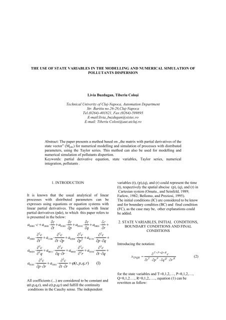
4. EXAMPLE FOR A DISPERSION OFINDUSTRIAL POLLUTANTSTo check the above mentioned modelling andnumerical simulation method the following cases areused.c(t,p)10.80.64.1 The Analytical Solution.0.40.2The analytical solution necessary for the start of theanalytical calculations and for the cumulativerelative error in percent (crep) is the following:02p[km]1.510.5000.20.40.60.81t[h]cAN= A⋅εt−tg 2−()σt⋅εp−pg2−()σp⋅εq−qg 2−()σq⋅εr−rg 2−()σr⋅k⋅u4.2 The Coefficients of the Analytical Solutionu(10)They are:A=1;σ t =0.5; σ p =0.5; σ q =0.5; σ r =0.8a 0000 =1; a 1000 =T1+T2; a 0100 =P1+P2; a 0010 =Q1+Q2;a 0001 =R1+R2;a 2000 =T1*T2;a 1100 =(T1+T2)*(P1+P2);a 1010 =(T1+T2)*(Q1+Q2);a 1001 =(T1+T2)*(R1+R2);a 0200 =P1*P2;a 0110 =(P1+P2)*(Q1+Q2);a 0101 =(P1+P2)*(R1+R2);a 0020 =Q1*Q2; (11)a 0011 =(Q1+Q2)*(R1+R2); a 0002 =R1*R2;andT1=0.1; T2=0.2; P1=0.15; P2=0.25; Q1=0.15;Q2=0.25; R1=0.04; R2=0.06;4.3 Cases Considered.We consider three usual cases described by thefollowing values.First case:t 0 = 0; t f = 1; t=0:0.05…1; r g =0; r 0 =0; r f =0.5 ;r=0:0.05…0.5; q 0 =0;q f = 0 ; q=q f ; p 0 =0; p f = 0; p = p f(the results are represented in figure 1.)10.80.60.40.200.8c(t,r)r[km]0.60.40.200Fig. 1. The variation of c[μg/m 3 ] forp=0[km],q=0[km], r=0-0.5[km] and t=0-1[h].Second case:t 0 = 0; t f = 1; t=0:0.05…1; q 0 =0; q f =0; q= q f ;p 0 = 0 ; p f =2; p=0:0.1…2; p g = 0; r 0 =0; r f = 0;r = r f(the results are represented in figure 2.)0.20.40.60.8t[h]1Fig. 2. The variation of c[μg/m 3 ] forq=0[km],r=0[km], p=0-2[km] and t=0-1[h].Third case:t 0 = 0; t f = 1; t=0:0.05…1; p 0 =0; p f =0 ;p=p f ; q g = 0;q 0 = 0 ; q f =2; q=0:0.1…2; r 0 =0; r f = 0.1; r = r f ;(theresults are represented in figure 3.)The time and space’s constants are: T 1 =0.1; T 2 =0.2;P 1 =0.15; P 2 =0.25; Q 1 =0.15;Q 2 =0.25; R 1 =0.04;R 2 =0.06 ; k u =1; u=1 for all the cases studied.c(t,q)10.80.60.40.202q[km]1.510.500Fig. 3. The variation of c[μg/m 3 ] forp=0[km],r=0[km], q=0-2[km] and t=0-1[h].4.4 Value of n,N,M.Values for the n, N and M are: n=2; N=3 ; M=6.4.5 The Cumulative Relative Error Percents.The accuracy of the numerical integration wasapproximated through the cumulative relative errorpercents defined by:tf∑t 00.2f∑ Δxt 0crepc = 100 ⋅tx0..0AN 0..00.40.60.81t[h](12)where:Δ x0 ..0= cAN − x0..0(difference betweennumerical and analytical solution in absolutevalues);

x =AN ..0c AN0corresponds to the analytical valueadding that (t∑ ft 0)is the iterative sum up of calculussequences from t0 to t f . The integration step is 0.001and the cumulative relative error percents is lessthen 0.02 percents . The following tabel showssome values of crepc.Table 2t 0.2 0.4 0.6 0.8 1c(t,p) 0.046 0.142 0.317 0.512 0.600crepc 5*10 -5 5*10 -5 5*10 - 5 1*10 -4 1*10 -4c(t,q) 0.049 0.152 0.339 0.547 0.641crepc 5*10 -5 5*10 -5 5*10 - 5 1*10 -4 1*10 -4c(t,r) 0.052 0.161 0.357 0.577 0.676crepc 5*10 -5 5*10 -5 5*10 - 5 1*10 -4 1*10 -45. CONCLUSIONSThis paper presents a possible numerical modellingand simulation variant with second order partialderivative equations, which depend on fourindependent variable . One of them (t), representstime and the other (p), (q), and (r), are usuallyconsidered spatial Cartesian coordinates.The paper defines and uses the „ matrix with partialderivatives of state vector” (M pdx ), associated to theTaylor series, dedicated to modelling and numericalsimulation of a large category of partial differentialequations.For the proposed variant we operate with timeconstants T 1 and T 2 and length constants P 1 , P 2 ,Q 1,Q 2 , R 1 , and R 2 . These constants are usually used inthermo-energetical and chemical engineering.Choosing those constants conveniently we canobtain a lot of geometry for dispersion pollutants.In this paper three examples which can approximatethe following situations are considered:- the source of the pollutants is a power plant stack;- the origin of the Cartesian system is on the top ofstack, which is the source of pollutants;-the pollutants dispersion is considered during 1hour and:- on 0.1 km upper stack (p=0; q=0; r=0-0.5) ( Fig. 1).-on 2km horizontal (p=0-2km, q=0km and r=0)(Fig. 2);- on 2km horizontal (q=0-2km, p=0km and r=0km)( Fig. 3);For the validation of the method and to determinethe performance of numerical integration theconstants in (11) have been used .Table 2 shows a cumulative relative error of c (crepc) equal with 5*10 -5 -10 -4 percents, whichdemonstrates the numerical integration performanceand validity.The commonly used method of modelling airpollutant dispersion is represented by a differentialequation, which expresses the rate of change ofpollutant concentration in terms of average windspeed and turbulent diffusion. Mathematically, thisprocess is derived from the mass conservationprinciple, (Mastoraks, 2004). The basic diffusionequation used in air quality modelling is given by:∂C∂C= −u⋅ + D∂t∂x222∂ C ∂ C ∂ Cx + D D2 y +2 z +2∂x∂y∂zw;(13)where:- C represents the concentration in atmosphericpollution (μg /m 3 );- D x ,D y , and D z represent the diffusion coefficients(m 2 /s);- u represents the wind speed (m/s);-w represents the mass of species due to chemicalreactions(kg/m 3 s);Equation (13) can be obtained from (1) by setting thecoefficients to particular values.This preliminary approximated work for pollutantsdispersion can be completed with details regardingmeteorological and terrain factors.Also, the work will be used for numerical modellingand simulation control system in reduced pollutantsindustrial processes.The accuracy of the numerical integration that wasapproximated through the (crepc), can be controlledand improved if N and M are chosen accordingly.REFERENCESBellomo, N., and L. Preziosi (1995). ModellingMathematical Methods and ScientificComputation , CRC Press Inc.Buzdugan, L., T. Coloşi, (2006). TheoreticalPreparatories Regarding Modelling andNumerical Simulation of Some DistributedParameters Processes, IEEE InternationalConferene AQTR Cluj-Napoca.Buzdugan, L., T. Coloşi, (2007). NumericalModelling and Simulation Variant forPollutants Spatial Dispersion, Proceeding ofInternational Conference CSCS-16 Bucharest.Coloşi, T., M. Abrudean, E.Dulf and M. Ungureşan(2006) . Numerical Modelling and SimulationMethod with Taylor Series, MediamiraScience Publisher, Cluj-Napoca .Farlow, S.J.(1982). Partial Differential Equations forScientists and Engineers, John Wiley and SonsInc.Henrici P. (1964). Discrete Variable Methods inOrdinary Differential Equations, John Wileyand Sons, New York.Mastoraks E., (2004) Dispersion of Pollution in theAtmospheric Environment, CambridgeUniversity Course.Omatu, S., and J. H. Seinfeld (1989). DistributedParameter Systems OHMSHA, ClaredonPress, Oxford.