Advance Modeling of a Skid-Steering Mobile Robot for Remote ...

More documents

Recommendations

Info

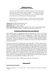
6.1 Simulink Model 84(a)(b)Figure 6.4: (a) Block scheme for the longitudinal reaction force; (b) Block scheme for the contact point dynamics.
6.1 Simulink Model 85as explained in Section 4.1. Such a dynamics of the contact point when the tire is releasingis so complex that it would require an ¨ad hoc¨ study, which is not provided in this thesis.In order to overcome this issue, we consider N ic = m t g and we assume that the conditionson F icx given in (4.13) still hold. However, when the value of F icx switches from F icx 0 toF icx = 0, the value for v icx could not be zero as it should be. In such a case, as the contactpoint dynamics switches from m t˙v icx 0 to m t˙v icx = 0, the velocity v icx will stay stable tothe value it had before switching, so that also the tire reaction force will keep its stable valueinstead of performing the expected stretching/releasing behavior. The solution to this issuecan be found by simply rewriting (4.13) as follows:f ix = −D x (∆v ix − v icx ) − K x∫(∆v ix − v icx )dtm t˙v icx + D x v icx + µ kx N ci sign(v icx ) = F icx′⎧⎪⎨ 0, for |FF icx ′ ix ′=| < µ sxN i ∧ f i (t − ∆t) = 0⎪⎩ Fix ′ , for |F′ ix | > µ kxN i ∧ f i (t − ∆t) 0∫F ix ′ = m t˙v ix + D x v ix + K x (v ix − v icx )dt(6.4)where f i = 1, 0 is a flag indicating whether the contact point is moving or not.We notice that, in this case, when the value of F icx switches from F ′ icx 0 to F′ icx= 0, thesecond equation in (6.4) represents an asymptotically stable system instead of a simply stablesystem, therefore v icx will tend to zero independently from the value it had before switching.Briefly, as we do not know the dynamics of N ci allowing the contact point to stop, we areimposing v icx = 0 when F ′ icx= 0. However, it must be noticed that the overall dynamicsdoes not change from the theoretical one, except for the fact that the contact point does notstop when Ficx ′ = 0 as for the theoretical case, but it stops some time later. Moreover, as weit will be shown in the next Section, the system represented by the second equation in (6.4)is over-damped, i.e. D x > 2 √ m t K x , and the corresponding time constant is relatively small,i.e.√mtK x≪ 0.1. As a consequence, the contact point stops immediately after F ′ icx= 0. Itis worth noticing also that such approximation of the contact point dynamics does not takeinto account the case in which v ix is relatively high, or N ci relatively low, so that v icx couldnever reach zero, as explained in Section 4.1. However, we are considering only the caseω z < 64 degs≈ 1 rad,that is v s ix < 0.15 m , and the acquired data from the force sensor alwaysspresents the saw-tooth shape when pulling the robot up to 0.1 m , therefore we can assumes
Page 1 and 2:
Università degli Studi di GenovaRo
Page 3 and 4:
IINothing great in the World has be
Page 5:
CONTENTSIV6 Simulation 786.1 Simuli
Page 8 and 9:
LIST OF FIGURESVII6.4 (a) Block sch
Page 10 and 11:
List of Tables5.1 Table of the geom
Page 12 and 13:
Introduction 2boDynamics, VGo Commu
Page 14 and 15:
Introduction 4The robot employed, i
Page 16 and 17:
Chapter 1Hardware and SoftwareIn th
Page 18 and 19:
1.1 The Pioneer 3-AT Robot 8four ho
Page 20 and 21:
1.2 The sensors 10control resolutio
Page 22 and 23:
2.1 State of the Art 12not negligib
Page 24 and 25:
2.1 State of the Art 14velocity vec
Page 26 and 27:
2.1 State of the Art 16Figure 2.3:
Page 28 and 29:
2.1 State of the Art 18Finally, by
Page 30 and 31:
2.1 State of the Art 20constraint (
Page 32 and 33:
2.1 State of the Art 22approximates
Page 34 and 35:
2.2 Generalized Modeling 24⎡1 0¯
Page 36 and 37:
2.2 Generalized Modeling 26V = [v T
Page 38 and 39:
2.2 Generalized Modeling 28where T(
Page 40 and 41:
2.2 Generalized Modeling 30⎡g R(J
Page 42 and 43:
2.2 Generalized Modeling 32where we
Page 44 and 45: Chapter 3Experimental DataIn this c
Page 46 and 47: 3.1 The accelerometer 36(a)(b)Figur
Page 48 and 49: 3.2 Characterization of the Vibrati
Page 54 and 55: 3.3 Characterization of the Tire Fo
Page 66 and 67: 4.1 Tire Lateral Force 56Figure 4.1
Page 68 and 69: 4.1 Tire Lateral Force 58velocity b
Page 70 and 71: 4.1 Tire Lateral Force 600 ≤ µ i
Page 72 and 73: 4.3 Tire Vertical Force 62f ix (t)
Page 74 and 75: Chapter 5Identification of the Robo
Page 76 and 77: 5.1 Identification of the Geometric
Page 78 and 79: 5.2 Identification of the Tire Dyna
Page 88 and 89: Chapter 6SimulationIn this chapter,
Page 90 and 91: 6.1 Simulink Model 80On the right h
Page 92 and 93: 6.1 Simulink Model 82Figure 6.3: Bl
Page 96 and 97: 6.1 Simulink Model 86that v icx can
Page 98 and 99: 6.2 Simulation Results 88(a)(b)Figu
Page 100 and 101: 6.2 Simulation Results 90enough to
Page 102 and 103: 6.2 Simulation Results 92hand side
Page 104 and 105: 6.2 Simulation Results 94(a)(b)Figu
Page 106 and 107: 6.2 Simulation Results 96• For λ
Page 108 and 109: AppendixesAppendix A1 %% Main progr
Page 110 and 111: Appendixes 10080 title([conf,’; A
Page 112 and 113: Appendixes 10224 Hd = design(h,filt
Page 114 and 115: Appendixes 1043031 % Filter the dat
Page 116 and 117: Appendixes 106(a)(b)(c)Figure 6.10:
Page 130 and 131: Appendixes 120(a)(b)Figure 6.24: Pe
Page 144 and 145:
Bibliography[1] G. Oriolo, A. De Lu
show all

Advance Modeling of a Skid-Steering Mobile Robot for Remote ...

You also want an ePaper? Increase the reach of your titles

Delete template?

Save as template?