Potential Vorticity Inversion - F9

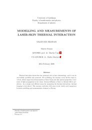
Potential Vorticity InversionLina BoljkaMentor: prof. dr. Nedjeljka ŽagarFaculty of Mathematics and PhysicsUniversity of LjubljanaMay 29, 2012AbstractIn this seminar are presented some typical meteorological terms, that have significant impact on derivingthe flow structure. Firstly, there is included the potential vorticity conservation law, which holds onlyin the adiabatic and frictionless atmosphere, because advective processes exceed diabatic and frictionalones. Secondly, there is introduced the invertibility prinicple of isentropic potential vorticity distribution,which states, that if the total mass under each isentropic surface is specified, then the global distributionof potential vorticity and of potential temperature at the lower boundary is enough to derive wind,temperature, pressure and vertical velocity fields. There are also included some examples, such as thestructure and persistence of cutoff cyclones and blocking anticyclones, which are described with isentropicpotential vorticity maps.1 IntroductionIt has been proven in the last few decades, thatisentropic potential vorticity (IPV) is very importantfor understanding mid-latitude weathersystems.Potential vorticity (PV), in general, is importantas an air-mass tracer for adiabatic, frictionlessflow and is therefore important to define an airparcel.More significant value of PV we get, when wedraw the isentropic potential vorticity maps fromwhich we can see, that the PV could also be usedto determine upper air winds, since the transportof PV affects the wind-field. In order to deducethe complete flow structure (temperature, windand pressure field) from the spatial distributionof PV, we shall use the invertibility principle.Normally we would take the 300K-350K potentialtemperature surfaces, which are on theboundary of troposphere and stratosphere, to determinewhich air was of stratospheric origin, tofind upper tropospheric front. When the stratosphericair enters troposphere, it could be advecteddown causing isentropic surface to slopeto altitudes that are usually considered to betropospheric, which can be shown with verticalcross-sections.Furthermore, PV anomalies in upper tropospherecould also be used to explain the observedcyclogenesis events, which are caused by injectionof high PV polar air from polar front.In the early 1980s the IPV maps have also beenincluded into the atmospheric model simulations,studies of oceanic circulations and in diagnosis ofobserved atmospheric behaviour.In this seminar, which is primarily based on articleby Hoskins et al. (1985), I will thus representpotential temperature, isentropic potential vorticity,its invertibility principle and present itssruface maps on examples, such as developmentof a North Atlantic cutoff cyclone, a minor block-1

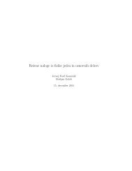
Potential Vorticity Inversion May 29, 2012ing episode and heavy-rains in Alpine south-side. 2.2 Isentropic coordinate system2 Potential temperature2.1 DefinitionAccording to Holton (2001), potential temperature,θ, is a temperature that a parcel of dry airwould have if it were expanded or compressedadiabatically to a standard surface pressure p s =1000hPa. We derive θ from thermodynamic energyequation per unit massdTc pdt − αdp = J, (2.1)dtwhere c p = 1004 JkgKis specific heat of dry airat constant pressure, T temperature, p pressure,α = 1 ρ= RTpspecific volume, R = 287.04 JkgKspecific gas constant for dry air, ρ density, J =dQdtheating rate and Q heat. We get this formof thermodynamic equation if we take a totalderivative of equation of state 1 ,using the relationpα = RT, (2.2)c v + R = c p (2.3)and apply it to the first law of thermodynamics2 . Dividing (2.1) by T , and assuming thatlarge scale (synoptic) motions are approximatelyadiabatic, we may take J T = dSdt= 0, where S isenthropy, and integrate (2.1)∫ Tθd ln T = R c p∫ pwe get the equation for θθ = Tp sd ln p, (2.4)( ) (R/cp) ps, (2.5)pthat is quasi-conserved for synoptic-scale motions.1 α dp+ p dα = R dT2 dt dt dtdTc v + p dα = J, where cv is specific heat of dry airdt dtat constant volumeFor adiabatic motions it is useful to take θ asvertical coordinate, since it is conserved folowingthe motion. We call the (x, y, θ) system isentropiccoordinate system. Thus the isentropesare lines of constant θ and isentropic surfacesare the surfaces of contant θ.For further derivations we will need the pressuregradient force per unit mass in cartesian coordinatesystem− 1 ρ ∇ hp (2.6)( )expressed in terms of θ, where ∇ h = ∂∂x , ∂∂y.Therefore we take transformation from z to θcoordinate system:∇ h p| z = ∇ h p| θ − ∂p∂z ∇ hz| θ , (2.7)where we use hydrostatic equation∂p∂z= −ρg, (2.8)the equation for geopotential φ = gz and we derivep from (2.5) and apply these terms in theequation (2.7). We get the pressure gradientforce in isentropic coordinate system−∇ h MM = c p T + φ,(2.9a)(2.9b)where M is Montgomery streamfunction.We will also need the equation for gradient windin natural θ coordinate system. Gradient windis approximation of the wind flow on curvedstreamline around the trough (cyclone) or ridge(anticyclone) in the upper troposphere. We cancompute gradient wind using pressure gradientforce, F p , in θ coordinate system, centrifugalforce F φ = v2rand Coriolis force F c = fv, wheref = 2Ω earth sin φ Coriolis parameter and φ latitude.The balance of these forces in cyclone isshown in Fig. (1), from which we can derive:2v 2r+ fv =∂M∂r . (2.10)

Potential Vorticity Inversion May 29, 20123.2 Barotropic systemBarotropic system is the system in which thereis no vertical motion, since the density dependsonly on the pressure ρ = ρ(p), so that isobaricsurfaces are also surfaces of constant ρ. Inisentropic coordinates we derive from equations(2.2), (2.3) and (2.5) the equation for ρ:p cv/cpρ = pR/cp s, (3.3)θRwhere one can see, that ρ is dependent only onp.3.3 Bjerknes’ circulation theoremFigure 1: Figure shows balance of pressure gradientforce, Coriolis force and centrifugal force per unitmass. Source: [5]3 Ertel’s potential vorticity3.1 VorticityAccording to Holton (2001), vorticity is the microscopicmeasure of rotation in a fluid and isdescribed as a vector field defined as the curl ofvelocity. The absolute vorticity η is the curl ofthe absolute velocity, whereas the relative voriticityζ is the curl of the relative velocity, in whichwe are concerned only with the vertical componentsof the vorticity. Therefore we getη = k·(∇ × U a ),ζ = k·(∇ × U),(3.1a)(3.1b)where U a is absolute velocity and U relative velocity.The difference between η and ζ is planetaryvorticity f (η = ζ + f), which is the localvertical component of the vorticity of the earthdue to its rotationf = k·(∇ × U e ) = 2Ω sin φ, (3.2)where U e is the velocity of Earth at certain radius.According to Holton (2001), the circulation, C,about a closed contour Γ in a fluid is definedas the line integral evaluated along the contourof the component of the velocity vector that islocally tangent to the contour:∮C = U·dl. (3.4)ΓThe circulation in relative system is expressed asC relative = C absolute − C earth ,dCdt = dC a− dC edt dt ,∮dC dpdt = − ρ − 2ΩdA edt , (3.5)where the later is called Bjerknes’ circulationtheorem. To derive the later we used equationsof motiondU a= − 1 ∇p + g,dt ρdU e= 2Ω sin φ dAdtdt , (3.6)where A is the area of vortex on Earth’s surfaceand A e = A sin φ is projected area. For abarotropic fluid one may see, that − ∮ dpρ = 0,since we have the integral about closed loop, forexample, if we apply the equation (3.3) to thisintegral we get −const. ∮ dpthe equation (3.3) becomesdCdt + 2ΩdA edtcv1− cp= 0. Therefore= 0. (3.7)3

Potential Vorticity Inversion May 29, 20123.4 Stokes’s theoremdefined with minus so that it is normally positivein the Northern Hemisphere. Potential vorticityis thus conserved following the motion inStokes’ theorem may be written as∮ adiabatic frictionless flow. However, normallyU·dl = (∇ × U) ·n dA, (3.8) we use the term potential vorticity, when referringto the ratio between the absolute vorticityΓAand effective depth of the vortex, for example in(3.12) the effective depth is correlated with staticstability parameterwhere we can find the relation between relativecirculation and relative vorticity. Thus, accordingto Holton (2001), the circulation about anyclosed loop is equal to the integral of normalcomponent of vorticity over the area enclosed bythe contour C = ζdA. (3.9)AHence, for finite area, circulation divided by areagives average normal component of vorticity inthe region¯ζ = δC (∮δA = limA→0)U·dl A −1 . (3.10)σ = − 1 g∂p∂θ> 0. (3.13)From these assumptions we may derive PV conservationequation for homogenuous incompressiblefluid, where ρ is constant, M = ρhδA isconserved, A = const./h, where h is the depthof the parcel, therefore we getP V = ζ + fh= Const. (3.14)3.5 Potential vorticity (PV)Using equation (3.7) for barotropic isentropicsystem and inserting relations (3.10) and theCoriolis parameter f, we getddt ((ζ θ + f)δA) , (3.11)where ζ θ is vertical component of relative vorticityon isentropic surface. Supposing that theparcel of air is confined between potential temperaturesurfaces θ 0 and θ 0 + δθ, seperated bypressure interval −δp, the mass of this parcel,δM = ρδzδA, must be conserved following themotion. From hydrostatic equation (2.8) we getδA = −g δM δθδp δθ , since δM δθis constant, the equation(3.11) becomes, when δθδp → 0,(P = (ζ θ + f) −g ∂θ )= const., (3.12)∂pwhich we call Ertel’s or isentropic potential vorticityand we measure it with PVU (potentialvorticity unit), where 1PVU is 10−6 Km2kgs . P is4 Invertibility principleIsentropic potential vorticity maps are a diagnostictool, that makes dynamical processes visibleto human eye and therefore allows us to makecomparissons between real state and model calculations.They improve our understanding ofdynamical processes. To support these statementswe use Lagrangian conservation propertiesand the invertibility principle. In the barotropicmodel one can deduce the streamfunction byinverting a Laplacian operator, which gives uswind field. Thus we may think only in terms ofthe PV field, like they used to do it in aerodynamics.The invertibility principle requests determiningthe 2 factors of IPV seperately - absolutevorticity and static stability - for whichwe need some more information, as described inHoskins et al. (1985):(i) specify some kind of balance condition,for which the simplest, but least accurateoption, is ordinary geostrophic balance(fU g = 1 ρ k × ∇p),4

Potential Vorticity Inversion May 29, 2012(ii) specify some kind of reference state, expressingthe mass distribution of θ, whichwe could take from climatological data,(iii) solve the inversion globally, with properboundary conditions.5The first 2 points imply, that we have to speak ofinversion under specified balance condition andrelative to specified reference state, while thethird point states, that we can only find a pairof absolute vorticity and static stability whentaking global distribution, since we cannot determinethem seperately by local distribution ofIPV, since we would have to take into accountalso the side conditions. We must assume, thatinstabilities, such as static or inertial instability,are absent, which is compatible with large(synoptic) scales and motions moving upwards.Those models tend to be insensitive to the detailsof fine structure - we make ’coarse-grain’approxiamtions to IPV.To derive the IPV inversion we will assume, thatwe have horizontally uniform reference state,constant Coriolis parameter f and that hydrostaticpressure field p is a function of θ, p =p ref (θ), which is monotonically decreasing withheight so that reference state is statically stable.These assumptions lead to constant PV for referencestate on each isentropic surface P ref (θ). Werequire that the actual state has the same massdistribution as reference state (mass lies betweenθ and θ+dθ) expressed in isentropic coordinates:∫ ∫ ∂p(x, y, θ)dxdy = dp ∫ ∫ref (θ)dxdy,∂θdθ(4.1)which is taken over a horizontal domain, muchlarger than the size of the IPV anomaly. Thissatisfies the condition (ii).If we assume further on that PV anomaly iscircularly symmetric on some of the isentropicsurfaces, wind, pressure and temperature fieldsbecome circularly symmetric, and if we neglectfriction and diabatic heating, the flow becomessteady, nondivergent and purely azimuthal. Weget horizontal wind speed, v = v(r, θ), dependentonly on θ and r (horizontal distance fromthe centre of anomaly). The balance conditions(i) therefore become the gradient wind equationand hydrostatic relations. If we write these conditionsin terms of θ and Montgomery streamfunction M(r, θ) from equation (2.9b), we mayrewrite gradient wind equation from (2.10) as∂M(r, θ)∂r≡(f + v )v (4.2)rand the hydrostatic equation (2.8) as∂M(r, θ)∂θ≡ c p( pp 0) r/cp≡ Π(p), (4.3)where Π(p) is called Exner function, p 0 =1000mbar. Now we eliminate M by makingcross-differentiation on equations (4.2) and (4.3)to derive:where R(p) represents(f + 2 v ) ∂vr ∂θ = R(p)∂p ∂r , (4.4)dΠ(p)dp . (4.5)Taking equations (3.12) and (3.13), whereη θ = f + ζ θ (4.6)and the relative isentropic vorticity, given by(3.1b), can be rewritten in terms of circular symmetryand constant θWe get the potential vorticity−1 ∂(rv)ζ θ = r∂r . (4.7)P (r, θ) = σ −1 η θ . (4.8)Taking these assumpition into account, we areable to express invertibility principle the followingway. If we differentiate equation (4.8) withrespect to r and put it in the equations (4.6),

Using equations (4.10), (4.8), we can rewriteequation (4.9) as[ ][ ]∂ 1 ∂(rv)+ g −1 P ∂ f +2vr ∂v= σ ∂P∂r r ∂r ∂θ R ∂θ ∂r ,(4.11)which is a non-linear equation that can be solvedby iteration for wind profile v(r, θ) with givenIPV distribution P (r, θ). Note that the isentropicgradient of P appears on the right-handside as a prescribed forcing function. Also for(f + 2vr)P > 0 we assume, that equation (4.11)is an elliptic equation so that the problem is welldefined. If we make further assumptionsf + 2vr ≈ η θ ≈ f,R ≈ R ref (θ),σ ≈ σ ref (θ) (4.12)everywhere except when calculating ∂P∂rfromequation (4.8), where σ ref and R ref are the referencestate profiles of R and σ, we may simplifyequation (4.11) to[∂ 1∂r r+]∂(rv) f 2∂r gσ ref[ ]∂ 1 ∂v ∂P= σ ref∂θ R ref ∂θ ∂r .(4.13)One may see, that the elliptic operator on theleft-hand side is now linear, and we may makefurther assumptions, to make calculations easier,like σ ref and R ref being constant, even thoughthe differences in these parameters are very importantnear fronts and shear lines. If we suitablyrescale the vertical coordinate we get an operatorthat has some resemblance with Laplace6Potential Vorticity Inversion May 29, 2012(4.7), assumimg that f is constant, and multiplyingthe result by σ, we getHaving made these assumption we may now startoperator ∇ 2 , which is elliptic.[ ]∂ 1 ∂(rv)− η θ ∂σ∂r r ∂r σ ∂r = σ ∂Pthe simplest, but not the most powerful method∂r . (4.9) with iteration described in Hoskins et al. (1985):we start with equation (4.13) as first guess, whichimproves the initial approximations (4.12) byIf we also differentiate (3.13) with respect to rstraightforward iteration. As soon as we com-and use equation (4.4), we get[ ]−g ∂σ∂r = ∂2 p∂r∂θ = ∂ f +2vr ∂v. (4.10)∂θ R ∂θpute a guess for v(r, θ) from (4.11), using theprevious guesses for R and σ, improved approximationsto them must be derived for use in thenext iteration. Integrating (4.2) with respect tor, and afterwards using (4.3), (3.13) and (4.5),we can derive p(r, θ), R and σ. When integrating(4.2) with respect to r, we get a function dependenton θ as a function of integration, thus weneed to use reference-state condition (4.1) andboundary conditions to determine this functionof integration.Figure 2: Figure shows circularly symmetric flows inducedby IPV anomalies (stippled regions). The thickline represents the tropopause and the two sets ofthin lines the isentropes every 5K and the transversevelocity every 3 m/s. In (a) the azimuthal wind is cyclonicand in (b) it is anticyclonic. Source: Hoskinset al. (1985), Fig. (15).

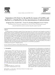
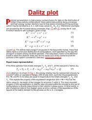
Potential Vorticity Inversion May 29, 2012The result of such invertibility principle is shown the anomaly (statements (i) and (ii)), thereforein Fig. (2), which uses boundary conditionsthe static stability must deviate in thev → 0 if r → ∞ and θ = const. at 60 and1000mbar, showing the flow structures caused byisolated, upper-air PV anomalies, where the example(a) in the Fig. shows the flow, caused bypositive (cyclonic) anomaly, while (b) is causedoposite sense in order to compensate. Sincethe P appears partly as η θ and partly as σ,broad, shallow anomaly thus tends to realizeP more as static stability and a tall onemore as absolute vorticity.by negative (anticyclonic) anomaly, which hasa larger radial extent. The reference state p =There is also seen a similar anomaly in thep ref (θ) consists of two layers with differing staticboundary, that causes cyclonic or anticyclonicstabilities representing troposphere and strato-vortex in the boundary.sphere. In the model, there was also used thepotential temperature } anomaly in tropopause asθ ′ = 1 2{cos A π˜rr 0+ 1 for ˜r < r 0 , where A is−24K in (a) and +24K in (b), ˜r = r√f+(2v)/rf.One may also see, that the values of f + 2vrandη θ greatly exceed f near the centre of the cyclonicvortex. For this reason some other theoriesare poor approximations, e.g. so-called semigeostrophicand quasi-geostrophic theory. As describedin Hoskins et al. (1985), what one mustnote about Fig. (2) are the following points:(i) the circulation (the same as azimuthal wind,therefore also relative vorticity) in the balancedvortex has the same sense, relative tothe earth, as the IPV anomaly which causedit;5 Isentropic potential vorticitymapsThere are given several isentropic potential vorticitymaps for different isentropic, pressure andgeopotential height surfaces from 20 th of Septemberto 31 st of October 1982. The data sourcewere daily products of ECMWF (European Centrefor Medium Range Weather Forecasts). To(ii) the induced fields penetrate vertically aboveand below the IPV anomaly, since the effectof IPV anomaly cannot be limited only tosuch a small area;(iii) the static stability, as well as absolute vorticity,is anomalously high within a high PVanomaly and vice versa in low PV anomaly,relative to the static stability of the refernecestate, which can be seen from θ contoursin Fig. (2) being closer together instratosphere than in troposphere;(iv) the static stability anomalies have the oppositesense to the IPV anomaly in the regionsabove and below that anomaly, because η θstill has the same sense above and bellowFigure 3: Figure shows the potential vorticity distributionwith height and latitude. Isentropic surfacesare shown as: × (350K), • (330K), + (315K) and ◦(300K). Source: Hoskins et al. (1985), Fig. (1).cunstruct IPV objectively on isobaric surfacesthere were used centred finite differences and linearinterpolation to derive velocity, IPV and potentialtemperature surfaces. Note that thesecan only make a coarse-grain approximation,since the data was analysed isobarically ratherthan isentropically. The values of IPV are givenin PVU, which corresponds to changes in θ for7

Potential Vorticity Inversion May 29, 201210K/100mbar.for days, or sometimes may move in the oppositeFrom Fig. (3) we can see that tropospheric direction.values are generally below 1.5PVU, while intropopause (narrow part of lines) they suddenlyrise for about 4PVU. One may also see that valuesof θ = 350K, marked with crosses, fall totroposphere when moving towards equator, andto stratosphere when moving towards the pole.This is how we differ stratospheric and troposphericair in our IPV maps.Investigating the given period, there were foundtwo specific developements, the formation of cutoffcyclone and blocking anticyclone in middleand high latitudes - in the North Atlantic. Theseoccurances are investigated for they may causeplenty of precipitation (cyclone) or sunny days(anticyclone).Figure 5: Figure shows the 500mbar geopotentialheight maps for the period 20-25 September 1982.The contour intervals are 100m. Source: Hoskins etal. (1985), Fig. (6).Figure 4: Figure shows the 300K IPV maps for theperiod 20-25 September 1982. The contour intervalsare 0.5 PVU. Source: Hoskins et al. (1985), Fig. (5).5.1 Development of a North Atlanticcutoff cycloneCutoff cyclone is a closed low which has becomecompletely cut off from the basic westerly current(mid-latitudes) and moves independently ofthat current. They may remain nearly stationaryIt is often accompanied by a blocking high.Note that the use of ”cut-off low” is reservedfor those closed lows which are clearly detachedcompletely from the westerlies.From Fig. (4), which represents IPV anomalieson 300K surface for 20 th to 25 th of September1982 between 120 o W and 0 o W longitude,and region north of 40 o N latitude, one maysee that a 300K surface intersects with stratosphereon 20 th of September on the left of themap, which corresponds to large PV gradients,shown as a thick line of 1.5-2PVU. In the periodof 21-23 September a large piece of highPV moves rapidly eastwards, what seems to havebeen caused by advection of strong upper-airwinds. On 24 th of September it has cut off andbecame its own cyclonic circulation. On 25 thof September the feature has already weakened.There are also included corresponding 500mbargeopotential height fields, Fig. (5), that show asmoothed view of the same process, where there8

Potential Vorticity Inversion May 29, 2012Figure 6: Figure shows the 1000mbar geopotentialheight (a) and 700mbar (b) temperature maps for theperiod 22-24 September 1982. The contour intervalsare 60m and 5K, respectively. Source: Hoskins et al.(1985), Fig. (7).Figure 7: Figure shows a vertical section through acutoff cyclone on November 16, 1959. The thick linerepresents tropopause, dashed lines are isotherms andsolid lines isentropes. Contour intervals are 5 o and5K, respectively. Source: Hoskins et al. (1985), Fig.(8).is also a form of cutoff cyclone on 24 th of September.The 1000mbar height maps, Fig. (6), showa rapid developement of low-level cyclonic circulationbetween 22-24 September without lowleveltemperature field changes until late in period,when cold air sits over the low pressure.The vertical structure of such cutoff cyclone isshown in Fig. (7), which was represented in 1963by Peltonen, and shows significant resemblancewith Fig. (2), which was computed using invertibilityprinciple.The idea of cutoff cyclones is also related to phenomenonof Alpine lee cyclogenesis.5.2 A minor blocking episodeA blocking anticyclone is a similar phenomenonas cutoff cyclone, only that it stands for highpressure vortices, that can also remain stationaryfor days and get cut off.A blocking episode occured in the period 30September - 7 October 1982. In Fig. (8) thereare shown 330K IPV maps with longitudes between60 o W and 60 o E and latitudes from 30 o Nto 80 o N. One may see a strong cyclonic vortexon the left of the map for 30 th of September,which causes strong south-westerly winds aheadof this system, which are very effective in advectinglow-PV air polewards, even more whenthey get additional force from the anticycloniccirculation that develops around this movinglow-PV air. By the 2 nd of October it has reached70 o N and has started to cut off. On the 3 rdof October it has already cut off with its ownstrong anticyclonic circulation, leaving a largepool of low PV inside its vortex. Afterwards itmoves a bit southwards, eastwards until, on 7 thof October, it finally links back to subtropicalair. On the 4 th and 5 th of October there comesanother blocking episode on the west fromprevious one, which would become cut off onthe 8 th of October. The same patterns are seen9

Potential Vorticity Inversion May 29, 2012Figure 8: Figure shows the 300K IPV maps for theperiod 30 September to 7 October 1982. The contourintervals are 1 PVU and the regions of 1-2PVU areblacked in. Source: Hoskins et al. (1985), Fig. (11).Figure 9: Figure shows the 250mbar geopotentialheight maps for the period 30 September to 7 October1982. The contour intervals are 100m. Source:Hoskins et al. (1985), Fig. (12).on the 250mbar geopotential height maps, Fig.(9), with somewhat smoothed version of IPVmaps represented before. The Fig. (10) showsthe 1000mbar height and 700mbar temperaturefor 2 nd of October, where one may see the deepvertical scale of the poleward flow of subtropicalair. The low-level temperature proves themovements of subtropical air mass seen in Fig.(8).There were 3 repeated incursions seen from 25 thof September to 8 th of October 1982, whichseem to be typical.Similar phenomena are observed in oceancurrents, e.g. ’Gulf Stream rings’, which alsoaffects the climate, especially in Europe andNorth America.also great resemblance with Fig. (2b), whichwas derived from PV anomaly of the oppositesign. Since we have neglected all frictional anddiabatic processes, these statements were true,but taking into acount also these processes thesimilarity ends. Diabatic heating dissipatesmore efficiently the positive IPV anomalies dueto bigger gradients in cyclones due to moisture,while radiative cooling dissipates negative IPVanomalies much more slowly, what gives theseanticyclones a blocking character. Friction canonly have some influence in the boundary andcannot cancel the whole vortex.One could also see their expansion to thesurface, causing cold or warm air penetratingtowards surface.Having presented cutoff high and low, I believewe could see the similarity in their occurance.This can also be proven by Fig. (11), whichseems to be right the opposite of Fig. (7). It has10

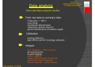
Potential Vorticity Inversion May 29, 2012form of an elongated filament of intruded stratosphericair that lies behind and parallel to thesurface front and extends south to the Mediterraneansea. The assumption was that the advectionof an upper-level PV anomaly toward theAlps is the main cause to the onset of severerainstorms on the southern slopes of mountainrange, which is connected to the the flow andthermal structure, which induce the heavy precipitation,by the invertibility principle of PV.Figure 10: Figure shows the 1000mbar geopotentialheight (a) and 700mbar (b) temperature maps for 2 The conditions that have to be met are there-October 1982. The contour intervals are 60m and5K, respectively. Source: Hoskins et al. (1985), Fig.(13).Figure 11: Figure shows a vertical section through acutoff anticyclone on 4 October 1982. The light continuousline represents isentropes every 10K, dashedline is PV of value 0.5PVU and heavy solid lines PVcontours every 1PVU. Source: Hoskins et al. (1985),Fig. (14).5.3 Alpine south-side precipitationNowadays, the researchers in Zürich are dealingwith heavy-rains in Alpine south-side, whichis described in article by Fehlmann and Quadri(2000).The research was ignited by bad forecasts forthe southern region of Alps, where there couldfall nearly 200mm in 24 hours, particularly duringfall, and would be very useful to know theamount of rain that is about to fall. Such stormsare caused by a moisture pre-frontal southerlyair-flow colliding with the main Alpine ridge andby a deep trough at a tropopause level in theFigure 12: Figure shows the upper-level PV structurefor 1800 UTC 4 November 1994 (upper panels) andpredicted 24 hour accumulated precipitation for theaccumulation period 0600 UTC 5 November to 0600UTC 6 November (lower panels) for two forecasts ofdifferent duration. Panel a) is a forecast initialized at0000 UTC 4 November, panel b) is the initial state.Source: Fehlmann and Quadri (2000), Fig. (1).fore:(i) strengthening of the southerly flow componenttoward the Alps;(ii) reduction of the static stability beneath theanomaly;(iii) upward movement on the forward flank ofstream to cause or strengthen and sustainconvection.11

Potential Vorticity Inversion May 29, 2012The analysis of these events is highly connectedto the PV distribution of the filament atthe initial time (the difference of the upper-levelPV as shown in Fig. (12)). To derive this initialfield we especially need to isolate the particularPV-element in the difference field, inverting thiselement to derive an estimate of flow field, whichwe use together with analysis of the flow to getfinal initial conditions.The paper further on shows, that the correlationof the forecast precipitation error and PVanomalies is high and thus the latter are cruicialin forecasting the precipitation in this region.subtropical and tropical latitudes. The inducedfield of any large-scale IPV anomaly, whatever itsorigin, may extend into middle latitudes causingthe tropics to appear as an absorber or reflectorof mid-latitude planetary-scale distrubances.Note that if the isolated vortex crosses the equatorinto the opposite hemisphere it would notchange its direction and would remain stable.The IPV maps looked very usefull in themid 1980s, their research reached the peak in1990s, while nowadays they are dealing withIPV anomalies especially in Zürich, in connectionwith heavy-rains in Alpine south-side, whichare believed to be caused by the advection of an6 Conclusionsupper-level PV anomaly from the north towardthe Alps.We have introduced the terms of potential temperatureθ, potential vorticity IPV, its variabilityand use. We have learnt that IPV inversionis a very quality approach for understanding ofdistribution of mass and wind fields. The IPVmaps help us to understand the general circulationof the atmosphere and give us the insight tothe general dynamics that occure in the atmosphere.With these maps we can analyse, for example,why are the maximum winds when frontoccurs, why is it when the θ contours have thestrongest tilt. We can also analyse the extremeevents with them to produce the scenario for theyears to come.The invertibility principle is very important inmeteorology, since it derives stability and wind,pressure and temperature fields from only onequantity, potential vorticity.Furthermore, the invertibility principle suggeststhat IPV concept remains useful even in the presenceof moist or dry diabatic heating or coolingand friction, because the basic balances still apply,though there could be argued whether or notwe got the correct diabatic and frictional rates ofchange of IPV distributions.One of the most useful describtions, that is givenby IPV maps, is therefore, that we may find reoccurancesof low-PV air being injected to middleand high latitudes and high-PV air moving toReferences[1] Falko J., Painemal D., Gramer L. andMantsis D.; Potential Vorticity in the Atmosphere,Class project[2] Fehlmann R., Quadri C.; Predictability Issuesof Heavy Alpine South-Side Precipitation,Meteorol. Atmos. Phys. 72 (2000), pp.223-231[3] Holton, J.R.; An Introduction to DynamicMeteorology, Academic Press, Inc., fourthedition, 2004, pp. 1-181[4] Hoskins, B.J., McIntyre, M.E., Robertson,A.W.; On the use and significance of isentropicpotential vorticity maps, Quart. J.R.Met. Soc. (1985), 111, pp. 877-946[5] http://www.aviamet.gr/cms.jsp?moduleId=009extLang=LG[6] http://www.weatherzone.com.au/help/ glossary.jsp?l=c[7] http://en.wikipedia.org/wiki/Cyclogenesis[8] http://en.wikipedia.org/wiki/Block %28meteorology%2912