2. STEADY FLOW, CONSTANT D, GIVEN n In this ... - ROOT of content
2. STEADY FLOW, CONSTANT D, GIVEN n In this ... - ROOT of content 2. STEADY FLOW, CONSTANT D, GIVEN n In this ... - ROOT of content
2. STEADY FLOW, CONSTANT D, GIVEN nIn this chapter three types of aquifers physically different, but mathematicallyidentical, will be examined.1. A phreatic aquifer with constant thickness D (as an approximation). - The laws oflinear resistance and continuity read respectively:Since for steady flow acp/at = O, the general formula N = n - p (acp/at) reduces toN=n.2. A partly confined aquifer. - The differential equations are the same. The expressionfor N reads for steady flow:The method of solution varies according to the way the problem is defined.- If n is given as a function of x and y, the first two members of the above expression,in combination with the differential equations, define the problem in exactly the sameway as in the case of a phreatic aquifer. The method of solution is identical, and givescp as a function of x and y. Once cp is known, cp’ can be determined;also as a function35
- Page 2 and 3: of x and y, from the last two membe
- Page 4 and 5: 1 As regards the quantitiesI'~Iir '
- Page 6 and 7: It follows that System 111 is defin
- Page 8 and 9: flow vector at any point of the bou
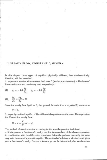
- Page 10 and 11: An0t t?Ep2PZnu 0OOp2I90p2Fig. 134Th
- Page 12 and 13: System 1:- Recharge n.- Potentials
- Page 14 and 15: Substituting successively1 forr=r,
- Page 16 and 17: Qo = nR2nSince Q, is given, this eq
- Page 18 and 19: Fig. 17.- Potential cpc at infinite
<strong>2.</strong> <strong>STEADY</strong> <strong>FLOW</strong>, <strong>CONSTANT</strong> D, <strong>GIVEN</strong> n<strong>In</strong> <strong>this</strong> chapter three types <strong>of</strong> aquifers physically different, but mathematicallyidentical, will be examined.1. A phreatic aquifer with constant thickness D (as an approximation). - The laws <strong>of</strong>linear resistance and continuity read respectively:Since for steady flow acp/at = O, the general formula N = n - p (acp/at) reduces toN=n.<strong>2.</strong> A partly confined aquifer. - The differential equations are the same. The expressionfor N reads for steady flow:The method <strong>of</strong> solution varies according to the way the problem is defined.- If n is given as a function <strong>of</strong> x and y, the first two members <strong>of</strong> the above expression,in combination with the differential equations, define the problem in exactly the sameway as in the case <strong>of</strong> a phreatic aquifer. The method <strong>of</strong> solution is identical, and givescp as a function <strong>of</strong> x and y. Once cp is known, cp’ can be determined;also as a function35
<strong>of</strong> x and y, from the last two members <strong>of</strong> the equation. If, for instance, the distribution<strong>of</strong> n over the aquifer is uniform, the value <strong>of</strong> cp' - cp is constant. <strong>In</strong> geometricalrepresentation: the cp' surface is at a constant height above the cp surface.- If cp' is given as a function <strong>of</strong> x and y, or as a constant, the problem assumes anothercharacter. The two differential equations are then to be combined withk'A; = -- (cp' - cp)D'and cp must be determined as a function <strong>of</strong> x and y by means <strong>of</strong> a different integration.Once cp is known, n can be found as a function <strong>of</strong> x and y fromProblems <strong>of</strong> <strong>this</strong> kind will be examined in Chapters 4 and 7.3. A confined aquifer. - The recharge n is zero because <strong>of</strong> the impermeable cover.The differential equations are the same as those <strong>of</strong> a phreatic aquifer, whileN=n=O<strong>2.</strong>1 SUPERPOSITION<strong>2.</strong>1.1 The principle<strong>In</strong> the following chapters the principle <strong>of</strong> superposition will be frequently used.Since its application varies according to the nature <strong>of</strong> the aquifer, its precise formulationwill be given in each chapter separately. <strong>In</strong> the present chapter the problem willbe limited to steady flow in aquifers with constant thickness D, where n is a givenfunction <strong>of</strong> x and y. The principle will be shown in an example.L Fig. 101Figure 10. - To give the example a general character, boundaries <strong>of</strong> different natureare assumed: an impermeable rock wall I, two rivers R and a lake L (a lake ratherthan :the sea, to avoid the complications <strong>of</strong> salt water intrusion). From <strong>this</strong> aquiferwater.is extracted by means <strong>of</strong> a number <strong>of</strong> wells.36
This description defines what will be called a model, <strong>this</strong> term taken in the sense<strong>of</strong> any material arrangement, either in nature or in the laboratory. On the givenmodel several flow systems can be imposed, defined by the following hydraulicdata :- The recharge n as a function <strong>of</strong> x and y.- The water levels in the rivers and the lake, determining cp along the borders.. t- A given supply <strong>of</strong> water along the :. rocky . . outcrop Z, as a function <strong>of</strong> the length coör->.. . , ...Idinate along <strong>this</strong> boundary. . .- The rates <strong>of</strong> extraction from the weilsl'"' .An arbitrarily chosen set <strong>of</strong> these values'defines a flow system, which means mathematicallythat at each point (x, y) the values <strong>of</strong> cp and q (qx and q,,) are determined.The principle <strong>of</strong> superposition can be formulated as follows: If in a certain model twodifferent flow systems, I and TT, can be realised, it is also possible to realise a thirdsystem, ITI, in which the values <strong>of</strong> cp, q and n at each point are the sum <strong>of</strong> the correspondingvalues in Systems I and 11. FOI cp and n <strong>this</strong> is the algebraic sum, for q thevectorial sum.This summation applies to all points <strong>of</strong> the aquifer, in particular to the values <strong>of</strong> cpand q at the boundaries. As to the borders <strong>of</strong> the rivers and the lake, the superpositionis valid for the values <strong>of</strong> cp as well as for the quantities <strong>of</strong> flow exchanged at each pointbetween these waters and the aquifer. As to the wells, the well faces constitute boundaries<strong>of</strong> the aquifer. The superposition applies both to the values <strong>of</strong> cp in the wells, andto the rates <strong>of</strong> extraction.This principle enables two or more elementary systems to be superposed, and converselypermits any given system to be-separated into two or more elementary flowpatterns. <strong>In</strong> the latter case the choice <strong>of</strong> the elementary systems is arbitrary, dependingon the use to be made <strong>of</strong> the, separation: it might, for instance, be different when theseparation is needed for a calculation or for a demonstration.Although superposition. is one <strong>of</strong> the leading principles in calculation practice, its useis limited. Tn the following it will be applied to schemes where n is given, and sometimesto partly confined aquifers where cp' is given. Yet other problems exist where in phreaticor partly confined aquifers the water level is near the surface, so that evaporationdepends on the elevation <strong>of</strong> the water table, and thus n is related to cp or cp'. Thesecases occur frequently in irrigation and drainage problems. Although the principle <strong>of</strong>superposition remains valid, it is no longer feasible to distinguish elementary systemsdepending on given quantities only.jIIThe demonstration starts from the mathematical condition that if in the givenmodel System I can be realised, the quantities cp, (qx)l, (q,,)I and n1 satisfy thedifferential equations and the boundary conditions. The same is true for System 11.37
1 As regards the quantitiesI'~Iir 'PI + virI (4x)rrI = (4x11 (4x)rr1 (4y)rrr = (4hr + (4y)rrI niir 1 ni + nr,I they represent again a flow system, System 111, if they also satisfy the differentialIequations and the boundary conditions. For the boundary conditions <strong>this</strong> is trueI by definition <strong>of</strong> the problem; for the differential equations the pro<strong>of</strong> is given byI 'summation <strong>of</strong> the (linear) equations, as follows:I The law <strong>of</strong> linear resistance (e.g. for the x direction) reads System I:I System 11:IAfter summation, using the premiss that D is the same in both systetns:The law <strong>of</strong> continuity readsI System I:I System 11:IIAfter summation<strong>2.</strong>1.2 Water resources<strong>In</strong> regional studies on the possibilities <strong>of</strong> groundwater extraction, the fundamentalquestion to be answered is the maximum rate at which groundwater can be withdrawn38
Fig. 11 ‘po ‘po ‘poIImfrom an aquifer or a certain geographical area. The phrase groundwater resources isused, but the term is misleading since it is also used for mineral or oil resources. Whereasin the latter case the quantities to be extracted are limited by the quantities presentin the ground, in the case <strong>of</strong> groundwater the quantities present are replenished byrecharge from rainfall or irrigation, as well as by lateral infiltration from adjacentwater courses. The expression safe yield is also used, but the term has not always beendefined in the same way.<strong>In</strong> view <strong>of</strong> the mainly didactic character <strong>of</strong> the present study, no exhaustive discussion<strong>of</strong> the problem will be attempted, and the definition <strong>of</strong> the terms in question will beleft open. The aim is rather to analyse the problem on its main points, so as to providethe basis for a complete study. The analysis varies according to the character <strong>of</strong> theaquifer. Therefore the question <strong>of</strong> water resources will be taken up again in eachchapter. The best insight can be gained from <strong>this</strong> section, the corresponding parts inthe following chapters having more or less the character <strong>of</strong> additional remarks, withthe exception <strong>of</strong> Chapter 6, where the intrusion <strong>of</strong> saline water comes to the fore as afactor strongly limiting the yield <strong>of</strong> the aquifer (see Section 6.1.2).Figure 11. - The model <strong>of</strong> the previous section will be used as a basis for the analysis :first with one well, then with several wells. Two systems, I and 11, will be considered,whose sum is System 111.System I is defined by:- The true values <strong>of</strong> cp in the rivers and the lake.1- The true n values.- The true supply along the rocky border.- No extraction from the well.System 11 by:- cp = O in the rivers and the lake.- n =O- No supply along the rocky border.- The true extraction Qo from the well.39
It follows that System 111 is defined by:- The true cp values in the rivers and the lake.- The true n values.- The true supply along the rocky border.- The true extraction Q, from the well.Physically these systems may be interpreted as follows:System 1 is the natural state before water was extracted from the well.System It is the change in state brought about by the extraction.System 111 is the final state <strong>of</strong> the aquifer under exploitation.From <strong>this</strong> analysis several important conclusions can be drawn with respect to theexploitation <strong>of</strong> the wells. First the system with one well will be examined. The drawdownin the well, by definition the difference between the levels before and duringexploitation, is equal to the cp Galue <strong>of</strong> System 11. Since the basic laws <strong>of</strong> groundwaterflow are linear, the drawdown is proportional to the rate <strong>of</strong> extraction. Hence thespecific capacity <strong>of</strong> a well can be defined as the yield per unit drawdown, or its reverse,the specific drawdown, as the drawdown per unit rate.The specific capacity <strong>of</strong> a well is determined by System I1 only. It depends on:(1) the form and the nature <strong>of</strong> the boundaries <strong>of</strong> the aquifer, and the position <strong>of</strong> thewell with respect to them, (2) the transmissivity kD <strong>of</strong> the aquifer, and (3) the diameter<strong>of</strong> the well. It is independent <strong>of</strong>: (1) the levels <strong>of</strong> the lake and the rivers, (2) the rechargen, and (3) the supply along the rocky border. Thus it is independent <strong>of</strong> theoriginal flow pattern, as defined by System I. Finally it is clear that under the conditions<strong>of</strong> the present chapter the well has no radius <strong>of</strong> influence: its influence extends tothe boundaries <strong>of</strong> the aquifer.If several wells are exploited in the same aquifer, they interact. Several elementarysystems, Ira, IIb, Ik, etc. may then be distinguished, each taking one well into account.The interaction corresponds mathematically to the superposition <strong>of</strong> these systems.The calculation is a straightforward one when the extraction rates <strong>of</strong> the wells aregiven; an iteration procedure must be used in the reverse case, when the extractionrates are to be determined at such values as to create given drawdowns in the wells.Methods <strong>of</strong> calculation, however, will not be discussed here; only the hydraulic aspects<strong>of</strong> the problems will be analyzed:System I1 shows that the quantity <strong>of</strong> water extracted from the wells is counterbalancedby a change <strong>of</strong> the flow passing through the boundaries with the lake and the rivers.Under natural conditions these water courses receive the full recharge <strong>of</strong> the aquifer.When water is extracted from the wells, the water courses receive only a part <strong>of</strong> <strong>this</strong>recharge, and if the extraction exceeds the recharge, they supply the ekess. Thequantity extracted from the wells appears for the full amount in the water balance <strong>of</strong>the water courses.
If the surrounding water courses can supply unlimited quantities <strong>of</strong> water, themaximum extraction from a given set <strong>of</strong> wells (given site and diameter) dependsfinally on the maximum drawdown in the wells to be admitted. This maximumdrawdown is determined by:- Formal considerations. - According to the premisses <strong>of</strong> <strong>this</strong> chapter, the water levelin the well should not fall below the basis <strong>of</strong> the top layer in the case <strong>of</strong> confined orpartly confined aquifers, while in the case <strong>of</strong> a phreatic aquifer the drawdown shouldbe small compared with D.- Technical considerations. - The characteristics <strong>of</strong> certain pumps to be used maylimit the water lift. The drawdown should also be limited, so as to leave sufficientwater height in the aquifer for screens <strong>of</strong> adequate length.- Economic considerations. - The water lift may be restricted by a maximum allowablepumping cost per unit water volume. This cost should always be compared withthe cost <strong>of</strong> conveying the water through canals or pipelines from the surroundingwater courses to the site <strong>of</strong> the well.If the number and the site <strong>of</strong> the wells can be chosen freely to obtain the maximumyield from the aquifer, the problem loses interest. By sinking a sufficient number <strong>of</strong>wells along, and close enough to the bordering water courses, the yield can be increasedat will. The exploitation no longer bears the character <strong>of</strong> extraction from theaquifer, but <strong>of</strong> indirect extraction from the water courses.If the bordering water courses are exploited, or if their contribution is limited bynatural factors, their water balance should be considered. As long as no water isextracted from the aquifer, the water courses receive the full recharge <strong>of</strong> the aquifer. Iftheir water balance allows for a reduction <strong>of</strong> <strong>this</strong> flow by AQ at a maximum, theextraction from the aquifer is limited to that rate. If their exploitation does not admitany reduction <strong>of</strong> the inflow, no water can be extracted from the aquifer at all. Theproblem is comparable to that <strong>of</strong> extraction from the upper course <strong>of</strong> a river, when thefull discharge or a part <strong>of</strong> it is used downstream. No water can be extracted withoutconsidering the interests downstream.Finally, the water in the bordering water courses may be <strong>of</strong> inferior quality, and unfitfor use. The classical example is sea water, but the discussion <strong>of</strong> <strong>this</strong> case will be postponedto Chapter 6, as the difference in density between the fluids modifies the flowpattern considerably. Slightly saline water, or water containing other undesirableconstituents will be assumed.The problem depends too much on details, to be treated in a systematic way: thechemical composition <strong>of</strong> the water along the boundary may not be uniform, or extraction<strong>of</strong> impure water may be tolerated to some extent when the water used is mixedwith good quality water from the aquifer. <strong>In</strong> any particular problem the study shouldbe made on System 111, which gives the actual flow lines, and in particular the actual41
flow vector at any point <strong>of</strong> the boundary, indicating the inflow <strong>of</strong> impure water intothe aquifer. From <strong>this</strong> system the quantity <strong>of</strong> impure water extracted by any <strong>of</strong> thewells can be determined, as well as the period <strong>of</strong> time that elapses before <strong>this</strong> waterreaches the well. This time period may be tens <strong>of</strong> years.For didactic reasons the discussions have been placed on a strongly schematised basis.To bring the problem nearer to engineering practice some additional factors will beintroduced.1. It has been assumed that the recharge in Systems I and I1 is the same. But if thewater extracted is used for irrigation in the region itself, a part <strong>of</strong> it will return to theaquifer as seepage. The quantity An <strong>of</strong> <strong>this</strong> supplementary recharge, as well as itsdistribution over the area, can be estimated. To account for <strong>this</strong> supply an additionalflow system can be superposed on the others characterized by:- An as the only recharge- cp = O in the bordering canals- no suppiy at the rocky border- no extraction from the wells.Since the return flow from irrigated fields is saline, the qualitative aspects may needstudy. If any investigation on <strong>this</strong> point is required, it can be based on the sum <strong>of</strong> theelementary flow systems. This flow pattern indicates along what paths and at whatspeed the introduced salt is carried through the aquifer.<strong>2.</strong> Systems I and 111 both represent steady flow. The water levels <strong>of</strong> System IIIarelower than those <strong>of</strong> System I when the aquifer is phreatic or partly confined. As longas the water table was falling, water was released which has not been accounted for inthe above dicussion. It is gained but once, and may be <strong>of</strong> small interest compared withthe quantities extracted in a series <strong>of</strong> years, but it does constitute a yield <strong>of</strong> the aquifer.3. It was assumed in all problems that the recharge n is given, which implies that thewater table is so deep under the surface that evaporation <strong>of</strong> groundwater is negligible(more than 2 or 3 m deep in'moderate climates). If, however, in the initial state thewater table is near the surface over the whole area or a part <strong>of</strong> it, evaporation doesplaya role, and n becomes a function <strong>of</strong> the water depth. Moreover, lowering <strong>of</strong> thewater table generally causes a change in the natural vegetation, which in the case <strong>of</strong>land reclamation will even be replaced by crops. Finally, on irrigated lands, water issupplied according to the need, which in turn depends on depth to water table,evaporation and crops.This complex problem is no longer governed by simple hydraulic laws. It will not bedealt with here; only some marked differences will be listed, which may form as manystarting points for detailed studies.- It is virtually still possible to distinguish two systems, I and 11, whose sum is 111, I42
eing the original, and TI1 the final state, but the quantities n,, n,, and n,,, are nolonger given.- The influence <strong>of</strong> a well no longer extends to the boundaries at all sides, as is discussedfor a paIticular case in Section <strong>2.</strong>3.<strong>2.</strong>- The drawdown in a well is no longer proportional to the discharge rate, as can beseen from the formulas <strong>of</strong> the same section.- The interference <strong>of</strong> the wells no longer corresponds to the superposition <strong>of</strong> elementarysystems.- The yield <strong>of</strong> the wells is no longer counterbalanced by diminution <strong>of</strong> the outflowtowards the bordering canals only; reduction <strong>of</strong> evaporation appears as a furtherterm in the water balance <strong>of</strong> the aquifer.<strong>2.</strong>2 PARALLEL <strong>FLOW</strong><strong>In</strong> <strong>this</strong> section the principle <strong>of</strong> superposition will be applied to some <strong>of</strong> the simplestschemes. .<strong>2.</strong><strong>2.</strong>1 Two canalsFigure 12 represents parallel flow in an aquifer bounded by two long, parallel canals.Three flow systems will be studied in <strong>this</strong> model, indicated by 1, TI and I11 respectively,System I11 being the sum <strong>of</strong> I and 11. The differential equations and their generalsolution have been given in Section 1.3.1 (Equation (5) defining cp and Equation (6)defining 4). Thus the formulas can be applied directly to thepresent systems. Theresults are given below. The 9 diagrams are shown in the bottom part <strong>of</strong> the figure.System I is characterized by- Potentials (pl and 'pz <strong>of</strong> the canals A and B respectively.- No recharge (n == O).The formulas are:X'PI = 'p1 - 4 401 - 402)141 = - kD'P1 - 9 21'p, is a linear function <strong>of</strong> x, corresponding to a straight line in the figure; q, is aconstant (independent <strong>of</strong> x).System 11 is defined by- Zero potentials in both canals.- Uniform recharge n.43
An0t t?Ep2PZnu 0OOp2I90p2Fig. 134The formulas aren= - x (1- X)2kD)Fig. 1241r = n (i - x)is a second degree function <strong>of</strong> x, corresponding in the figure to a parabola, symmetricalabout the middle section <strong>of</strong> the figure. The value <strong>of</strong> (P in the middle section is44nl2(Pm = __' 8kD
q is a linear function <strong>of</strong> x, zero in the middle section.'The quantities flowing into thecanals are equal and opposite.System 111, being the sum <strong>of</strong> Systems I and IT, is defined by- Potentials 'p, and (p2 <strong>of</strong> the canals.- Recharge n.The formulas <strong>of</strong> <strong>this</strong> system can be written forthwith as the sum <strong>of</strong> the above mentioned.Xn40111 = 401 -- (40, - 402) f __ x (1 - x)1 2kDAs a corollary it may be remarked that for n = O the'formulas reduce to those <strong>of</strong>System I; for (p, = q2 = O, to those <strong>of</strong> System 11.The characteristics <strong>of</strong> System 111 vary with the sign <strong>of</strong> qI1, for x = O, as shown in thefigure.- System Ma: q,l, is positive (flow to the left). The water level reaches a top on theleft-hand side <strong>of</strong> the figure.- System ITIb: qrr, = O. The discharge into the canal on the left-hand side reduces tozero; the flow in the aquifer is towards the right throughout.- System IIIc: ql,r is negative (flow to the right). The canal on the left feeds theaquifer.<strong>In</strong> the three cases the superposition is shown by the shaded parts <strong>of</strong> the figure, whoseordinates are equal to those <strong>of</strong> System 11.<strong>2.</strong><strong>2.</strong>2 Thee canalsFigure 13 shows a model with three parallel and equidistant canals. The flow schemeis defined by:- Uniform recharge n.- Potentials q1 and 'pz in the outer canals.- Extraction qo per unit length from the middle canal.It has been indicated in Section 1.3.1 how y and q can be determined as functions<strong>of</strong> x. However, the solution can be established more readily by using the principle <strong>of</strong>superposition. The present system, to be called 111, will therefore be considered as thesum <strong>of</strong> two others, I and IT. The systems are characterized as follows (the respectivecp lines being indicated in the bottom part <strong>of</strong> the figure).45
System 1:- Recharge n.- Potentials in the outer canals 'pl and 'p<strong>2.</strong>- No extraction from the middle canal.This is the system examined in the previous section. The formulas can be repeated:System 11:- No recharge.- Potentials in the outer canals zero.- Extraction from the middle canal qo.The formulas (valid for the left part <strong>of</strong> the symmetrical model) need no furtherexplanation after the foregoing.4ox'pr1 = - -2kD' 40411 =. - - 2The formulas <strong>of</strong> System 111 can be found by summarion:<strong>In</strong> the figure the ordinates <strong>of</strong> the shaded parts are equal. The figure shows an example<strong>of</strong> the general proposition formulated in Section <strong>2.</strong>1.2: The drawdown in the canalfor a given extraction rate qo is independent <strong>of</strong> the original flow (<strong>of</strong> System 1).Figure 14. - An interesting conclusion can be drawn when the superposition is repeatedfor iz = O. <strong>In</strong> each <strong>of</strong> the systems, q is then a constant in both halves <strong>of</strong> theaquifer. The problem is: If in System I the flow rate in absolute value is gl, what ratego may be extracted from the middle canal, so that no water flows into the aquiferfrom the canal on the right? The answer is90 = 291as can be deduced from the figure.46
.. .I ‘1Fig. 14Fig. 15<strong>2.</strong>3 <strong>FLOW</strong> AROUND WELLS<strong>2.</strong>3.1 <strong>In</strong>finite aquiferFigure 15. - The model is defined by a well, sited in an aquifer with constant D,extending infinitely in all directions. On <strong>this</strong> model a flow system is imposed, which ischaracterised by :- Constant extraction Q, from the’well.- No recharge <strong>of</strong> the aquifer.These characteristics do not fully define the flow system, but they allow the followingformula for cp to be established:where rl and r2 are two arbitrary distances from the centre <strong>of</strong> the well, and (pl and ‘p2the corresponding potentials.The laws <strong>of</strong> linear resistance and continuity read respectivelyIII (1) Qdv= 2nkDr -di.II1(2) Q = Qo = constant(Q positive towards the well, r positive in opposite direction). Eliminating Q and1 integrating:I IIv=-Qo <strong>In</strong>!2nkD c1 whxe c is an integration constant.47
Substituting successively1 forr=r, cp=cp1I for r = rz cp = cpzI and substractingIt follows from <strong>this</strong> formula that if the system is defined by a given potential at infinitedistance from the well, the drawdown in the well is infinitely great. If, conversely, thepotential in the well is given, the potential at infinite distance is infinitely high. As aconclusion, under the given conditions the problem <strong>of</strong> a well in an infinite aquiferdoes not correspond to any reality, although a mathematical solution exists.Yet the formula derived has a certain value. If the flow system is <strong>of</strong> a nature other thandescribed here, it may approximately satisfy the conditions <strong>of</strong> the present section forsmall values <strong>of</strong> r. Examples will be given for a partly confined aquifer with given cp’in Section 4.3.3 and for nonsteady flow in Section 5.5. <strong>In</strong> these cases the formula inquestion applies to the vicinity <strong>of</strong> the well. It may therefore, under certain well to bechecked conditions, be used for the interpretaton <strong>of</strong> pumping test data obtained fromobservation wells sited near the pumped well.<strong>2.</strong>3.2 Radius <strong>of</strong> influence<strong>In</strong> extensive flat country under natural conditions, the groundwater table shows nogradient <strong>of</strong> any importance. Hence the groundwater balance in not too small an area,say a square kilometre, is mainly determined by the recharge <strong>of</strong> the aquifer and theevaporation from the groundwater table, while the lateral groundwater movement isnegligible.<strong>In</strong> a climate with average or ample rainfall the water table cannot stay permanently atgreat depth, where evaporation from the water table is negligible (depths <strong>of</strong> more thansay 3 m), because in some periods <strong>of</strong> the year at least, recharge from rain would occur,which in the absence <strong>of</strong> evaporation or lateral flow, would cause the water table torise. Nor can it stay permanently at the surface <strong>of</strong> the soil, because in other periods<strong>of</strong> the year evaporation would lower it. Thus, in the course <strong>of</strong> the year the water tablefluctuates in the upper 2 or 3 m <strong>of</strong> the soil. Similar conditions may exist in irrigated ordrained lands.Figure 16. - If water is extracted from a phreatic or partly confined aquifer, the levelin the well being lowered to more than, say, 3 m below the surface, three zones can bedistinguished :48
J ,: 1ITAI-/5Zone A, where evaporation from the groundwater table is negligible, while a rechargen is received from percolation through the root zone.Zone B, where the groundwater table is lowered under the influence <strong>of</strong> the well, butto less than 2 or 3 m below the ground surface. Evaporation is less than under naturalconditions, so that the aquifer does receive recharge, but at a rate lower than n.Zone C, where the groundwater level is practically no longer influenced by the well, asthe recharge <strong>of</strong> the zones A and B corresponds to the extraction rate <strong>of</strong> the well.An exact calculation <strong>of</strong> the nonsteady flow during the year, taking into account therelationship between evaporation and water level in Zone B, would be complicated.A first rough estimate may be made based on the following steady-state flow scheme,where Zone B is taken partly with A, partly with C. <strong>In</strong> <strong>this</strong> model two zones aredistinguished :Zone A', around the well, characterized by recharge n, assumed evenly distributed overthe area, and constant during the year. The radius R <strong>of</strong> <strong>this</strong> zone is the radius <strong>of</strong>influence <strong>of</strong> the well.Zone C', characterized by a constant water level, representing the average during theyear under natural conditions. If the aquifer is phreatic, íp = íp,, and if partly confinedíp = íp' = 'p,. <strong>In</strong> the latter case íp and íp' are equal in Zone C'; they differ in Zone A',but only íp affects the calculation.The model is defined by a well, sited in an aquifer with constant D. The water flowstowards the well within a circle with radius R (the radius <strong>of</strong> influence). The flowsystem is defined by- Uniform recharge n.- Extraction Qo from the well.- Forr=R, Q=O .- For r = R, íp = íp1Clearly the quantity Q, extracted from the well corresponds to the recharge over thesurface area <strong>of</strong> the cone <strong>of</strong> depression49
Qo = nR2nSince Q, is given, <strong>this</strong> equation defines R.The formulas arenrz Qo QoQ = Q, - nr2nAt the well face, for r = ro, with slight approximationQoQowhere the term within the brackets may <strong>of</strong>ten be neglected.II The simplest way to find the solution is by superposing two elementary systems.I and 11, defined as follows:I System I:I - No recharge.- Extraction Qo from the well.I -Forr=R, 'p='p,.\ The solution has been given in Section <strong>2.</strong>3.1 :II v='p1-- Qo <strong>In</strong>!2nkD rI1 Q=QoI System 11:I - Recharge n.I - No extraction from the well.1 - For r = R, 'p = O.For <strong>this</strong> system the laws <strong>of</strong> linear resistance and continuity read respectively,I,I Equation (2) can better be written directly in integrated form:1 Q=- nr'n50
IIIIIIIt expresses that the water flowing through the cylinder with radius r equals therecharge received on the enclosed surface area.Eliminating Qndq= -- rdr2kD<strong>In</strong>tegratingnr2 .I q=--+c4kDIIwhere c is the integration constant, to be determined from the condition1 forr= R, q = OThusI<strong>In</strong> 2I = -(R - r2>I4kDI By superpositionI Q o R n 2 22nkD r 4kDI qllr = q1 - in- + -(R - r )IIQIII = Qo - nr2nI Qo= nR2nI which gives the formula indicated earlier.From the expression for y,rr, R can further be eliminated, using<strong>2.</strong>3.3 Well near a canal(The problem dealt with in <strong>this</strong> section is re-examined more comprehensively inSection <strong>2.</strong>4.3, where the theory <strong>of</strong> complex numbers is .applied).As was shown in SecGon <strong>2.</strong>3.1, a single well in an infinite aquifer does not correspondto a state <strong>of</strong> steady flow, since infinite potentials are involved, either in the well itselfor at a great distance from it. However, a well discharging at a constant rate near acanal where a constant potential is maintained, brings about a steady flow systemwith finite potentials throughout the aquifer.Figure 17. - The model consists<strong>of</strong> an aquifer with constant D, divided by an infinitelylong straight canal into two halves, in one <strong>of</strong> which a well P is sited. The flow systemis defined by ,- Extraction Qo from the well- Potential qc <strong>of</strong> the canal51
Fig. 17.- Potential cpc at infinite distance from the well in all directions (so that the aquiferwould be at rest if the well were not exploited)- No recharge (n = O).The system can best be studied by replacing the canal with an imaginary well P', sitedsymmetrically to well P about the axis <strong>of</strong> the canal, and into which the same quantityQo is injected as is extracted from well P. (Negative well: extraction - Q,). The studyisonlyconcerned with the half aquifer containing the well P; the flow pattern <strong>of</strong> theother half is fictitious. The solution is found by superposition <strong>of</strong> the influences <strong>of</strong> thetwo wells.The figure shows why the influence <strong>of</strong> the second well is equivalent to that <strong>of</strong> the canal.All along the canal axis the velocity is perpendicular to it, as is shown for point D.A zero velocity component along the canal corresponds to the condition <strong>of</strong> constantpotential in thesanal.52
. .~- -. . . ... . ... ... -The potential at an arbitrary point S isQo rzcp=cpc-- <strong>In</strong> -2nkD rl ,<strong>In</strong> particular the potential in the well (radius ro) isQo 2acp=(Pc-- <strong>In</strong> -2nkD ro(if ro is neglected in comparison with 2a).The flow vector q at S is the vectorial sum <strong>of</strong> q1 and q2, whose magnitudes arerespectively,QoIq1l=-;2nr,QoIqzI=-2nr,<strong>In</strong> particular, the flow vector in B isAs is implied in these results, the flow pattern covers the whole aqui.,r to infinitedistance from the well.111IIIThese formulas are derived from superposition <strong>of</strong> the influences <strong>of</strong> the wells P andP'. Only the determination <strong>of</strong> the integration constant requires comment. Thepotential at any point S, resulting from the extraction from well P is'PI=-Qo<strong>In</strong>ri-2nkD c1and from the replenishment to well P'IIIwhere c1 and c2 are integration constants. Under the combined influence <strong>of</strong> thetwo wells the potential is the sum:cp=-- Qo r2I . 2nkD rlI1II<strong>In</strong> -+ cwhere íp = cpl + cp2, and c = (Qo/2nkD) <strong>In</strong> (cz/cl). Along the axis <strong>of</strong> the canalrl = r2, hence <strong>In</strong> (r2/r1) = <strong>In</strong> 1 = O, and cp = c = cpE. This shows that the combination<strong>of</strong> the two wells defines along the axis <strong>of</strong> the canal the same condition53


