Hale Sector Boundaries.pdf - Leif and Vera Svalgaard's

Solar PhysicsDOI: 10.1007/ˆˆˆˆˆ-ˆˆˆ-ˆˆˆ-ˆˆˆˆ-ˆThe Hale Solar Sector Boundary - RevisitedL. Svalgaard · P.H. Scherrer© The Authors (2010) ˆˆˆˆAbstract Lorem ipsum dolor sit amet, consectetuer adipiscing elit, sed diamnonummy nibh euismod tincidunt ut laoreet dolore magna aliquam erat volutpat.Ut wisi enim ad minim veniam, quis nostrud exerci tation ullamcorper suscipitlobortis nisl ut aliquip ex ea commodo consequat. Duis autem vel eum iriuredolor in hendrerit in quis nostrud exerci tation ullamcorper suscipit lobortisnisl ut aliquip ex ea commodo consequat. Duis autem vel eum iriure dolor inhendrerit in .Keywords: Magnetic fields, Photosphere, Corona, Active Regions1. The Hale Boundary ConceptSvalgaard and Wilcox (1976) introduced the concept of a Hale Solar SectorBoundary as that portion of a solar sector boundary (Svalgaard et al., 1975)that is located in the solar hemisphere in which the change of magnetic polarityat the sector boundary is the same as the change of magnetic polarity from apreceding spot to a following spot (Figure 1).They showed that above a Hale portion of a sector boundary, the green coronahas maximum brightness, while above a non-Hale boundary, the green corona hasminimum brightness. Using synoptic maps of the magnitude of the photosphericfield strength observed at Mt. Wilson Observatory during 1967 to 1973 it wasalso found that the magnetic field is at a maximum at the Hale boundary, inconcert with the green corona brightness. In this paper we extend to the presentday (and confirm) that analysis using low-noise (5µT) magnetograms from theWilcox Solar Observatory (WSO).L. Svalgaard · P.H. ScherrerHEPL, Via Ortega, Stanford Univ., Stanford, CA 94305 USAL. Svalgaardemail: leif@leif.orgP.H. Scherreremail: pscherrer@solar.stanford.eduSOLA: HaleBx.tex; 21 July 2010; 7:55; p. 1

Svalgaard et al.Figure 1. Schematic of the solar disk showing the portion of a sector boundary that isdesignated a Hale boundary, i.e. that portion of a sector boundary that is located in the solarhemisphere in which the change of magnetic polarity across the sector boundary is the same asthe change of magnetic polarity from a preceding spot to a following spot. The spot polaritiesshown in the small circles correspond to even-numbered cycles, e.g. cycle 24. (Svalgaard andWilcox, 1976).2. Data Analysis2.1. Solar MagnetogramsAt WSO (http://wso.stanford.edu/) magnetograms using the 525 nm Fe i lineare obtained every day with a sufficiently clear sky. Conditions permitting, severalmagnetograms may be secured on a given day. Observational details canbe found elsewhere (Svalgaard et al., 1978; Duvall et al., 1978). The resultingmagnetogram is a 21 × 21 array oriented north-south on the Sun and has notbeen remapped to any other coordinate system. In the analysis we ignore theannual variation of latitude of disk center, giving rise to less than 1% effecton the measured field (Duvall et al., 1978). Magnetograms that were flaggedwith less-than-perfect conditions are not used; the remaining are used withoutany additional processing, filtering, cropping or other alterations of the originaldata. The magnetograms show the line-of-sight magnetic flux density over theaperture, not corrected for magnetograph saturation.2.2. Sector BoundariesWell-defined sector boundaries observed at Earth are taken from a compilationby Svalgaard (http://wso.stanford.edu/SB/SB.Svalgaard.html). When no spacecraftmeasurements were available, the sector polarity was inferred from itsSOLA: HaleBx.tex; 21 July 2010; 7:55; p. 2

Hale Sector Boundarieshigh-latitude geomagnetic signature (Svalgaard, 1973; Wilcox et al., 1975). Byconvention, a well-defined sector boundary has four days of same polarity oneither side of the boundary. Nominally, the sector boundary is assigned to thebeginning of the UT day. Since WSO observes late in the UT day (noon is at20:09 UT), the nominal transit time of 4½ day must be taken to almost a daylater to translate the time at Earth back to the time of central meridian passageof the sector boundary on the Sun. The Rosenberg-Coleman effect (Echer andSvalgaard, 2004) introduces a slight systematic extraneous, annual smearing ofthe sector boundary key times during the ascending phase of the solar cycle. Wehave not tried to correct for that, wishing to stay as close as possible to the rawdata.2.3. Superposed Epoch ProcedureFor each well-defined sector boundary we check to see if there are magnetograms5 days earlier. If so, all magnetograms on that day are selected. If no magnetogramswere available, we try the day before or the day thereafter. If anymagnetograms were selected they are stacked and an average magnetogram forall well-defined sector boundaries is computed. We perform the analysis separatelyfor each type of polarity change boundary: (-,+) if the polarity when thesector boundary sweeps past the Earth changes from - (toward the Sun) to +(away from the Sun), and (+,-) for the opposite change.With the typical variation of WSO field values and the number of sectorboundaries, the statistical error of the averages is about 20µT or one contour lineand color step. The zero-level of the WSO magnetograms is carefully controlledby observing the magnetic signal on a non-magnetic (g = 0) line before and afterthe magnetogram and subtracting the so determined, spurious systematic error(usually less that 10µT).Since the Hale polarity changes between cycles, we perform the analysisseparately for each cycle. Figure 2 shows the average field [strictly speaking:magnetogram] at boundaries that are Hale boundaries in the southern hemisphereand Figure 3 shows the situation for Hale boundaries in the northernhemisphere. Cycle 24 [not shown] does not yet have enough boundaries to allowa statistically significant result, although the same tendency as in cycle 22 isseen, as expected.SOLA: HaleBx.tex; 21 July 2010; 7:55; p. 3

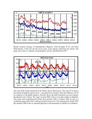
Svalgaard et al.Figure 2. Superposed epoch analysis of the average photospheric line-of-sight magnetic fieldfrom WSO keyed on sector boundaries that are Hale boundaries in the southern hemisphere,for solar cycle 21 (-,+) boundaries, 22 (+,-), and 23 (-,+). The number of boundaries (SB)and magnetograms (MG) used are as indicated. The left-hand panel shows the average signedfield, e.g. the sector structure in the photosphere. The right-hand panel shows the averagemagnitude of the field, confirming the original finding that the magnetic field is strongest atthe Hale portion of sector boundaries. Flux densities are color coded in µT.SOLA: HaleBx.tex; 21 July 2010; 7:55; p. 4

Hale Sector BoundariesFigure 3. Superposed epoch analysis of the average photospheric line-of-sight magnetic fieldfrom WSO keyed on sector boundaries that are Hale boundaries in the northern hemisphere,for solar cycle 21 (+,-) boundaries, 22 (-,+), and 23 (+,-). The number of boundaries (SB)and magnetograms (MG) used are as indicated. The left-hand panel shows the average signedfield, e.g. the sector structure in the photosphere. The right-hand panel shows the averagemagnitude of the field, confirming the original finding that the magnetic field is strongest atthe Hale portion of sector boundaries. Flux densities are color coded in µT.SOLA: HaleBx.tex; 21 July 2010; 7:55; p. 5

Svalgaard et al.Figure 4. The average magnetogram for a nominal (+,-) Hale boundary in the northernhemisphere. 910 magnetograms superposed on 765 sector boundaries for the WSO observations1976-2010. Some Data has been mirrored and sign-reversed as described in section 2.3. Thesector boundary is marked by the semi-transparent bar.To bring out the essential features of the patterns so clearly seen in Figures 2and 3 we first mirror the data in Figure 2 about the equator. We then reverse thesign of the photospheric field for magnetograms superposed on (-,+) boundaries.Finally, we construct the average of all magnetograms data so treated. Theresult (Figure 4) shows (left) what the average sector boundary looks like in thephotosphere and (right) the magnitude of the field, now for a nominal (+,-) Haleboundary.3. Evolution with Phase of the Solar CycleThe large-scale sector structure, observed in the corona and beyond, originatesfrom extended magnetic fields on both sides of a Hale boundary in the photosphere(Figure 4) where the field strength is high. This means that the sourcesof a solar sector is largely limited to one hemisphere, namely where the polaritychange matches that of the Hale polarity rule.With the large amount of data from several cycles it is possible to studyhow the structures seen in the averaged magnetograms (Figure 4) vary with thephase of the cycle. We divide a cycle into the ascending phase (first third of thecycle), maximum (second third), and declining phase (last third) and computethe averages for each in the same way as for Figure 4. The result is shown inFigure 5. The same general behavior is seen regardless of phase with the expectedvariation of field strength over the cycle: Weaker during the ascending phase,strongest at maximum, and weakest during the declining phase. The equatorwardprogression of the sector with the progress of the cycle as well as Joy’s laware clearly discernible. Note the reversal of polar field polarity.SOLA: HaleBx.tex; 21 July 2010; 7:55; p. 6

Hale Sector BoundariesFigure 5. The average magnetogram for a nominal (+,-) Hale boundary in the northernhemisphere, for three different phases of the solar cycle, in the same format as for figure 4.The color scales are identical for all three phases.SOLA: HaleBx.tex; 21 July 2010; 7:55; p. 7

Svalgaard et al.Figure 6: The average magnetogramfor a nominal (+) sectorseen ‘face on’ in the northernhemisphere. Appropriate data(WSO 1976-2010) has been mirroredand sign-reversed as describedin section 2.3. The sectorboundary is marked by thesemi-transparent bar. The semitransparentcircle encloses thearea that is mainly contributingto the Sun’s mean field also measuredat WSO (Scherrer et al.,1977).4. DiscussionThe findings of preferential photospheric magnetic fields to heliospheric magneticfield (HMF) sector structures suggests one of a number of possibilities. The mostobvious is that these photospheric structures are responsible for the HMF, andhence a correlation would simply be consistent with the Potential Field SourceSurface models (Schatten et al., 1969; Altschuler and Newkirk, 1969) wherein theHMF was seen as an extension of the solar field, as the solar wind plasma grippedthe field and extended it into the solar wind. This, however, seems insufficient toexplain our findings, since these models are symmetric, with regard to Left-Rightor East-West handedness. So, if the cause were to be a coronal phenomenon, wewould not expect the high degree of asymmetry we find.From our understanding, of the relative high abundance of field orientation(active region formation, going along with Hale’s polarity laws) relative to theHale sector boundaries we show in Figure 1 and the orientation of the subsurfacefield in accordance with, say the Babcock-Leighton dynamo models, it seems thatthe association is more deeply rooted on the Sun, than in the corona. One suchpossible explanation has recently been put forward, and although it seems to beconsistent with our findings, the author was aware of our earlier findings whenhis theory was developed, so this is not any new support for his theory.This involves a recent shallow dynamo model (Schatten, 2009), which usespercolation and clustering to accumulate magnetic flux from ephemeral regionsbelow the photosphere, where they gather together preferentially forming activeregions near the low latitudes of high toroidal magnetic flux. To understand howthis field gathering may relate to our observations, consider the following. Let usconsider a dipole field forming near one of our Hale boundaries, say as oriented inthe Northern hemisphere, as shown. Outward oriented field (ephemeral regionsgathering into sunspots) could gather such field more readily, since the Westernportion of the active region is embedded in an outward polarity background field.SOLA: HaleBx.tex; 21 July 2010; 7:55; p. 8

Hale Sector BoundariesSimilarly the Eastern portion of active regions in these environs can gather fieldpreferentially with these orientations (those orientations which are supported byHale’s laws). In other words, any little instability in this preferential orderingwould grow from pre-existing field with the orientations from their inherentenvironment.The geometry of the modern dynamo has a differing evolution than this shallowmodel: in conventional dynamo models, fields erupt from the Sun’s interioroutwards, whereas in the percolation model, field lines coalesce from small activeregions where field lines are shed from the granulations’ churning of Ephemeralregions. This temporal pattern is thus a difference between the standard dynamotheory and this new model.Aside from these differences, however, the geometry of fields at any time,in the shallow model is similar to the Babcock-Leighton field geometry (bothof course consistent with Hale’s laws), hence either view of the Solar dynamomight equally fit our observations. So, perhaps it is too early to tell whetherthe observations are preferentially supporting which theory. So, although we arefinding out some very important things about how field lines are evolving on andin the Sun, at present, it may be too early to distinguish whether the observationsprovide conclusive evidence on the exact location of the Sun’s dynamo.5. ConclusionAcknowledgementsThe authors thank Ken Schatten for fruitful discussions.SOLA: HaleBx.tex; 21 July 2010; 7:55; p. 9

Svalgaard et al.Figure 7. Schematic synoptic charts constructed by assuming a 4-sector structure and juxtaposingthe central 90 ◦ of four average magnetograms for alternating sector boundaries[(+,-)(-,+)(+,-)(-,+)] for solar cycles 21 through 23. The large-scale neutral line is sketchedusing the semi-transparent bars. The Hale-portion is marked with the brown bars. Ovals outlinethe flux concentrations of the signed solar sectors.Figure 8. As Figure 7, except showing the unsigned magnetic field. The red ovals drawattention to and confirm the finding (Svalgaard et al., 1975) that the field is at a maximum atthe Hale-portion of sector boundaries.SOLA: HaleBx.tex; 21 July 2010; 7:55; p. 10

Hale Sector BoundariesReferencesAltschuler, M.D., Newkirk, G.: 1969, Solar Phys. 9, 131Duvall, T.L.Jr., Scherrer, P.H., Svalgaard, L., Wilcox, J.M.: 1978, Solar Phys. 61, 233Echer, E., Svalgaard, L.: 2004, Geophys. Res. Lett. 31, L12808Schatten, K.H., Wilcox, J.M., Ness, N.F.: 2009, Solar Phys. 6, 442Schatten, K.H.: 2009, Solar Phys. 255, 3Scherrer, P.H., Wilcox, J.M., Svalgaard, L., Duvall, T.L.Jr., Dittmer, P.H., Gustafson, E.K.:1972, Solar Phys. 54, 353Stenflo, J.O.: 1997, http://soi.stanford.edu/science/proposals/011.stenflo/011/011.htmlSvalgaard, L.: 1973, J. Geophys. Res. 78, 2064Svalgaard, L., Wilcox, J.M.: 1975, Solar Phys. 41, 461Svalgaard, L., Wilcox, J.M., Scherrer, P.H.: 1975, Solar Phys. 45, 83Svalgaard, L., Wilcox, J.M.: 1976, Solar Phys. 49, 177Svalgaard, L., Duvall, T.L.Jr., Scherrer, P.H.: 1978, Solar Phys. 58, 225Wilcox, J.M., Svalgaard, L., Hedgecock, P.C.: 1975, J. Geophys. Res. 80, 3685Why is there an extra space before the journal names [ Astrophys. J.], except for [SolarPhys.], and also before this ‘Why’?SOLA: HaleBx.tex; 21 July 2010; 7:55; p. 11

SOLA: HaleBx.tex; 21 July 2010; 7:55; p. 12