Chapter 2 Continuous Probability Densities - DIM

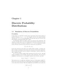
Chapter 2Continuous ProbabilityDensities2.1 Simulation of Continuous ProbabilitiesIn this section we shall show how we can use computer simulations for experimentsthat have a whole continuum of possible outcomes.ProbabilitiesExample 2.1 We begin by constructing a spinner, which consists of a circle of unitcircumference and a pointer as shown in Figure 2.1. We pick a point on the circleand label it 0, and then label every other point on the circle with the distance, sayx, from 0 to that point, measured counterclockwise. The experiment consists ofspinning the pointer and recording the label of the point at the tip of the pointer.We let the random variable X denote the value of this outcome. The sample spaceis clearly the interval [0, 1). We would like to construct a probability model in whicheach outcome is equally likely to occur.If we proceed as we did in Chapter 1 for experiments with a finite number ofpossible outcomes, then we must assign the probability 0 to each outcome, sinceotherwise, the sum of the probabilities, over all of the possible outcomes, wouldnot equal 1. (In fact, summing an uncountable number of real numbers is a trickybusiness; in particular, in order for such a sum to have any meaning, at mostcountably many of the summands can be different than 0.) However, if all of theassigned probabilities are 0, then the sum is 0, not 1, as it should be.In the next section, we will show how to construct a probability model in thissituation. At present, we will assume that such a model can be constructed. Wewill also assume that in this model, if E is an arc of the circle, and E is of lengthp, then the model will assign the probability p to E. This means that if the pointeris spun, the probability that it ends up pointing to a point in E equals p, which iscertainly a reasonable thing to expect.41

42 CHAPTER 2. CONTINUOUS PROBABILITY DENSITIESx0Figure 2.1: A spinner.To simulate this experiment on a computer is an easy matter. Many computersoftware packages have a function which returns a random real number in the interval[0, 1]. Actually, the returned value is always a rational number, and thevalues are determined by an algorithm, so a sequence of such values is not trulyrandom. Nevertheless, the sequences produced by such algorithms behave muchlike theoretically random sequences, so we can use such sequences in the simulationof experiments. On occasion, we will need to refer to such a function. We will callthis function rnd.✷Monte Carlo Procedure and AreasIt is sometimes desirable to estimate quantities whose exact values are difficult orimpossible to calculate exactly. In some of these cases, a procedure involving chance,called a Monte Carlo procedure, can be used to provide such an estimate.Example 2.2 In this example we show how simulation can be used to estimateareas of plane figures. Suppose that we program our computer to provide a pair(x, y) or numbers, each chosen independently at random from the interval [0, 1].Then we can interpret this pair (x, y) as the coordinates of a point chosen at randomfrom the unit square. Events are subsets of the unit square. Our experience withExample 2.1 suggests that the point is equally likely to fall in subsets of equal area.Since the total area of the square is 1, the probability of the point falling in a specificsubset E of the unit square should be equal to its area. Thus, we can estimate thearea of any subset of the unit square by estimating the probability that a pointchosen at random from this square falls in the subset.We can use this method to estimate the area of the region E under the curvey = x 2 in the unit square (see Figure 2.2). We choose a large number of points (x, y)at random and record what fraction of them fall in the region E = { (x, y) :y≤x 2 }.The program MonteCarlo will carry out this experiment for us. Running thisprogram for 10,000 experiments gives an estimate of .325 (see Figure 2.3).From these experiments we would estimate the area to be about 1/3. Of course,

2.1. SIMULATION OF CONTINUOUS PROBABILITIES 43y1y = x 2E1xFigure 2.2: Area under y = x 2 .for this simple region we can find the exact area by calculus. In fact,Area of E =∫ 10x 2 dx = 1 3 .We have remarked in Chapter 1 that, when we simulate an experiment of this typen times to estimate a probability, we can expect the answer to be in error by atmost 1/ √ n at least 95 percent of the time. For 10,000 experiments we can expectan accuracy of 0.01, and our simulation did achieve this accuracy.This same argument works for any region E of the unit square. For example,suppose E is the circle with center (1/2, 1/2) and radius 1/2. Then the probabilitythat our random point (x, y) lies inside the circle is equal to the area of the circle,that is,( 1P (E) =π =2)2 π 4 .If we did not know the value of π, we could estimate the value by performing thisexperiment a large number of times!✷The above example is not the only way of estimating the value of π by a chanceexperiment. Here is another way, discovered by Buffon. 11 G. L. Buffon, in “Essai d’Arithmétique Morale,” Oeuvres Complètes de Buffon avec Supplements,tome iv, ed. Duménil (Paris, 1836).

44 CHAPTER 2. CONTINUOUS PROBABILITY DENSITIES11000 trialsy = x 2EEstimate of area is .3251Figure 2.3: Computing the area by simulation.Buffon’s NeedleExample 2.3 Suppose that we take a card table and draw across the top surfacea set of parallel lines a unit distance apart. We then drop a common needle ofunit length at random on this surface and observe whether or not the needle liesacross one of the lines. We can describe the possible outcomes of this experimentby coordinates as follows: Let d be the distance from the center of the needle to thenearest line. Next, let L be the line determined by the needle, and define θ as theacute angle that the line L makes with the set of parallel lines. (The reader shouldcertainly be wary of this description of the sample space. We are attempting tocoordinatize a set of line segments. To see why one must be careful in the choiceof coordinates, see Example 2.6.) Using this description, we have 0 ≤ d ≤ 1/2, and0 ≤ θ ≤ π/2. Moreover, we see that the needle lies across the nearest line if andonly if the hypotenuse of the triangle (see Figure 2.4) is less than half the length ofthe needle, that is,dsin θ < 1 2 .Now we assume that when the needle drops, the pair (θ, d) is chosen at randomfrom the rectangle 0 ≤ θ ≤ π/2, 0 ≤ d ≤ 1/2. We observe whether the needle liesacross the nearest line (i.e., whether d ≤ (1/2) sin θ). The probability of this eventE is the fraction of the area of the rectangle which lies inside E (see Figure 2.5).

2.1. SIMULATION OF CONTINUOUS PROBABILITIES 451/2θdFigure 2.4: Buffon’s experiment.d1/2E00π/2θFigure 2.5: Set E of pairs (θ, d) with d< 1 2sin θ.Now the area of the rectangle is π/4, while the area of E isHence, we getArea =∫ π/2012 sin θdθ= 1 2 .P (E) = 1/2π/4 = 2 π .The program BuffonsNeedle simulates this experiment. In Figure 2.6, we showthe position of every 100th needle in a run of the program in which 10,000 needleswere “dropped.” Our final estimate for π is 3.139. While this was within 0.003 ofthe true value for π we had no right to expect such accuracy. The reason for thisis that our simulation estimates P (E). While we can expect this estimate to be inerror by at most 0.001, a small error in P (E) gets magnified when we use this tocompute π =2/P (E). Perlman and Wichura, in their article “Sharpening Buffon’s

46 CHAPTER 2. CONTINUOUS PROBABILITY DENSITIES5.00100004.504.003.503.003.1392.502.001.501.000.500.00Figure 2.6: Simulation of Buffon’s needle experiment.Needle,” 2 show that we can expect to have an error of not more than 5/ √ n about95 percent of the time. Here n is the number of needles dropped. Thus for 10,000needles we should expect an error of no more than 0.05, and that was the case here.We see that a large number of experiments is necessary to get a decent estimate forπ. ✷In each of our examples so far, events of the same size are equally likely. Hereis an example where they are not. We will see many other such examples later.Example 2.4 Suppose that we choose two random real numbers in [0, 1] and addthem together. Let X be the sum. How is X distributed?To help understand the answer to this question, we can use the program Areabargraph.This program produces a bar graph with the property that on eachinterval, the area, rather than the height, of the bar is equal to the fraction of outcomesthat fell in the corresponding interval. We have carried out this experiment1000 times; the data is shown in Figure 2.7. It appears that the function definedby{x, if 0 ≤ x ≤ 1,f(x) =2 − x, if 1

2.1. SIMULATION OF CONTINUOUS PROBABILITIES 4710.80.60.40.200 0.5 1 1.5 2Figure 2.7: Sum of two random numbers.[a, b] approximates the probability that a ≤ X ≤ b. But the sum of the areas ofthese bars also approximates the integral∫ baf(x) dx .This suggests that for an experiment with a continuum of possible outcomes, if wefind a function with the above property, then we will be able to use it to calculateprobabilities. In the next section, we will show how to determine the functionf(x).✷Example 2.5 Suppose that we choose 100 random numbers in [0, 1], and let Xrepresent their sum. How is X distributed? We have carried out this experiment10000 times; the results are shown in Figure 2.8. It is not so clear what functionfits the bars in this case. It turns out that the type of function which does the jobis called a normal density function. This type of function is sometimes referred toas a “bell-shaped” curve. It is among the most important functions in the subjectof probability, and will be formally defined in Section 5.2 of Chapter . ✷Our last example explores the fundamental question of how probabilities areassigned.Bertrand’s ParadoxExample 2.6 A chord of a circle is a line segment both of whose endpoints lie onthe circle. Suppose that a chord is drawn at random in a unit circle. What is theprobability that its length exceeds √ 3?Our answer will depend on what we mean by random, which will depend, in turn,on what we choose for coordinates. The sample space Ω is the set of all possiblechords in the circle. To find coordinates for these chords, we first introduce a

48 CHAPTER 2. CONTINUOUS PROBABILITY DENSITIES0.140.120.10.080.060.040.02040 45 50 55 60Figure 2.8: Sum of 100 random numbers.yAMBαθβxFigure 2.9: Random chord.rectangular coordinate system with origin at the center of the circle (see Figure 2.9).We note that a chord of a circle is perpendicular to the radial line containing themidpoint of the chord. We can describe each chord by giving:1. The rectangular coordinates (x, y) of the midpoint M, or2. The polar coordinates (r, θ) of the midpoint M, or3. The polar coordinates (1,α) and (1,β) of the endpoints A and B.In each case we shall interpret at random to mean: choose these coordinates atrandom.We can easily estimate this probability by computer simulation. In programmingthis simulation, it is convenient to include certain simplifications, which we describein turn:

2.1. SIMULATION OF CONTINUOUS PROBABILITIES 491. To simulate this case, we choose values for x and y from [−1, 1] at random.Then we check whether x 2 + y 2 ≤ 1. If not, the point M =(x, y) lies outsidethe circle and cannot be the midpoint of any chord, and we ignore it. Otherwise,M lies inside the circle and is the midpoint of a unique chord, whoselength L is given by the formula:L =2 √ 1−(x 2 +y 2 ).2. To simulate this case, we take account of the fact that any rotation of thecircle does not change the length of the chord, so we might as well assume inadvance that the chord is horizontal. Then we choose r from [−1, 1] at random,and compute the length of the resulting chord with midpoint (r, π/2) by theformula:L =2 √ 1−r 2 .3. To simulate this case, we assume that one endpoint, say B, lies at (1, 0) (i.e.,that β = 0). Then we choose a value for α from [0, 2π] at random and computethe length of the resulting chord, using the Law of Cosines, by the formula:L = √ 2 − 2 cos α.The program BertrandsParadox carries out this simulation. Running thisprogram produces the results shown in Figure 2.10. In the first circle in this figure,a smaller circle has been drawn. Those chords which intersect this smaller circlehave length at least √ 3. In the second circle in the figure, the vertical line intersectsall chords of length at least √ 3. In the third circle, again the vertical line intersectsall chords of length at least √ 3.In each case we run the experiment a large number of times and record thefraction of these lengths that exceed √ 3. We have printed the results of every100th trial up to 10,000 trials.It is interesting to observe that these fractions are not the same in the three cases;they depend on our choice of coordinates. This phenomenon was first observed byBertrand, and is now known as Bertrand’s paradox. 3 It is actually not a paradox atall; it is merely a reflection of the fact that different choices of coordinates will leadto different assignments of probabilities. Which assignment is “correct” depends onwhat application or interpretation of the model one has in mind.One can imagine a real experiment involving throwing long straws at a circledrawn on a card table. A “correct” assignment of coordinates should not dependon where the circle lies on the card table, or where the card table sits in the room.Jaynes 4 has shown that the only assignment which meets this requirement is (2).In this sense, the assignment (2) is the natural, or “correct” one (see Exercise 11).√We can easily see in each case what the true probabilities are if we note that3 is the length of the side of an inscribed equilateral triangle. Hence, a chord has3 J. Bertrand, Calcul des Probabilités (Paris: Gauthier-Villars, 1889).4 E. T. Jaynes, “The Well-Posed Problem,” in Papers on Probability, Statistics and StatisticalPhysics, R. D. Rosencrantz, ed. (Dordrecht: D. Reidel, 1983), pp. 133–148.

50 CHAPTER 2. CONTINUOUS PROBABILITY DENSITIES10000 10000 100001.0.9.8.7.6.5.4.2.3 .227.1.01.0.9.8.7.6.5.4.2.3.1.0.4881.0.9.8.7.6.5.4.2.3.1.0.332Figure 2.10: Bertrand’s paradox.length L> √ 3 if its midpoint has distance d √ 3ineachofthethree cases.1. L> √ 3 if(x, y) lies inside a circle of radius 1/2, which occurs with probabilityp = π(1/2)2π(1) 2 = 1 4 .2. L> √ 3if|r| √ 3if2π/3

2.1. SIMULATION OF CONTINUOUS PROBABILITIES 51Length of Number of Number of EstimateExperimenter needle casts crossings for πWolf, 1850 .8 5000 2532 3.1596Smith, 1855 .6 3204 1218.5 3.1553De Morgan, c.1860 1.0 600 382.5 3.137Fox, 1864 .75 1030 489 3.1595Lazzerini, 1901 .83 3408 1808 3.1415929Reina, 1925 .5419 2520 869 3.1795Table 2.1: Buffon needle experiments to estimate π.presented a number of mortality tables and used them to compute, for each agegroup, the expected remaining lifetime. From his table he observed: the expectedremaining lifetime of an infant of one year is 33 years, while that of a man of 21years is also approximately 33 years. Thus, a father who is not yet 21 can hope tolive longer than his one year old son, but if the father is 40, the odds are already 3to 2 that his son will outlive him. 6Buffon wanted to show that not all probability calculations rely only on algebra,but that some rely on geometrical calculations. One such problem was his famous“needle problem” as discussed in this chapter. 7 In his original formulation, Buffondescribes a game in which two gamblers drop a loaf of French bread on a wide-boardfloor and bet on whether or not the loaf falls across a crack in the floor. Buffonasked: what length L should the bread loaf be, relative to the width W of thefloorboards, so that the game is fair. He found the correct answer (L =(π/4)W )using essentially the methods described in this chapter. He also considered the caseof a checkerboard floor, but gave the wrong answer in this case. The correct answerwas given later by Laplace.The literature contains descriptions of a number of experiments that were actuallycarried out to estimate π by this method of dropping needles. N. T. Gridgeman 8discusses the experiments shown in Table 2.1. (The halves for the number of crossingcomes from a compromise when it could not be decided if a crossing had actuallyoccurred.) He observes, as we have, that 10,000 casts could do no more than establishthe first decimal place of π with reasonable confidence. Gridgeman points outthat, although none of the experiments used even 10,000 casts, they are surprisinglygood, and in some cases, too good. The fact that the number of casts is not alwaysa round number would suggest that the authors might have resorted to clever stoppingto get a good answer. Gridgeman comments that Lazzerini’s estimate turnedout to agree with a well-known approximation to π, 355/113=3.1415929, discoveredby the fifth-century Chinese mathematician, Tsu Ch’ungchih. Gridgeman saysthat he did not have Lazzerini’s original report, and while waiting for it (knowing6 G. L. Buffon, “Essai d’Arithmétique Morale,” p. 301.7 ibid., pp. 277–278.8 N. T. Gridgeman, “Geometric Probability and the Number π” Scripta Mathematika, vol. 25,no. 3, (1960), pp. 183–195.

52 CHAPTER 2. CONTINUOUS PROBABILITY DENSITIESonly the needle crossed a line 1808 times in 3408 casts) deduced that the length ofthe needle must have been 5/6. He calculated this from Buffon’s formula, assumingπ = 355/113:L = πP(E)2= 1 2( 355113)( ) 1808= 5 3408 6 = .8333 .Even with careful planning one would have to be extremely lucky to be able to stopso cleverly.The second author likes to trace his interest in probability theory to the ChicagoWorld’s Fair of 1933 where he observed a mechanical device dropping needles anddisplaying the ever-changing estimates for the value of π. (The first author likes totrace his interest in probability theory to the second author.)Exercises*1 In the spinner problem (see Example 2.1) divide the unit circumference intothree arcs of length 1/2, 1/3, and 1/6. Write a program to simulate thespinner experiment 1000 times and print out what fraction of the outcomesfall in each of the three arcs. Now plot a bar graph whose bars have width 1/2,1/3, and 1/6, and areas equal to the corresponding fractions as determinedby your simulation. Show that the heights of the bars are all nearly the same.2 Do the same as in Exercise 1, but divide the unit circumference into five arcsof length 1/3, 1/4, 1/5, 1/6, and 1/20.3 Alter the program MonteCarlo to estimate the area of the circle of radius1/2 with center at (1/2, 1/2) inside the unit square by choosing 1000 pointsat random. Compare your results with the true value of π/4. Use your resultsto estimate the value of π. How accurate is your estimate?4 Alter the program MonteCarlo to estimate the area under the graph ofy = sin πx inside the unit square by choosing 10,000 points at random. Nowcalculate the true value of this area and use your results to estimate the valueof π. How accurate is your estimate?5 Alter the program MonteCarlo to estimate the area under the graph ofy =1/(x+ 1) in the unit square in the same way as in Exercise 4. Calculatethe true value of this area and use your simulation results to estimate thevalue of log 2. How accurate is your estimate?6 To simulate the Buffon’s needle problem we choose independently the distanced and the angle θ at random, with 0 ≤ d ≤ 1/2 and 0 ≤ θ ≤ π/2,and check whether d ≤ (1/2) sin θ. Doing this a large number of times, weestimate π as 2/a, where a is the fraction of the times that d ≤ (1/2) sin θ.Write a program to estimate π by this method. Run your program severaltimes for each of 100, 1000, and 10,000 experiments. Does the accuracy ofthe experimental approximation for π improve as the number of experimentsincreases?

2.1. SIMULATION OF CONTINUOUS PROBABILITIES 537 For Buffon’s needle problem, Laplace 9 considered a grid with horizontal andvertical lines one unit apart. He showed that the probability that a needle oflength L ≤ 1 crosses at least one line is4L − L2p = .πTo simulate this experiment we choose at random an angle θ between 0 andπ/2 and independently two numbers d 1 and d 2 between 0 and L/2. (The twonumbers represent the distance from the center of the needle to the nearesthorizontal and vertical line.) The needle crosses a line if either d 1 ≤ (L/2) sin θor d ≤ (L/2) cos θ. We do this a large number of times and estimate π as4L − L2¯π = ,awhere a is the proportion of times that the needle crosses at least one line.Write a program to estimate π by this method, run your program for 100,1000, and 10,000 experiments, and compare your results with Buffon’s methoddescribed in Exercise 6. (Take L = 1.)8 A long needle of length L much bigger than 1 is dropped on a grid withhorizontal and vertical lines one unit apart. We will see (in Exercise 6.3.28)that the average number a of lines crossed is approximatelya = 4L π .To estimate π by simulation, pick an angle θ at random between 0 and π/2 andcompute L sin θ + L cos θ. This may be used for the number of lines crossed.Repeat this many times and estimate π by¯π = 4L a ,where a is the average number of lines crossed per experiment. Write a programto simulate this experiment and run your program for the number ofexperiments equal to 100, 1000, and 10,000. Compare your results with themethods of Laplace or Buffon for the same number of experiments. (UseL = 100.)The following exercises involve experiments in which not all outcomes areequally likely. We shall consider such experiments in detail in the next section,but we invite you to explore a few simple cases here.9 A large number of waiting time problems have an exponential distribution ofoutcomes. We shall see (in Section 5.2) that such outcomes are simulated bycomputing (−1/λ) log(rnd), where λ>0. For waiting times produced in thisway, the average waiting time is 1/λ. For example, the times spent waiting for9 P. S. Laplace, Théorie Analytique des Probabilités (Paris: Courcier, 1812).

54 CHAPTER 2. CONTINUOUS PROBABILITY DENSITIESa car to pass on a highway, or the times between emissions of particles froma radioactive source, are simulated by a sequence of random numbers, eachof which is chosen by computing −λ log(rnd), where 1/λ is the average timebetween cars or emissions. Write a program to simulate the times betweencars when the average time between cars is 30 seconds. Have your programcompute an area bar graph for these times by breaking the time interval from0 to 120 into 24 subintervals. On the same pair of axes, plot the functionf(x) =(1/30)e −(1/30)x . Does the function fit the bar graph well?10 In Exercise 9, the distribution came “out of a hat.” In this problem, we willagain consider an experiment whose outcomes are not equally likely. We willdetermine a function f(x) which can be used to determine the probability ofcertain events. Let T be the right triangle in the plane with vertices at thepoints (0, 0), (1, 0), and (0, 1). The experiment consists of picking a pointat random in the interior of T , and recording only the x-coordinate of thepoint. Thus, the sample space is the set [0, 1], but the outcomes do not seemto be equally likely. We can simulate this experiment by asking a computer toreturn two random real numbers in [0, 1], and recording the first of these twonumbers if their sum is less than 1. Write this program and run it for 10,000trials. Then make a bar graph of the result, breaking the interval [0, 1] into10 intervals. Compare the bar graph with the function f(x) =.2−.2x.Nowshow that there is a constant c such that the height of T at the x-coordinatevalue x is c times f(x) for every x in [0, 1]. Finally, show that∫ 10f(x) dx =1.How might one use the function f(x) to determine the probability that theoutcome is between .2 and .5?11 Here is another way to pick a chord at random on the circle of unit radius.Imagine that we have a card table whose sides are of length 100. We placecoordinate axes on the table in such a way that each side of the table is parallelto one of the axes, and so that the center of the table is the origin. We nowplace a circle of unit radius on the table so that the center of the circle is theorigin. Now pick out a point (x 0 ,y 0 ) at random in the square, and an angle θat random in the interval (−π/2,π/2). Let m = tan θ. Then the equation ofthe line passing through (x 0 ,y 0 ) with slope m isy = y 0 + m(x − x 0 ) ,and the distance of this line from the center of the circle (i.e., the origin) isd =y 0 − mx 0∣ √ m2 +1∣ .We can use this distance formula to check whether the line intersects the circle(i.e., whether d

2.2. CONTINUOUS DENSITY FUNCTIONS 55This describes an experiment of dropping a long straw at random on a tableon which a circle is drawn.Write a program to simulate this experiment 10000 times and estimate theprobability that the length of the chord is greater than √ 3. How does yourestimate compare with the results of Example 2.6?2.2 Continuous Density FunctionsIn the previous section we have seen how to simulate experiments with a wholecontinuum of possible outcomes and have gained some experience in thinking aboutsuch experiments. Now we turn to the general problem of assigning probabilities tothe outcomes and events in such experiments. We shall restrict our attention hereto those experiments whose sample space can be taken as a suitably chosen subsetof the line, the plane, or some other Euclidean space. We begin with some simpleexamples.SpinnersExample 2.7 The spinner experiment described in Example 2.1 has the interval[0, 1) as the set of possible outcomes. We would like to construct a probabilitymodel in which each outcome is equally likely to occur. We saw that in such amodel, it is necessary to assign the probability 0 to each outcome. This does not atall mean that the probability of every event must be zero. On the contrary, if welet the random variable X denote the outcome, then the probabilityP (0≤X ≤1)that the head of the spinner comes to rest somewhere in the circle, should be equalto 1. Also, the probability that it comes to rest in the upper half of the circle shouldbe the same as for the lower half, so that(P 0 ≤ X< 1 ) ( )1=P2 2 ≤X

56 CHAPTER 2. CONTINUOUS PROBABILITY DENSITIES10.80.60.40.200 0.2 0.4 0.6 0.8 1Figure 2.11: Spinner experiment.The difference is that in the continuous case, the quantity being integrated, f(x),is not the probability of the outcome x. (However, if one uses infinitesimals, onecan consider f(x) dx as the probability of the outcome x.)In the continuous case, we will use the following convention. If the set of outcomesis a set of real numbers, then the individual outcomes will be referred toby small Roman letters such as x. If the set of outcomes is a subset of R 2 , thenthe individual outcomes will be denoted by (x, y). In either case, it may be moreconvenient to refer to an individual outcome by using ω, as in Chapter 1.Figure 2.11 shows the results of 1000 spins of the spinner. The function f(x)is also shown in the figure. The reader will note that the area under f(x) andabove a given interval is approximately equal to the fraction of outcomes that fellin that interval. The function f(x) is called the density function of the randomvariable X. The fact that the area under f(x) and above an interval correspondsto a probability is the defining property of density functions. A precise definitionof density functions will be given shortly.✷DartsExample 2.8 A game of darts involves throwing a dart at a circular target of unitradius. Suppose we throw a dart once so that it hits the target, and we observewhere it lands.To describe the possible outcomes of this experiment, it is natural to take as oursample space the set Ω of all the points in the target. It is convenient to describethese points by their rectangular coordinates, relative to a coordinate system withorigin at the center of the target, so that each pair (x, y) of coordinates with x 2 +y 2 ≤1 describes a possible outcome of the experiment. Then Ω = { (x, y) :x 2 +y 2 ≤1}is a subset of the Euclidean plane, and the event E = { (x, y) :y>0}, for example,corresponds to the statement that the dart lands in the upper half of the target,and so forth. Unless there is reason to believe otherwise (and with experts at the

2.2. CONTINUOUS DENSITY FUNCTIONS 57game there may well be!), it is natural to assume that the coordinates are chosenat random. (When doing this with a computer, each coordinate is chosen uniformlyfrom the interval [−1, 1]. If the resulting point does not lie inside the unit circle,the point is not counted.) Then the arguments used in the preceding example showthat the probability of any elementary event, consisting of a single outcome, mustbe zero, and suggest that the probability of the event that the dart lands in anysubset E of the target should be determined by what fraction of the target area liesin E. Thus,area of E area of EP (E) == .area of target πThis can be written in the form∫P (E) = f(x)dx ,Ewhere f(x) is the constant function with value 1/π. In particular, if E = { (x, y) :x 2 +y 2 ≤a 2 }is the event that the dart lands within distance a

58 CHAPTER 2. CONTINUOUS PROBABILITY DENSITIES21.51.510.500 0.2 0.4 0.6 0.8 1Figure 2.12: Distribution of dart distances in 400 throws.Thus, P (E) =2(length of E)(midpoint of E). Here we see that the probabilityassigned to the interval E depends not only on its length but also on its midpoint(i.e., not only on how long it is, but also on where it is). Roughly speaking, in thisexperiment, events of the form E =[a, b] are more likely if they are near the rimof the target and less likely if they are near the center. (A common experience forbeginners! The conclusion might well be different if the beginner is replaced by anexpert.)Again we can simulate this by computer. We divide the target area into tenconcentric regions of equal thickness.The computer program Darts throws n darts and records what fraction of thetotal falls in each of these concentric regions. The program Areabargraph thenplots a bar graph with the area of the ith bar equal to the fraction of the totalfalling in the ith region. Running the program for 1000 darts resulted in the bargraph of Figure 2.12.Note that here the heights of the bars are not all equal, but grow approximatelylinearly with r. In fact, the linear function y =2rappears to fit our bar graph quitewell. This suggests that the probability that the dart falls within a distance a of thecenter should be given by the area under the graph of the function y =2rbetween0 and a. This area is a 2 , which agrees with the probability we have assigned aboveto this event.✷Sample Space CoordinatesThese examples suggest that for continuous experiments of this sort we should assignprobabilities for the outcomes to fall in a given interval by means of the area undera suitable function.More generally, we suppose that suitable coordinates can be introduced into thesample space Ω, so that we can regard Ω as a subset of R n . We call such a samplespace a continuous sample space. We let X be a random variable which representsthe outcome of the experiment. Such a random variable is called a continuousrandom variable. We then define a density function for X as follows.

2.2. CONTINUOUS DENSITY FUNCTIONS 59Density Functions of Continuous Random VariablesDefinition 2.1 Let X be a continuous real-valued random variable.function for X is a real-valued function f which satisfiesP (a ≤ X ≤ b) =for all a, b ∈ R.∫ baf(x)dxA density✷We note that it is not the case that all continuous real-valued random variablespossess density functions. However, in this book, we will only consider continuousrandom variables for which density functions exist.In terms of the density f(x), if E is a subset of R, then∫P (X ∈ E) = f(x)dx .The notation here assumes that E is a subset of R for which ∫ f(x) dx makesEsense.Example 2.10 (Example 2.7 continued) In the spinner experiment, we choose forour set of outcomes the interval 0 ≤ x

60 CHAPTER 2. CONTINUOUS PROBABILITY DENSITIESIn these two examples, the density function is constant and does not dependon the particular outcome. It is often the case that experiments in which thecoordinates are chosen at random can be described by constant density functions,and, as in Section 1.2, we call such density functions uniform or equiprobable. Notall experiments are of this type, however.Example 2.12 (Example 2.9 continued) In the second dart game experiment, wechoose for our sample space the unit interval on the real line and for our densitythe function{2r, if 0

2.2. CONTINUOUS DENSITY FUNCTIONS 61A glance at the graph of a density function tells us immediately which events ofan experiment are more likely. Roughly speaking, we can say that where the densityis large the events are more likely, and where it is small the events are less likely.In Example 2.4 the density function is largest at 1. Thus, given the two intervals[0,a] and [1, 1+a], where a is a small positive real number, we see that X is morelikely to take on a value in the second interval than in the first.Cumulative Distribution Functions of Continuous RandomVariablesWe have seen that density functions are useful when considering continuous randomvariables. There is another kind of function, closely related to these densityfunctions, which is also of great importance. These functions are called cumulativedistribution functions.Definition 2.2 Let X be a continuous real-valued random variable.cumulative distribution function of X is defined by the equationThen theF X (x) =P(X≤x).If X is a continuous real-valued random variable which possesses a density function,then it also has a cumulative distribution function, and the following theorem showsthat the two functions are related in a very nice way.Theorem 2.1 Let X be a continuous real-valued random variable with densityfunction f(x). Then the function defined byF (x) =∫ x−∞f(t) dtis the cumulative distribution function of X. Furthermore, we havedF (x) =f(x).dx✷Proof. By definition,Let E =(−∞,x]. Thenwhich equalsF (x) =P(X≤x).P (X ≤ x) =P(X∈E),∫ x−∞f(t) dt .Applying the Fundamental Theorem of Calculus to the first equation in thestatement of the theorem yields the second statement.✷

62 CHAPTER 2. CONTINUOUS PROBABILITY DENSITIES21.751.5f (x)X1.251F (x)X0.750.50.25-1 -0.5 0 0.5 1 1.5 2Figure 2.13: Distribution and density for X = U 2 .In many experiments, the density function of the relevant random variable is easyto write down. However, it is quite often the case that the cumulative distributionfunction is easier to obtain than the density function. (Of course, once we havethe cumulative distribution function, the density function can easily be obtained bydifferentiation, as the above theorem shows.) We now give some examples whichexhibit this phenomenon.Example 2.13 A real number is chosen at random from [0, 1] with uniform probability,and then this number is squared. Let X represent the result. What is thecumulative distribution function of X? What is the density of X?We begin by letting U represent the chosen real number. Then X = U 2 . If0 ≤ x ≤ 1, then we haveF X (x) = P(X ≤ x)= P(U 2 ≤ x)= P(U ≤ √ x)= √ x.It is clear that X always takes on a value between 0 and 1, so the cumulativedistribution function of X is given by⎧⎨ 0,√if x ≤ 0,F X (x) = x, if 0 ≤ x ≤ 1,⎩1, if x ≥ 1.From this we easily calculate that the density function of X is⎧⎨ 0, if x ≤ 0,f X (x) = 1/(2 √ x), if 0 ≤ x ≤ 1,⎩0, if x>1.Note that F X (x) is continuous, but f X (x) is not. (See Figure 2.13.)✷

2.2. CONTINUOUS DENSITY FUNCTIONS 6310.80.60.40.2E .80.2 0.4 0.6 0.8 1Figure 2.14: Calculation of distribution function for Example 2.14.When referring to a continuous random variable X (say with a uniform densityfunction), it is customary to say that “X is uniformly distributed on the interval[a, b].” It is also customary to refer to the cumulative distribution function of X asthe distribution function of X. Thus, the word “distribution” is being used in severaldifferent ways in the subject of probability. (Recall that it also has a meaningwhen discussing discrete random variables.) When referring to the cumulative distributionfunction of a continuous random variable X, we will always use the word“cumulative” as a modifier, unless the use of another modifier, such as “normal” or“exponential,” makes it clear. Since the phrase “uniformly densitied on the interval[a, b]” is not acceptable English, we will have to say “uniformly distributed” instead.Example 2.14 In Example 2.4, we considered a random variable, defined to bethe sum of two random real numbers chosen uniformly from [0, 1]. Let the randomvariables X and Y denote the two chosen real numbers. Define Z = X + Y . Wewill now derive expressions for the cumulative distribution function and the densityfunction of Z.Here we take for our sample space Ω the unit square in R 2 with uniform density.A point ω ∈ Ω then consists of a pair (x, y) of numbers chosen at random. Then0 ≤ Z ≤ 2. Let E z denote the event that Z ≤ z. In Figure 2.14, we show the setE .8 . The event E z , for any z between 0 and 1, looks very similar to the shaded setin the figure. For 1

64 CHAPTER 2. CONTINUOUS PROBABILITY DENSITIES1F Z(z)10.80.60.80.6f (z)Z0.40.40.20.2-1 1 2 3-1 1 2 3Figure 2.15: Distribution and density functions for Example 2.14.E1ZFigure 2.16: Calculation of F z for Example 2.15.=⎧⎪⎨⎪⎩0, if z

2.2. CONTINUOUS DENSITY FUNCTIONS 6521F (z)Z1.751.5f (z)Z0.81.250.610.40.750.50.20.25-1 -0.5 0.5 1 1.5 2-1 -0.5 0 0.5 1 1.5 2Figure 2.17: Distribution and density for Z = √ X 2 + Y 2 .E be the event {Z ≤ z}. Then the distribution function F Z of Z (see Figure 2.16)is given byF Z (z) = P(Z ≤ z)=Area of EArea of target .Thus, we easily compute that⎧⎨ 0, if z ≤ 0,F Z (z) = z 2 , if 0 ≤ z ≤ 1,⎩1, if z>1.The density f Z (z) is given again by the derivative of F Z (z):⎧⎨ 0, if z ≤ 0,f Z (z) = 2z, if 0 ≤ z ≤ 1,⎩0, if z>1.The reader is referred to Figure 2.17 for the graphs of these functions.We can verify this result by simulation, as follows: We choose values for X andY at random from [0, 1] with uniform distribution, calculate Z = √ X 2 + Y 2 , checkwhether 0 ≤ Z ≤ 1, and present the results in a bar graph (see Figure 2.18). ✷Example 2.16 Suppose Mr. and Mrs. Lockhorn agree to meet at the Hanover Innbetween 5:00 and 6:00 P.M. on Tuesday. Suppose each arrives at a time between5:00 and 6:00 chosen at random with uniform probability. What is the distributionfunction for the length of time that the first to arrive has to wait for the other?What is the density function?Here again we can take the unit square to represent the sample space, and (X, Y )as the arrival times (after 5:00 P.M.) for the Lockhorns. Let Z = |X − Y |. Then wehave F X (x) =xand F Y (y) =y. Moreover (see Figure 2.19),F Z (z) = P(Z ≤ z)= P(|X −Y|≤z)= Area of E.

66 CHAPTER 2. CONTINUOUS PROBABILITY DENSITIES21.510.500 0.2 0.4 0.6 0.8 1Figure 2.18: Simulation results for Example 2.15.Thus, we have⎧⎨ 0, if z ≤ 0,F Z (z) = 1 − (1 − z) 2 , if 0 ≤ z ≤ 1,⎩1, if z>1.The density f Z (z) is again obtained by differentiation:⎧⎨ 0, if z ≤ 0,f Z (z) = 2(1 − z), if 0 ≤ z ≤ 1,⎩0, if z>1.✷Example 2.17 There are many occasions where we observe a sequence of occurrenceswhich occur at “random” times. For example, we might be observing emissionsof a radioactive isotope, or cars passing a milepost on a highway, or light bulbsburning out. In such cases, we might define a random variable X to denote the timebetween successive occurrences. Clearly, X is a continuous random variable whoserange consists of the non-negative real numbers. It is often the case that we canmodel X by using the exponential density. This density is given by the formula{λef(t) =−λt , if t ≥ 0,0, if t

2.2. CONTINUOUS DENSITY FUNCTIONS 671 - z1 - zE1 - z1 - zFigure 2.19: Calculation of F Z .0.030.0250.02f (t) = (1/30) e - (1/30) t0.0150.010.00520 40 60 80 100 120Figure 2.20: Exponential density with λ =1/30.

68 CHAPTER 2. CONTINUOUS PROBABILITY DENSITIES0.030.0250.020.0150.010.00500 20 40 60 80 100Figure 2.21: Residual lifespan of a hard drive.is distributed according to the exponential density. We will assume that this modelapplies here, with λ =1/30.Now suppose that we have been operating our computer for 15 months. Weassume that the original hard drive is still running. We ask how long we shouldexpect the hard drive to continue to run. One could reasonably expect that thehard drive will run, on the average, another 15 months. (One might also guessthat it will run more than 15 months, since the fact that it has already run for 15months implies that we don’t have a lemon.) The time which we have to wait isa new random variable, which we will call Y . Obviously, Y = X − 15. We canwrite a computer program to produce a sequence of simulated Y -values. To do this,we first produce a sequence of X’s, and discard those values which are less thanor equal to 15 (these values correspond to the cases where the hard drive has quitrunning before 15 months). To simulate a value of X, we compute the value of theexpression(− 1 )log(rnd) ,λwhere rnd represents a random real number between 0 and 1. (That this expressionhas the exponential density will be shown in Chapter .) Figure 2.21 shows an areabar graph of 10,000 simulated Y -values.The average value of Y in this simulation is 29.74, which is closer to the originalaverage life span of 30 months than to the value of 15 months which was guessedabove. Also, the distribution of Y is seen to be close to the distribution of X.It is in fact the case that X and Y have the same distribution. This property iscalled the memoryless property, because the amount of time that we have to waitfor an occurrence does not depend on how long we have already waited. The onlycontinuous density function with this property is the exponential density. ✷

2.2. CONTINUOUS DENSITY FUNCTIONS 69Assignment of ProbabilitiesA fundamental question in practice is: How shall we choose the probability densityfunction in describing any given experiment? The answer depends to a great extenton the amount and kind of information available to us about the experiment. Insome cases, we can see that the outcomes are equally likely. In some cases, we cansee that the experiment resembles another already described by a known density.In some cases, we can run the experiment a large number of times and make areasonable guess at the density on the basis of the observed distribution of outcomes,as we did in Chapter 1. In general, the problem of choosing the right density functionfor a given experiment is a central problem for the experimenter and is not alwayseasy to solve (see Example 2.6). We shall not examine this question in detail herebut instead shall assume that the right density is already known for each of theexperiments under study.The introduction of suitable coordinates to describe a continuous sample space,and a suitable density to describe its probabilities, is not always so obvious, as ourfinal example shows.Infinite TreeExample 2.18 Consider an experiment in which a fair coin is tossed repeatedly,without stopping. We have seen in Example 1.6 that, for a coin tossed n times, thenatural sample space is a binary tree with n stages. On this evidence we expectthat for a coin tossed repeatedly, the natural sample space is a binary tree with aninfinite number of stages, as indicated in Figure 2.22.It is surprising to learn that, although the n-stage tree is obviously a finite samplespace, the unlimited tree can be described as a continuous sample space. To see howthis comes about, let us agree that a typical outcome of the unlimited coin tossingexperiment can be described by a sequence of the form ω = {H HTHTTH...}.If we write 1 for H and 0 for T, then ω = {1 101001...}. In this way, eachoutcome is described by a sequence of 0’s and 1’s.Now suppose we think of this sequence of 0’s and 1’s as the binary expansionof some real number x = .1101001 ··· lying between 0 and 1. (A binary expansionis like a decimal expansion but based on 2 instead of 10.) Then each outcome isdescribed by a value of x, and in this way x becomes a coordinate for the samplespace, taking on all real values between 0 and 1. (We note that it is possible fortwo different sequences to correspond to the same real number; for example, thesequences {T HHHHH...} and {H TTTTT...} both correspond to the realnumber 1/2. We will not concern ourselves with this apparent problem here.)What probabilities should be assigned to the events of this sample space? Consider,for example, the event E consisting of all outcomes for which the first tosscomes up heads and the second tails. Every such outcome has the form .10∗∗∗∗···,where ∗ can be either 0 or 1. Now if x is our real-valued coordinate, then the valueof x for every such outcome must lie between 1/2 =.10000 ···and 3/4 =.11000 ···,and moreover, every value of x between 1/2 and 3/4 has a binary expansion of the

70 CHAPTER 2. CONTINUOUS PROBABILITY DENSITIES(start)1011010 0110100101010101010101010Figure 2.22: Tree for infinite number of tosses of a coin.form .10 ∗∗∗∗···. This means that ω ∈ E if and only if 1/2 ≤ x

2.2. CONTINUOUS DENSITY FUNCTIONS 71Exercises1 Suppose you choose at random a real number X from the interval [2, 10].(a) Find the density function f(x) and the probability of an event E for thisexperiment, where E is a subinterval [a, b] of[2,10].(b) From (a), find the probability that X>5, that 5 5), P (X 0).3 Same as Exercise 2, but supposef(x) = C x .4 Suppose you throw a dart at a circular target of radius 10 inches. Assumingthat you hit the target and that the coordinates of the outcomes are chosenat random, find the probability that the dart falls(a) within 2 inches of the center.(b) within 2 inches of the rim.(c) within the first quadrant of the target.(d) within the first quadrant and within 2 inches of the rim.5 Suppose you are watching a radioactive source that emits particles at a ratedescribed by the exponential densityf(t) =λe −λt ,where λ =0.1, so that the probability P (0,T) that a particle will appear inthe next T seconds is P ([0,T]) = ∫ T0 λe−λt dt. Find the probability that aparticle will appear(a) within the next second.(b) within the next 3 seconds.(c) between 3 and 4 seconds from now.(d) after 4 seconds from now.

72 CHAPTER 2. CONTINUOUS PROBABILITY DENSITIES6 Assume that a new light bulb will burn out after t hours, where t is chosenfrom [0, ∞) with an exponential densityf(t) =λe −λt .In this context, λ is often called the failure rate of the bulb.(a) Assume that λ =0.01, and find the probability that the bulb will notburn out before T hours. This probability is often called the reliabilityof the bulb.(b) For what T is the reliability of the bulb = 1/2?7 Choose a number B at random from the interval [0, 1] with uniform density.Find the probability that(a) 1/3

2.2. CONTINUOUS DENSITY FUNCTIONS 7311 For examples such as those in Exercises 9 and 10, it might seem that at leastyou should not have to wait on average more than 10 minutes if the averagetime between occurrences is 10 minutes. Alas, even this is not true. To seewhy, consider the following assumption about the times between occurrences.Assume that the time between occurrences is 3 minutes with probability .9and 73 minutes with probability .1. Show by simulation that the average timebetween occurrences is 10 minutes, but that if you come upon this system attime 100, your average waiting time is more than 10 minutes.12 Take a stick of unit length and break it into three pieces, choosing the breakpoints at random. (The break points are assumed to be chosen simultaneously.)What is the probability that the three pieces can be used to form atriangle? Hint: The sum of the lengths of any two pieces must exceed thelength of the third, so each piece must have length < 1/2. Now use Exercise8(g).13 Take a stick of unit length and break it into two pieces, choosing the breakpoint at random. Now break the longer of the two pieces at a random point.What is the probability that the three pieces can be used to form a triangle?14 Choose independently two numbers B and C at random from the interval[−1, 1] with uniform distribution, and consider the quadratic equationx 2 + Bx + C =0.Find the probability that the roots of this equation(a) are both real.(b) are both positive.Hints: (a) requires 0 ≤ B 2 − 4C, (b) requires 0 ≤ B 2 − 4C, B ≤ 0, 0 ≤ C.15 At the Tunbridge World’s Fair, a coin toss game works as follows. Quartersare tossed onto a checkerboard. The management keeps all the quarters, butfor each quarter landing entirely within one square of the checkerboard themanagement pays a dollar. Assume that the edge of each square is twice thediameter of a quarter, and that the outcomes are described by coordinateschosen at random. Is this a fair game?16 Three points are chosen at random on a circle of unit circumference. What isthe probability that the triangle defined by these points as vertices has threeacute angles? Hint: One of the angles is obtuse if and only if all three pointslie in the same semicircle. Take the circumference as the interval [0, 1]. Takeone point at 0 and the others at B and C. Now use Exercise 8(a).17 Write a program to choose a random number X in the interval [2, 10] 1000times and record what fraction of the outcomes satisfy X>5, what fractionsatisfy 5

74 CHAPTER 2. CONTINUOUS PROBABILITY DENSITIES18 Write a program to choose a point (X, Y ) at random in a square of side 20inches, doing this 10,000 times, and recording what fraction of the outcomesfall within 19 inches of the center; of these, what fraction fall between 8 and 10inches of the center; and, of these, what fraction fall within the first quadrantof the square. How do these results compare with those of Exercise 4?19 Write a program to simulate the problem describe in Exercise 7 (see Exercise17). How do the simulation results compare with the results of Exercise 7?20 Write a program to simulate the problem described in Exercise 12.21 Write a program to simulate the problem described in Exercise 16.22 Write a program to carry out the following experiment. A coin is tossed 100times and the number of heads that turn up is recorded. This experimentis then repeated 1000 times. Have your program plot a bar graph for theproportion of the 1000 experiments in which the number of heads is n, foreach n in the interval [35, 65]. Does the bar graph look like it can be fit witha normal curve?23 Write a program that picks a random number between 0 and 1 and computesthe negative of its logarithm. Repeat this process a large number of times andplot a bar graph to give the number of times that the outcome falls in eachinterval of length 0.1 in [0, 10]. On this bar graph plot a graph of the densityf(x) =e −x . How well does this density fit your graph?