habitat suitability index models and instream flow suitability curves

MODEL EVALVATION FORMHabitat models are designed for a wide variety of planning applicationswhere habitat information is an important consideration in thedecision process. However, it is impossible to develop a model thatperforms equally well in all situations. Assistance from users andresearchers is an important part of the model improvement process. Eachmodel is published individually to facilitate updating and reprinting asnew i nformati on becomes ava i 1ab1e. User feedback on model performancewill assist in improving habitat models for future applications. Pleasecomplete this form following application or review of the model. Feelfree to include additional information that may be of use to either amodel developer or model user. We also would appreciate information onmodel testing, modification, and application, as well as copies of modifiedmodels or test results. Please return this form to:Habitat Evaluation Procedures GrouporInstream Flow GroupU.S. Fish and Wildlife Service2627 Redwing Road, Creekside OneFort Collins, CO 80526-2899Thank you for your assi stance.SpeciesGeographicLocationHabitat or Cover Type(s)Type of Application: Impact Analysis Management Action Analysis ___Baseline Other -------------------------Variables Measured or Evaluated -------------------Was the species information useful and accurate? Yes NoIf not, what corrections or improvements are needed? ----------

Were the variables and curves clearly defined and useful? YesNoIf not, how were or could they be improved?Were the techniques suggested for collection of field data:Appropriate? Yes NoClearly defined? Yes NoEasily applied? Yes NoIf not, what other data collection techniques are needed?Were the model equations logical? Yes NoAppropriate? Yes NoHow were or could they be improved?Other suggestions for modification or improvement (attach curves,equations, graphs, or other appropriate information)Additional references or information that should be included in the model:Model Evaluater or Reviewer Date---------~---Agency_Address --------------------------------Telephone NumberComm: ------------FTS

FWS/OBS-82/10.72September 1984HABITAT SUITABILITY INDEX MODELS AND INSTREAM FLOWSUITABILITY CURVES: SPOTTED BASSbyThomas E. McMahonHabitat Evaluation Procedures GroupWestern Energy and Land Use TeamU.S. Fish and Wildlife ServiceDrake Creekside Building One2627 Redwing RoadFort Collins, CO 80526-2899Glen GebhartandO. Eugene MaughanOklahoma Cooperative Fishery Research UnitOklahoma State UniversityStillwater, OK 74074andPatrick C. NelsonInstream Flow and Aquatic Systems GroupWestern Energy and Land Use TeamU.S. Fish and Wildlife Service2627 Redwing RoadFort Collins, CO 80526-2899Western Energy and Land Use TeamDivision of Biological ServicesResearch and DevelopmentFish and Wildlife ServiceU.S. Department of the InteriorWashington, DC 20240

This report should be cited as:McMahon, T. E., G. Gebhart, O. E. Maughan, and P. C. Nelson. 1984.suitability index models and instream flow suitability curves:bass. U.S. Fish Wildl. Servo FWS/OBS-82/10.72. 41 pp.HabitatSpotted

PREFACEThe Habitat Suitability Index (HSI) models presented in this publicationaid in identifying important habitat variables. Facts, ideas, and conceptsobtained from the research literature and expert reviews are synthesized andpresented in a format that can be used for impact assessment. The models arehypotheses of species-habitat relationships, and model users should recognizethat the degree of veracity of the HSI model, S1 graphs, and assumptions willvary according to geographical area and the extent of the data base for individualvariables. After clear study objectives have been set, the HS1 modelbuilding techniques presented in U.S. Fish and Wildlife Service (1981)1 andthe general guidelines for modifying HS1 models and estimating model variablespresented in Terrell et al. (1982)2 may be useful for simplifying and applyingthe models to specific impact assessment problems. Simplified models shouldbe tested with independent data sets, if possible. Statistically-derivedmode 1s that are an alternati ve to using Suitabil i ty I ndi ces to cal cul ate anHS1 are referenced in the text.A brief discussion of the use of selected Suitability Index (S1) curvesfrom HS1 models as a component of the 1nstream Flow Incremental Methodology(1F1M) is provided. Additional S1 curves, developed specifically for analysisof spotted bass habitat with 1F1M, also are presented.Results of a model performance test in a 1imited geographical area aresummarized, but model reliability is likely to vary in different geographicalareas and situations. The U.S. Fish and Wildlife Service encourages modelusers to provide comments, suggestions, and test results that may help usincrease the utility and effectiveness of this habitat-based approach toimpact assessment. Please send comments to:Habitat Evaluation Procedures Group orInstream Flow and Aquatic Systems GroupWestern Energy and Land Use TeamU.S. Fish and Wildlife Service2627 Redwing RoadFort Collins, CO 80526-28991U.S. Fish and Wildlife Service.habitat suitability index models.Ecol. Servo n.p.1981. Standards for the development of103 ESM. U.S. Fish Wildl. Serv., Div.2Terrell. J. W.• T. E. McMahon, P. D. Insk t p, R. F. Raleigh, and K. L.Williamson. 1982. Habitat suitability index models: Appendix A. Guidelinesfor riverine and lacustrine applications of fish HS1 models with the HabitatEvaluation Procedures. U.S. Fish Wildl. Servo FWS/OBS-82/10.A. 54 pp.iii

CONTENTSPREFACEACKNOWLEDGMENTSiiiviHABITAT USE INFORMATION 1Genera 1 1Age, Growth, and Food 2Reproduct ion 2Specifi c Habitat Requi rements 2HABITAT SUITABILITY INDEX (HSI) MODELS.................................. 4Model Applicability...................... 4Model Description - Riverine........................................ 5Model Description - Lacustrine...................................... 8Suitability Index (SI) Graphs for Model Variables................... 10Interpreting Model Outputs.......................................... 19ADDITIONAL HABITAT MODELS 20Descriptive Models.................................................. 20Regression Models................................................... 21Di scri mi nant Ana lysis Mode 1s 21INSTREAM FLOW INCREMENTAL METHODOLOGY (IFIM) 21Suitability Index Graphs as Used in IFIM 22Availability of Graphs for Use in IFIM 24REFERENCES 37v

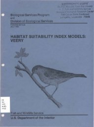
ACKNOWLEDGMENTSw. G. Layher (Kansas Fish and Game), L. L. Olmsted (Duke Power), andM. J. Van Den Avyle (Georgia Cooperative Fishery Research Unit) reviewed themanuscript and offered many constructive comments. C. Short provided editorialassistance and K. Twomey helped in the final preparation of the model.J. Shoemaker drew the cover illustration. Word processing was by C. Gulzowand D. Ibarra.

SPOTTED BASS (Micropterus punctulatus)HABITAT USE INFORMATIONGeneralThe spotted bass is native to the Southeastern United States, its northernrange extending into southern Illinois, Indiana, Ohio, and West Virginia(Robbins and MacCrimmon 1974). It has been introduced into streams in Arizona,New Mexico (Robbins and MacCrimmon 1974), California (Shapovalov et al. 1981),and in streams in Missouri and Kansas where it was not native (Cross 1967;Fajen 1975), as well as reservoirs in California (Shapovalov et al. 1981;Aasen and Henry 1981), Kansas, and throughout the Southeast (Robbins andMacCrimmon 1974). A detailed description of its distribution, including maps,is provided by Robbins and MacCrimmon (1975) and MacCrimmon and Robbins (1975).Three subspecies of spotted bass have been identified (Hubbs and Bailey1940): the Wichita spotted bass (~' £. wichitae) of West Cache Creek, Oklahoma(Ramsey 1975), the Alabama spotted bass- (~' £. henshalli) of the Mobile Baydrainage (Gilbert 1973), and the northern spotted bass (~. £. punctulatus)which occurs throughout the remainder of the range (Ramsey 1975). The wichitaesubspecies is presumed extinct (Cook 1979).Spotted bass is primarily a stream species and generally fares poorly inreservoirs except those having deep, clear, relatively infertile water andsteep, rocky shorelines (Jenkins 1975; Vogele 1975a; Webb and Reeves 1975).Spotted bass occupy a wide variety of stream types (Robbins and MacCrimmon1974; Vogele 1975a). They favor streams with moderate currents, rockysubstrates, and alternating pools and riffles (Cross 1967; Vogele 1975a; Smith1979). Spotted bass occupy stream habitats intermediate to those preferred bylargemouth bass (M. salmoides) and smallmbuth bass (M. dolomieui). The largemouthfrequents backwaters and other slack water areas, the smallmouth prefersfast-moving waters in or near riffles, and the spotted bass favors areas withslow to moderate currents (Ryan et al. 1970; Miller 1975; Vogele 1975a;Trautman 1981). In Mi ssouri, spotted bass are the most abundant of thecentrarchid basses in the main channels of larger rivers and in warm, gravelly,relatively turbid streams. In contrast, smallmouth bass predominate in cool,clear, high gradient streams and largemouth prefer clear, weedy, standingwaters (Fajen 1975; Pflieger 1975).1

Age, Growth, and FoodSpotted bass typically mature at age III-IV (Olmsted 1974; Voge1e 1975b).Olmsted (1974) found that in Lake Fort Smith, Arkansas, 34.2% of spotted basswere mature at age II, 85.5% at age III, and 100% at age IV.Spotted bass fry eat plankton and aquatic and terrestrial insects (Howland1931; Smith and Page 1969; Mullan and Applegate 1970; Ryan et a1. 1970).Larger spotted bass (> 75 mm TL) feed on insects, fish (centrarchids,c1upeids), and crayfish to varying degrees, depending on location, season, andavailability (Rosebery 1950; Smith and Page 1969; Mullan and Applegate 1970;Aggus 1972), but crayfi sh often predomi nate in the di et of spotted bass instreams (Howland 1931; Sca1et 1977), and in reservoirs (Aggus 1972; Bohn 1975;Lewis 1976). Numerous researchers have noted a close association betweenabundance of crayfish and abundance of spotted bass (Cross 1967; Voge1e 1975a).ReproductionTrautman (1981) and Lewisand E1 der (1953) noted that spotted bass inOhio and Illinois migrate upstream to spawn in tributaries of larger rivers astemperatures warm in the spri ng. Spotted bass spawn primari 1y in Apri 1 andMay (Voge 1e 1975a; Aasen and Henry 1981) as temperatures ri se above 14° to15° C (Ryan et al. 1970; Voge1e 1975a,b; Aasen and Henry 1981). Little nestbuilding or spawning occurs at temperatures < 15° C (Voge1e 1975b) or > 22° C(Aasen and Henry 1981).Eggs are laid in nests built and guarded by males (Voge1e 1975b). Instreams, nests are constructed in areas protected from current, but not inbackwaters (Pf1 ieger 1975). Coves and steep shore1 ines are used for nestingin reservoirs (Olmsted 1974; Voge1e 1975b; Aasen and Henry 1981). Spottedbass show a strong preference for nest building on rocky or other firmsubstrate near cover of logs, brush, or clumps of submerged vegetation (Howland1932; Olmsted 1974; Voge1e 1975b; Voge1e and Rainwater 1975; Aasen and Henry1981). Nest depths generally are greater than other centrarchid basses (Voge1e1975a; Aasen and Henry 1981). The mean depth of nests was reported as 2.3 to3.7 m in Bull Shoals Reservoir, Arkansas (Voge1e 1975b), and 2.7 m in LakePerris, California (Aasen and Henry 1981).Embryos hatch within 5 days at temperatures near 15° C (Voge1e 1975b).Fry form schools near shoreline cover and are guarded by males until theydisperse (Voge1e 1975b).Specific Habitat RequirementsSubstrate type and current appear to be major physical determinants ofhabi tat sui tabi 1ity for spotted bass in streams. Streams where spotted bassare most abundant are characterized by rocky substrates; large, deep pools;and well-defined riffles (Howland 1931; Ryan et a1. 1970; Robbins andMacCrimmon 1974; Fajen 1975). Large, deep pools provide resting cover andspawning habitat; rocky substrates provide suitable habitat for production of2

aquatic insects (Hynes 1970) and crayfish (Loring and Hill 1976) used as foodby spotted bass. Fajen (1975) reported that stocking success of spotted bassin Missouri streams devoid of centrarchid basses was highest in those streamswith the above features and very low in streams with substrates comprised ofshifting sand or silt. A decline in spotted bass populations after channelizationof streams in Louisiana was noted by Robbins and MacCrimmon (1974).Turbidity appears to be a less significant factor in the suitabil ity of astream as spotted bass habitat. The spotted bass is more tolerant of turbiditythan smallmouth bass (Fajen 1975; Pflieger 1975) and is found in streams ofvaryi ng turbidity throughout its range. Layher (1983), however, found thatstanding crops of spotted bass in Kansas were largest in stream sites with lowto moderate levels of turbidity (~ 60 JTU's).Substrate type, turbidity, fertil ity, and depth appear to be the majorfactors affecting habitat suitability of reservoirs for spotted bass (Olmsted1974; Jenkins 1975; Vogele 1975a). Jenkins (1975) reported that standingcrops of spotted bass in reservoirs were positively correlated with mean depthand negatively correlated with total dissolved solids (lOS). Steep, rockyshorelines are a characteristic feature of reservoirs where spotted bass areabundant (Roseberry 1950; Olmsted 1974; Vogele 1975a; Webb and Reeves 1975).Spotted bass are restricted to fresh water; Bailey et al. (1954) reportedthat they are absent from waters along the Gulf Coast with salinities exceeding1 ppt. Based on the pH requirements and tolerances of largemouth and smallmouthbass (Bulkley 1975), a pH range of 6.0 to 9.5 is considered to be suitablefor survival of all life stages of spotted bass. Layher (1983) foundthat adult spotted bass standing crops were highest in those Kansas streamshaving a pH value between 8.5 and 9.0.Adult. Adult spotted bass in rivers prefer deep areas with slight tomoderate current (Ryan 1970; Vogele 1975a; Trautman 1981). They tend to avoidareas of soft mud substrate, dense emergent vegetation, or fast current(Howland 1931; Fajen 1975; Vogele 1975a). In reservoirs, adult spotted bassare generally found near deep, rocky, littoral areas or reefs (Olmsted 1974;Robbins and MacCrimmon 1974; Vogele 1975b), as well as deep, open water abovethe thermocline (Dendy 1945; Stroud 1948). As in streams, they tend to avoidreservoir areas with soft mud substrate and dense vegetation (Olmsted 1974).In Lewis Smith Reservoir, Alabama, spotted bass showed a strong attraction toman-made structures added to increase cover in open water (Smith et al. 1980).Adult spotted bass grow best at temperatures near 24° C (Mohl er 1966).Dendy (1945) and Stroud (1948) reported that spotted bass in Norris Reservoir,Tennessee, were most abundant in epilimnetic areas with temperatures of 23.5to 24.4° C. The upper lethal temperature range for spotted bass is undetermined,but is probably near 34° C (Robbins and MacCrimmon 1974). Spotted bassgrowth is greatly reduced at temperatures ~ 15.5° C and ceases at temperatures~ 10° C (Mohler 1966). Adult spotted bass can survive dissolved oxygen (D.O.)levels near 1 mg/l for short periods, but D.O. levels ~ 6 mg/l are optimum forlong term survival and growth (Mohler 1966).3

Embryo. Because nests in reservoirs are often built in relatively deepwater (Vogele 1975b; Aasen and Henry 1981), spring reservoir drawdown may be1ess detrimental to reproduction of spotted bass than it is to other centrarchidbasses which construct much shallower nests (Aasen and Henry 1981).The strong preference shown by spotted bass for nest building on firmsubstrates near cover (Olmsted 1974; Vogele 1975b; Aasen and Henry 1981)suggests that substrate type and cover are important features in determiningsuitability of habitat for reproduction of spotted bass.The temperature and dissolved oxygen (D.O.) requirements for embryos areunknown. Presumably, temperatures of 18 to 21° C are optimum for growth andsurvival of embryos, because these temperatures occur during peak spawningactivity (Ryan et al. 1970; Vogele 1975a,b; Aasen and Henry 1981). D.O.requirements are likely to be similar to those of small mouth bass (Siefertet al. 1974); thus, D.O. levels of ~ 6 mg/l may be considered optimum forsurvival and growth, and D.O. levels s 1.5 mg/l would be lethal.Fry. Little is known about the distribution or habitat requirements ofspottea-bass fry. In reservoirs, fry seek shoreline cover after leaving nests(Vogele 1975a). The amount of cover available to spotted bass for spawningand as fry habitat may directly effect reproductive success and year-classstrength in reservoirs (Vogele and Rainwater 1975). Oxygen and temperaturerequirements of spotted bass fry are unknown but are assumed to be similar tothose of adults.Juveniles. Little is known about specific habitat requirements forjuvenile spotted bass as their requirements are rarely differentiated fromthose of adults in the literature. In Center Hill Reservoir, Tennessee,Jahnke (1979) did not observe substrate preferences for either age 0 or age Ijuvenile bass. Age 0 fish also showed no location preference but age I basswere most abundant in inner cove habitats. Thus, juvenile spotted bass do notappear to show the strong preference for rocky substrates as reported foradults (Olmsted 1974; Vogele 1975a; Roussel 1979).HABITAT SUITABILITY INDEX (HSI) MODELSModel ApplicabilityGeographic area. The models were designed to evaluate the suitability ofwater bodies within the native and introduced range of spotted bass. Thestandard of comparison for each suitability index is the optimum value of thevariable that occurs anywhere within this geographic range. Users of thesemodel s should use the Habitat Use Information section of this model, as wellas local information, to adapt this model to local conditions.Season. The models are designed to rate a riverine or lacustrine habitaton its ability to support a self-sustaining population of spotted bass throughoutthe yea r.4

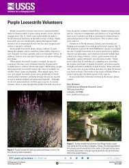
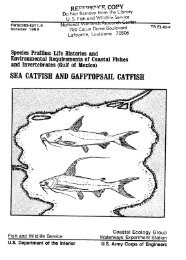
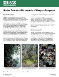
Cover types. Models are applicable to riverine and lacustrine habitats,as defined by Cowardin et al. (1979).Verification level. These model s have not been tested against habitatsof known qual ity. Layher and Maughan (1982) tested an earl ier version of ari veri ne mode1 for spotted bass havi ng gradi ent, substrate, temperature, andaverage velocity as model variables. HSI (computed as the geometric mean ofsuitability index values for each variable) was not significantly (p > 0.10)correlated with standing crop of spotted bass in 46 stream sites in Kansas,but a trend towards increasing standing crops of spotted bass with higher HSIvalues was evident. Suitability index (SI) graphs for substrate and temperaturewere found to closely approximate SI curves derived by transformingspotted bass standing crop values to SIl s as described in USFWS (1981).Failure of the tested model was attributed to the use of the geometric mean tocalculate HSIls and to the absence of limiting variables from the model.Layher (1983) found that mean width, minimum width, percent riffle, pH,turbidity, temperature, and nitrates accounted for most of the variation instanding crop of spotted bass in Kansas streams. This information was used indeveloping SI graphs for the riverine HSI model presented here. Mean width,minimum width, and nitrates were excluded as model variables since they wereconsidered either correlates of other model variables or would not be usefulin evaluating habitats under future conditions.Model Description -RiverineOverview. The HSI model is an attempt to condense information on habitatrequirements of spotted bass into a set of habitat evaluation criteria. Themodel includes those variables with a known impact on the growth, survival,distribution, abundance, standing crop, and/or preferences of spotted bass,and thus could be expected to have an impact on the carrying capacity of ahabitat. The model is structured to produce a relative index of the abilityof a present or future habitat to meet the food and cover, water quality, andreproductive requirements of spotted bass. The hypothetical relationshipbetween habitat variables, model components, and HSI is illustrated inFi gure 1.The following sections document why a particular set of habitat variableswere chosen for each model component. The definition and justification of thesuitability levels of each model variable are described in the SuitabilityIndex Graphs section.5

TurbidityV spH V 6Water Quality HSITemperature - summer V 7D.O. V 9Substrate type--------V 3Percent cover-------- V,.Temperature - spawning ---- Vaf-------- Reproduct ionD.O. - spawning ------- V 1 0Figure 1. Diagram illustrating habitat variables in the riverine HS1model and the aggregation of the corresponding suitability indices(SI's) into an HS1. HS1 = the lowest of the 9 suitability indexratings.6

Food/cover component. The 1i terature documents a wi de va ri ety of foodtypes eaten by spotted bass, but crayfi sh are often reported as a primarycomponent of the diet. Percent rocky substrate (V 3 ) was included in thiscomponent because crayfi sh are most abundant in rocky substrates whi ch theyrequire for shelter (Loring and Hill 1976). V 3 should also provide an 'indexof aquatic insect availability, a seasonally abundant food item for spottedbass in at least some streams (e.g., Smith and Page 1969), because aquaticinsect production is highest on rocky substrates (Hynes 1970). V 3 also wasincluded in this component because numerous sources document that spotted bassare most abundant in gravel-bottomed streams. Layher and Maughan (1982)provided data that standing crop Gf spotted bass is proportional to the amountof rocky substrate present.Percent riffles (V 1 ) was included in this component because (1) spottedbass streams commonly have alternating pool s and well-defined riffles, and(2) Layher (1983) found that standing crop of spotted bass in Kansas streamsvaried with percentage of riffles present. Similarly, pool depth (V z ) wasincluded because spotted bass are most abundant in streams with large, deeppools (Howland 1931; Ryan et al. 1970; Fajen 1975).Structural cover (V 4 ) of logs, boulders, and brush are common in streamswhere spotted bass are found and thus was included in this component. Also,it seems that increased cover provides more suitable habitat for forage fisheseaten by spotted bass in streams (i .e., cyprinids and centrarchids).Water quality component. Turbidity (V s ) was included as a variable inthis component because spotted bass are most abundant in clear to moderatelyturbid conditions (e.g., Pflieger 1975) and are intolerant of conditionsassociated with high turbidity (e.g., high siltation) (Smith 1979).This component includes pH (V G ) because pH is a known limiting factor offish populations. In addition, Layher (1983) found evidence that standingcrop of spotted bass in streams varies with pH level.Spotted bass occur over a wide latitudinal range, but seem to prefertemperatures (V 7 ) somewhat intermediate to those preferred by smallmouth bassand largemouth bass. Standing crop of spotted bass in Kansas streams washighest at summer temperatures of 24 to 27° C.Relatively little is known about D.O. (V 9 ) requirements of spotted bass.As with the other centrarchid basses, they are probably tolerant of short termdecreases in D.O. to 2 mg/l, but long term D.O. levels below 3 mg/l are probablylimiting. Layher (1983) did not find spotted bass in Kansas streams withD.O. levels below 4 mg/l.7

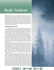
Reproduct i on component. Spawni ng requi rements of spotted bass appearrelatively flexible, although they do exhibit preferences for building nestson firm substrates near cover (Vogele 1975b). V 3 and V 4 were included in thiscomponent as measures of these preferences. Measurements of temperature (Va)and D.O. (V i O) are included in this component in as much as nesting successwill depend on the suitability of these variables' values during the springspawning period.HSI determination. It was assumed that the most limiting factor (i .e.,lowest SI score) defines carrying capacity for spotted bass in rivers; thus,the HSI equals the rn i nimum value of any of the suitability indices Vi to ViO.ModelDescription - LacustrineOverview. Spotted bass usually are a minor component of centrarchid bassstanding crop in reservoirs (largemouth bass are more prevalent), except inreservoirs characterized by deep, clear, relatively infertile water and steep,rocky shorelines. Model variables were chosen that provide measures of thesereservoir habitat characteristics for spotted bass. The relationship betweenlacustrine habitat variables, model components, and HSI is illustrated inFigure 2. The "other" component comprises a variable that affects habitatsUitability for spotted bass, but which does not fit easily into food/cover,water quality, or reproduction components of the model.Food/cover component. The literature characterizes spotted bass as mostabundant in reservoirs with rocky substrates and as avoiding reservoir sectionswith mud substrate and dense emergent vegetation; thus, percent rocky substrate(V 3 ) was included in this component. Aggus (1972) found that crayfish, aprimary food item of spotted bass in reservoirs, were closely tied to rockysubstrates in Bull Shoals Reservoir, Arkansas. Percent cover (V 4 ) was alsoincluded in this component since spotted bass are attracted to rocky outcroppingsand man-made midwater structures. Again, it seems that more availablecover indicates a more suitable habitat for forage fishes utilized by spottedbass.Water quality component. Turbidity (V s) was included in this componentbecause reservoirs with high populations of spotted bass are commonly characterizedin the literature as having clear water. For the model variables ofpH (V 6 ), temperature (V 7 ), and D.O. (V g ), see the explanations presented inthe water quality component of the riverine HSI model.Reproduct i on component. Spotted bass in reservoi rs prefer rockysubstrates (V 3 ) near log or brush cover (V 4 ) as nest sites. Due to thispreference and deeper nest depths, spotted bass appear to do better than othercentrarchid basses in reservoirs that have fluctuating water levels in springand/or rocky, relatively barren substrates predominating along the shorelineas in Lake Perris, California (Aasen and Henry 1981) and Lewis Smith Reservoir,Alabama (Webb and Reeves 1975; Smith et al. 1980).8

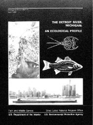
Habitat variablesSuitabil ityindicesLHe regui sitesSubstrate type --------V3~,------r-r-Food/CoverPercent cover-------- V 4Trophic status-------- V ll- - - - - - - Other ------'Figure 2. Diagram illustrating habitat variables in the lacustrineHSI model and the aggregation of the corresponding suitabilityindices (Sl ls) into an HS1. HSI = the lowest of the 10 sUitabilityindex ratings.9

For explanations on why temperature (Va) and D.O. (V 1 0 ) were included inthis component, see the water quality component of the riverine HSI model.Other component. Trophi c status (V 11) was i ncl uded as a measure ofhabitat suitabi 1ity for spotted bass because ferti 1ity and mean depth havebeen identified by regression analyses and observation as variables highlylikely to affect the population abundance of spotted bass in reservoirs (seeHabitat Use Information section). A general trophic class rating system isthought to be a more representative and useful system of rating than specificSI graphs for TDS and mean depth because available information is only of ageneral nature. Deep, relatively oligotrophic reservoirs define the optimumlacustrine habitat for spotted bass. Examples of reservoirs with thesecharacteristics, and that have high standing crops of spotted bass, are:MeanReservoir/location Fertility depthCenter Hill, Tennessee TDS = 115 mg/l 24 m(MEl = 4.8)Bull Shoals, Arkansas* TDS = 150 mg/l 22 m(MEl = 6.8)*Secchi depth = 8.4 mAllatoona, Georgia TDS = 40 mg/l 10.3 m(MEl = 3.9)Lewis Smith, Alabama low 30 mClaytor, Virginia low highReferencesHargis 1965; Leidy andJenkins 1977Leidy and Jenkins 1977;Vogele 1975aKirkland 1965; Leidyand Jenkins 1977Webb and Reeves 1975Roseberry 1950In contrast, spotted bass populations do poorly in shallow, eutrophic impoundmentseven if they were common in the stream prior to impoundment (Patriarche1953; Vogele 1975a).HSI determination. The most limiting factor (i .e., lowest SI score) wasassumed to define carrying capacity for spotted bass in reservoirs; thus, HSIequals the minimum value for suitability indices V 3 through V 1 1 •Suitability Index (SI) Graphs for ModelVariablesTable 1 lists the rationale and assumptions used in constructing each SIgraph. Graphs were constructed by converting ava il abl e i nformat i on on thehabitat requi rements of spotted bass into an index of suitabil ity from 0.0(unsuitable) to 1.0 (optimum). Descriptors for each habitat variable werechosen to emphasize limiting conditions for each variable. This choicereflects our assumption that extreme, rather than average, values of a variablemost often limit the carrying capacity of a habitat. (R) refers to Riverineand (L) to Lacustrine model variables.10

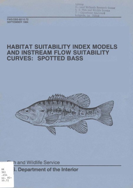
1.0Habitat Variable x 0.8R Vi Percent riffles duringlow summer flow period.Q)"'0c .......>,oj.J0.6.,.....,....r-(Riffle = areas where 0.4.0substrate projectsIt!oj.Jabove water surface.,....:::lor where flow is0.2Vlturbulent.)0.00 20 40 60 80 100%R V 2 Average pool depth 1.0during low summerflow period.x0.8Q)"'0(Suggested measure-c....... 0.6ment = average of>,pool depths at 1 moj.Jintervals across 0.4transects.).,.....0It!oj.J.,....:::lVl0.20.00 2 3 4 5mR,L V 3 Percent of substrate 1.0in streams (R) orreservoirs (L) com- x 0.8Q)prised of gravel,cobble, boulders,or bedrock. >,oj.J"'0c ....... 0.6.,....r-.,.....0It!oj.J'r-:::lVl0.40.20.00 10 20 30 40 >50%11

R,L V 4 Percent cover 1.0(boulders, brush,log piles, or other~ 0.8structure) in pools"'0l::(R) or above thermo-......cline in reservoirs >. 0.6~(L) ..r-:;::: 0.4..a ro~oS 0.2(/)0.00 10 20 30 40 >50%R,L V s Average turbidity 1.0during summer.~ 0.8"'0l::......>. 0.6~.r-:;::: 0.4..a ro~.; 0.2(/)0.00 30 60 90 120JTUR,L V 6 Annual maximum or 1.0minimum pH. (Usemeasurement withlowest 51 value.)x0.8(l)"'0l::...... 0.6c-,~;:: 0.4.r-..a ro~ 0.2::::s(/)0.04 6 8 10 12ph12

R,L V 7 Average maximum daily 1.0temperature duringwarmest summer month.(For 1acustri ne~ 0.8"'Capplications (L),c ......the 51 value is c-, 0.6the most suitable ..... +->temperature above:-;=: 0.4the thermocline..t:l(lJduring the month.+->.; 0.2U')0.010 15 20 25 30 35°CR,L Va Minimum temperature 1.0during spawning(Apri 1 to May).For example, ifx 0.8Q}temperature declines"'Ccto 15° C when bass ...... 0.6are spawning, then c-,+->51 = 0.2. ;:: 0.4..t:l(lJ~ 0.2~U')0.010 15 20 25 30°CR,L Vg Minimum dissolved 1.0oxygen levels duringsummer, fa 11 , andx 0.8winter in pools (R) Q}"'Cor at locationcselected for most ...... 0.6>,suitable temperature+->for variable V 7 (L). :-;::: 0.4..t:l(lJ+->.; 0.2U')0.00 2 4 6 >8mg/l13

R,L V lO Minimum dissolved 1.0oxygen 1eve1 determinedat same timexand location as0.8OJ"0for Va.t::......>, 0.6-+J-r-:'r- 0,4..0ttl-iJ'r-:;, 0.2(/)L V ll Trophic status/productivity of lakeor lake section.0.0LOx 0.8OJ"0A B C t::(Oligo- (Meso-......>, 0.6Parameter 1 trophic) trophic) (Eutrophic) -iJ.r-'r-Productivity low medium high 0.4..0ttl-iJ'r-Sedimentation:;, 0.2(/)rate low medium high0 2 4 6 >8Nutrient000levels A B C(mg/m 3-p) < 9 9-18 > 18MorphoedaphicIndex (MEI)2 < 6.0 6-7.2 > 7.2Transparency(Secchidepth) > 6 m 1-6 m < 1 mmg/lITable adapted from Leach et a1, (1977) .2MEI = TOS(mg/l)/mean depth (m),14

Table 1. Sources of information and assumptions used in constructionof the suitability index graphs. "Excellent" habitat for spotted bassrefers to an SI of 0.8 to 1.0, "good" an SI of 0.5 to 0.7, "fair" 0.2to 0.4, and "poor" habitat 0.0 to 0.1.VariableAssumptions and sourcesSpotted bass are most abundant in streams with well-definedriffles and deep pools (Howland 1931; Lewis and Elder 1953; Ryanet al. 1970; Fajen 1975; Trautman 1981), therefore, a mixture ofriffles and pools is considered excellent. Zero percent rifflesis considered poor habitat because spotted bass are rare inbackwaters and other areas lacking at least some current (Fajen1975; Vogele 1975a; Ryan et al. 1970). High percent riffles isalso poor because: (1) spotted bass in streams occupy large,deep pools (Howland 1931; Fajen 1975); (2) channelizationadversely affects spotted bass populations (Robbins and MacCrimmon1974); and (3) stocking success of spotted bass was very poor inrivers with extensive channelization (Fajen 1975). The generalshape of the graph for Vi was based on the following standingcrop data from Kansas streams (Layher 1983):Fraction ofPercent No. of Mean maximum mean standingriffles stream sites standing crop crop = SI< 15 302 0.82 0.2515-30 62 2.09 0.6230-45 26 3.35 1. 0045-60 5 0.00 0.0060-7575-90 3 0.00 0.00> 90 1 0.00 0.00Shallow pools are deemed poor because stocking success (Fajen1975) and abundance of spotted bass (Howland 1931; Trautman 1981)is low in streams where shallow pools predominate. Average pooldepths ~ 1 m are rated good to excellent because spotted bass aremost abundant in large, moderately deep pools (Howland 1931; Ryanet al. 1970; Robbins and MacCrimmon 1974; Fajen 1975; Trautman1981) and standing crop of spotted bass was highest in Kansasstreams having mean depths 1.2 to 1.8 m (Layher 1983). Spottedbass prefer areas with some current, which is most characteristicof small- to moderate-sized streams « 30 m wide) (Ryan et al.1970; Robbins and MacCrimmon 1974; Vogele 1975a; Layher 1983),thus, the suitability of depths ~ 5 m was determined to be onlyfair.15

Table 1.(continued).VariableAssumptions and sourcesIt is assumed that habitat suitability is proportional to theamount of rocky substrates present in streams and reservoirsbecause: (1) spotted bass are most abundant in streams (Howland1931; Lewis and Elder 1953; Cross 1967; Fajen 1975; Layher andMaughan 1982), reservoirs (Roseberry 1950; Aasen and Henry 1981),and reservoir sections (Olmsted 1974; Roussel 1979) with rockysubstrates; (2) spotted bass prefer rocky substrates as spawningsites (Olmsted 1974; Vogele 1975b; Aasen and Henry 1981);(3) crayfish are a primary component of the diet of spotted bassand crayfish are most abundant in rocky substrates that providethem shelter (Aggus 1972; Emery 1975; Loring and Hill 1976); and(4) spotted bass, especially juveniles (e.g., Smith and Page1969), eat aquatic insects and production of aquatic insects ishighest on gravel-cobble substrates (Hynes 1970). Spotted bassare absent from areas of dense emergent vegetation and mud bottom(Olmsted 1974), and stocking was unsuccessful in Missouri streamswith shifting sand substrate (Fajen 1975), therefore thesesubstrate types are deemed poor.The strong preference of spotted bass for building their nestsnear brush or other forms of cover (Vogele 1975b; Vogele andRainwater 1975; Aasen and Henry 1981), the use of cover by fryafter leaving their nests (Vogele 1975b), the attraction ofspotted bass to man-made midwater structures (Smith et al. 1980)and rocky outcroppings in reservoirs (Robbins and MacCrimmon1974), and the common listing of abundant cover as a habitatcharacteristic of spotted bass streams (e.g., Viosca 1932; Ryanet al. 1970), suggests that some cover is necessary for optimumconditions. Zero percent cover is assigned an SI of 0.2 becausea stream or reservoir may still be able to support spotted bass,although at a much reduced level. The selection of ~ 25% cover asoptimum is our best estimation based on available information.Although spotted bass are found over a wide range of turbidities(Robbins and MacCrimmon 1974; Vogele 1975a), low turbidities areconsidered excellent because spotted bass are most abundant inclear streams and reservoirs (e.g., Lewis and Elder 1953; Cross1967; Olmsted 1974; Vogele 1975a; Webb and Reeves 1975). The SIgraph was constructed primarily on the basis of the followingstanding crop data from Kansas streams (Layher 1983):16

Table 1.(continued).VariableAssumptions and sourcesMeanFraction ofTurbi dity No. of standing crop maximum mean standing(JTU's) stream sites (Kg/ha) crop = 510-30 161 1.77 1. 0030-60 49 1. 54 0.8760-90 18 0.61 0.3590-120 10 0.01 0.01120-570 15 0.00 0.00V 6 Levels of pH in the range of 6.0 to 9.5 are generally consideredsuitable for centrarchid basses (Bulkley 1975). Thegeneral shape of the graph was based on the following standingcrop data from Kansas streams (Layher 1983):MeanFraction ofNo. of standing crop maximum mean standingpH stream sites ( Kg/ha) crop = 51< 6.5 3 0.00 0.00~ 6.5-6.99 10 0.88 0.38~ 7.0-7.49 39 0.21 0.09~ 7.5-7.99 114 0.61 0.27~ 8.0-8.49 149 1. 01 0.44~ 8.5-8.99 72 2.30 1.00~ 9.0-9.49 14 0.00 0.00Unsuitable pH levels were determined by the levels that werelethal to largemouth bass in laboratory experiments [< 4.2 and> 10.3 (Calabrese 1969)].17

Table 1. (continued).VariableAssumptions and sourcesTemperatures associated with highest growth in laboratory experiments[24° C (Mohler 1966)J, highest abundance in reservoirs[23.5 to 24.4° C (Dendy 1945; Stroud 1948)J, and highest standingcrops in Kansas streams (see below) are rated excellent. Temperaturesthat (1) are assumed lethal to spotted bass [~ 34° C(Robbins and MacCrimmon 1974)J, (2) are avoided [> 34° C (Cherryet al. 1975)J, or (3) corresponded to an absence of spotted bassin Kansas streams (~ 32° C), are deemed poor as are temperaturesassociated with little or no growth [< 15° C (Mohler 1966)J andvery low standing crops [< 12 to 16° C (Layher 1983)J. The shapeof the graph between optimum and no sUitability was based on thefollowing standing crop data from Kansas streams (Layher 1983):MeanFraction ofTemperature No. of standing crop maximum mean standinginterval stream sites (Kg/ha) crop = SI~ 12-15 27 0.02 0.01~ 16-19 45 0.45 0.20~ 20-23 98 1.10 0.50~ 24-27 129 2.15 1.00> 28-31 41 0.89 0.40~ 32-35 3 0.00 0.00~ 36-39 1 0.00 0.00Temperatures coinciding with highest incidence of spawning [17to 21° C (Ryan et al. 1970; Olmsted 1974; Vogele 1975a,b; Aasenand Henry 1981)J are excellent. Temperatures above [> 23° C(Vogele 1975a,b; Aasen and Henry 1981)J or below [< 15° C (Olmsted1974; Vogele 1975a,b; Aasen and Henry 1981)J the range wherenesting has been observed are poor.V 9 D.O. levels coinciding with highest growth and survival of spottedbass [~ 6 mg/l (Mohler 1966)J are excellent. Levels that arelethal to spotted bass [< 1 mg/l (Mohler 1966)J or that elicitavoidance in largemouth bass [< 1.5 mg/l (Whitmore et al. 1960)Jare poor. D.O. levels < 5 mg/l are less than optimum becauseswimming speed (Dahlberg et al. 1968) and production (Warrenet al. 1973) of largemouth bass decreases below this level.18

Table 1.(concluded).VariableAssumptions and sourcesNo information was available on D.O. requirements of spotted bassembryos. D.O. levels lethal to smallmouth bass embryos in thelaboratory [< 2.5 mg/l (Siefert et al. 1974)J are therefore usedhere, and are considered to be poor. Levels coinciding with areduction in survival of smallmouth bass embryos are rated fair[< 4 mg/l (Siefert et al. 1974)J. Levels ~ 6 mg/l are assumed tobe excellent for spawning and embryo survival of spotted bass.Spotted bass are most abundant in deep, relatively infertilereservoirs (Roseberry 1950; Jenkins 1975; Webb and Reeves 1975;Vogele 1975a), therefore, oligotrophic-mesotrophic conditions areconsidered to be excellent. Eutrophic conditions are consideredto have fair-poor suitability because largemouth bass are moreabundant than spotted bass under these conditions (Patriarche1953; Olmsted 1974). Because growth of spotted bass in highlyoligotrophic Lake Fort Smith, Arkansas (total alkalinity = 10 to30 ppm) was very low (Olmsted 1974), we assumed that reservoirswith very low fertility would be less suitable.Interpreting ModelOutputsThe riverine and lacustrine models described above are generalizeddescriptors of habitat requirements of spotted bass and thus the model outputshould not be expected to discriminate among different habitats with a highdegree of resolution (Terrell et al. 1982).A spotted bass HSI determined by application of the models may not reflectthe population level of spotted bass in the study area since other variablesmay have a more significant influence in determining spotted bass abundance.A positive relationship between HSI's generated by these models and themeasureable indices of population abundance (e.g., standing crop) is assumed,but this hypothesized relationship has not been tested other than by inferencesdrawn from the literature during the model-building process. The properinterpretation of the HSI is one of comparison. If two areas have differentHSI's, the area with the higher HSI should have the potential to support morespotted bass than the one with the lower HSI. Outputs of these models shouldbe interpreted as indicators (or predictors) of excellent (0.8 to 1.0), good(0.5 to 0.7), fair (0.2 to 0.4), or poor (0.0 to 0.1) habitat for spottedbass.The models should be useful as a basic framework for formulating revisedmode 1s that incorporate site-specifi c or project-specifi c factors affect i ng19

habitat suitability for spotted bass (see Terrell et al. 1982). The individualsuitability indices may also be useful for identifying habitat variables thatmay be limiting, without aggregating the SIl s into an HSI. Results of testingan earlier version of a riverine HSI model for spotted bass (Layher 1983)suggest an important point. That is, if a more precise index of populationabundance is required, use of the HSI models derived from suitability indicesaggregated by nonstatistical methods may not be appropriate or should bepreceded by evaluating the model in the field. Testing the model will betterdefine which variables are important descriptors of habitat quality in theproposed area of model application or under the post-project conditions.ADDITIONAL HABITAT MODELSDescriptive ModelsThe following models are simplified descriptions of optimum habitat forspotted bass as detailed in the Habitat Use Information section of thissummary. These models should be useful for "reconnaissance-grade" applicationswhere the relative quality of habitats for spotted bass must be judged usingminimal data.Riverine model. Optimum riverine spotted bass habitat (assuming waterquality is not limiting) is characterized by:1. Average summer temperatures in the range of 20 to 24° C;2. Rocky substrates;3. An approximate 3:2, pool :riffle ratio; and4. Cover present in pools.HSI = number of attributes present4Lacustrine model. Optimum lacustrine spotted bass habitat (assumingwater quality is not limiting) is characterized by:1. Summer water temperatures in the range of 20 to 24° C, .with adequateD.O. levels are available;2. Rocky substrates;3. Low turbidity (> 5 m Secchi depth);20

4. Deep (mean depth> 15 m); and5. Low fertility (TDS< 125 but> 50 mg/l).HSI = number of attributes present5Regression ModelsLayher (1983) developed regression equations to predict standing crop ofspotted bass in streams in Kansas and Oklahoma. In Kansas, habitat variablesof turbidity, mean depth, minimum width, mean width, pH, percent riffles, andtemperature accounted for the significant variation in standing crop. Meanwidth, pH, turbidity, temperature, nitrates, mean depth, and minimum widthexplained the variation in standing crop in Oklahoma streams. Layher (1983)reports the methods of analysis and provides guidance on potential use of themodels to predict standing crop. The regression equations utilize SI's derivedfrom SI graphs as the independent variables. Graphs and equations arepresented in Layher (1983). Further information on their use may be obtainedfrom: William G. Layher, Environmental Services Section, Kansas Fish andGame, Pratt, Kansas 67124.Aggus and Morais (1979) developed regression equations to predict standingcrop of spotted bass in reservoirs from easily obtainable preconstructiondata. These authors discuss procedures for converting measured or predictedstanding crop values for spotted bass to HSI's.Discriminant Analysis ModelsLayher (1983) used discriminant analysis to determine the relationshipsbetween habitat variables and presence or absence of spotted bass in streamsin Kansas and Oklahoma. The discriminant analysis models showed high reliabilityfor predicting presence or absence of spotted bass within each data set.When the Kansas model was applied to Oklahoma streams, however, many misclassificationsresulted, suggesting that the models are reliable only overlimited, homogeneous geographical areas. Further information on use of thesediscriminant models can be obtained by contacting William G. Layher at theaddress listed in the Regression Models section.INSTREAM FLOW INCREMENTAL METHODOLOGY (IFIM)The U.S. Fish and Wildlife Service's Instream Flow Incremental Methodology(IFIM), as outlined by Bovee (1982), is a set of ideas used to assess instreamflow problems. The Physical Habitat Simulation System (PHABSIM), described byMilhous et al. (1984), is one component of IFIM that can be used by investigatorsinterested in determining the amount of available instream habitat21

for a fish species as a function of streamflow. The output generated byPHABSIM can be used for several IFIM habitat display and interpretationtechniques, including:1. Optimization. Determination of monthly flows that minimize habitatreductions for species and life stages of interest;2. Habitat Time Series. Determination of the impact of a project onhabitat by imposing project operation curves over historical flowrecords and integrating the difference between the curves; and3. Effective Habitat Time Series. Calculation of the habitat requirementsof each life stage of a fish species at a given time by usinghabitat ratios (relative spatial requirements of various lifestages).Suitability Index Graphs as Usedin IFIMPHABSIM utilizes Suitability Index graphs (SI curves) that describe theinstream suitability of the habitat variables most closely related to streamhydraulics and channel structure (velocity, depth, substrate, temperature, andcover) for each major life stage of a given fish species (spawning, eggincubation, fry, juvenile, and adult). The specific curves required for aPHABSIM analysis represent the hydraulic-related parameters for which a speciesor life stage demonstrates a strong preference (i.e., a species that onlyshows preferences for velocity and temperature will have very broad curves fordepth, substrate, and cover).Four categories of SI curves are described below. All species curves forHEP and IFIM are referred to collectively as suitability index (SI) curves orgraphs. The designation of a curve as belonging to a particular category doesnot imply that there are differences in the quality or accuracy of curvesamong the four categories.Category one curves are the most common type presently available for usewith HEP or IFIM. Usually category one curves have as their basis one or more1iterature sources. Some SI curves may be derived from general statementsmade in the literature about fishes (i.e., rainbow trout spawn in gravel; fryprefer shallow water.). Some category one curves may come from literaturesources which include variable amounts of field data (i .e., from a sample sizeof 300, fry were observed in velocities ranging 0.0 to 3.0 ft/sec, and 80%were found in velocities less than 1.0 ft/sec). Other category one curves maybe based entirely on professional opinion, by using the Delphi technique oreducated guesswork (i .e., an expert believes that velocities ranging 1.0 to8.0 ft/sec are necessary for successful spawning of striped bass). Mostcategory one curves are the result of a combination of sources; the finalcurve may include information from the literature, combined with field data,and smoothed or modified using professional judgement. Category one curvesusually are intended to reflect general habitat suitability throughout theentire geographic range of the species and throughout the year, unless they22

are identified as being applicable only to a given area or season. In thelatter case, curves developed for a specific area or stream may not accuratelyreflect habitat utilization in other areas. Curves meant to describe thegenera1 habi tat sui tabi 1i ty of a vari ab 1e throughout the entire range of aspecies may not be as sensitive to small changes of the variable within aspecific stream (i .e., rainbow trout will generally utilize silt, sand, gravel,and cobble for spawning substrate, but utilize only cobble in Willow Creek,Colorado).Category two curves are derived from frequency analyses of field data,and are basically curves fit to a frequency histogram. Each curve describesthe observed utilization of a habitat variable by a life stage. Category twocurves unaltered by professional judgement or other sources of information arereferred to as utilization curves. When modified by judgement they thenbecome category one curves. Utilization curves from one set of data are notapplicable for all streams and situations (i .e., a depth utilization curvefrom a shallow stream cannot be used for the Mi ssouri River). Category twocurves, therefore, are usually biased because of limited habitat availability.An ideal study stream would have all substrate and cover types present inequal amounts; all depth, velocity, and percent cover intervals available inequal proportions; and all combinations of all variables in equal proportions.Util ization curves from such a perfectly designed study theoretically shouldbe transferable to any stream within the geographical range of the species.Curves from streams with high habitat diversity, then, are generally moretransferable than curves from streams with low habitat diversity. Users of acategory two curve should first review the stream description to see if conditionsare similar to those present in the stream segment to be investigated.Some variables to consider might include stream width, depth, discharge,gradient, elevation, latitude and longitude, temperature, water quality,substrate and cover diversity, fish species associations, and data collectiondescriptors (time of day, season of year, sample size, sampling methods). Ifone or more deviate significantly from those of the proposed study site, thencurve transference is not advised, and the investigator should develop his owncurves.Category three curves are derived from utilization curves which have beencorrected for envi ronmenta1 bi as and therefore represent preference of thespecies. To generate a preference curve, one must simultaneously collecthabitat utilization data and habitat availability data from the same area.Habitat availability should reflect the relative amount of different habitattypes in the same proportions as they exist throughout in the s t ream-studyarea. A curve is then developed for the habitat frequency distribution in thesame way as for fish utilization observations, and the equation coefficientsof the availability curve are subtracted from the equation coefficients of thethe utilization curve, resulting in preference curve coefficients. Theoretically,category three curves should be unconditionally transferable to anystream, although this has not been validated. At present, very few categorythree curves exist because most habitat utilization data sets are withoutconcomitant habitat availability data sets. In the future, the need to collecthabitat availability data will be impressed upon investigators.23

Category four curves (conditional preference curves), describe habitatrequirements as a function of interaction among variables. For example, fishdepth utilization may depend on the presence or absence of cover; or velocityutilization may depend on time of day or season of year. Category four curvesare just beginning to be developed by IFA5G.H5I models generally utilize category one curves for habitat evaluation.IFIM analyses may utilize any or all categories of curves, but category threeand four curves yield the most precise results in IFIM applications; andcategory two curves will yield accurate results if they are found to betransferable to the stream segment under investigation. If category twocurves are not felt to be transferable for a particular application, thencategory one curves may be a better choice.For an IFIM analysis of riverine habitat, an investigator may wish toutilize the curves available in this publication; modify the curves based onnew or additional information; or collect field data to generate new curves.For example, if an investigator has information that spawning habitat utilizationin his study stream is different from that represented by the 51 curves,he may want to modify the existing 51 curves or collect data to generate newcurves. Once the curves to be used are deci ded upon, then the curve coordinatesare used to build a computer file (FISHFIL) which becomes a necessarycomponent of PHAB5IM analyses (Milhous et al. 1984).Availability of Graphs for Use in IFIMAll curves available for IFIM analyses of spotted bass habitat arecategory one (Table 2). Investigators are asked to review the curves (Figs. 3to 7) and modify them, if necessary, before using them.Spawning. For IFIM analyses of spotted bass spawning habitat, use curvesfor the time period (generally 4 to 6 weeks) during which spawning occurs(sometime between April and June, depending on locale). Spawning curves arebroad and, if more accuracy is desired, investigators are encouraged to developtheir own curves which will specifically reflect habitat utilization at theselected site.Spawning velocity. No quantitative information was found concerningspawning velocity requirements of spotted bass. The 51 curve for spawningvelocity (Fig. 3) was based on observations of spotted bass spawning in lenticenvironments, and in areas protected from currents in lotic environments.24

Table 2. Availability of 51 curves for IFIM analyses of spotted bass habitat.Velocitl Oepth a a b Temperature a Cover aSubstrate 'N(J'1Spawn inq Use SI curve, Use SI curve, Use 5I curve, Use 51 curve, No curveFig. 3. Fig. 3. Fig. 3. Fig. 3. necessary.Egg incubation Use 51 curve, Use 51 curve, Use 51 curve, Use 51 curve No curveFig. 4. Fig. 4. Fig. 4. Fig. 4. necessary.Fry Use 51 curve, Use 51 curve, Use 51 curve, Use 51 curve Use 51 curve,Fig. 5. Fig. 5. Fig. 5. Fig. 5. Fig. 5.Juvenile Use 51 curve, Use 51 curve, Use 51 curve, Use 51 curve Use 51 curve,Fig. 6. Fig. 6. Fig. 6. Fig. 6. Fig. 6.Adult Use SI curve, Use SI curve, Use 51 curve, Use 51 curve Use 51 curve,Fig. 7. Fig. 7. Fig. 7. Fig. 7. Fig. 7.aWhen use of SI curves is prescribed, refer to the appropriate curve in the H5I or IFIM section.bThe following categories may be used for IFIM analyses (see Bovee 1982):1 = plant detritus/organic material2 = mud/soft clay3 = silt (particle size < 0.062 mm)4 = sand (particle size 0.062- 2.000 mm)5 = gravel (particle size 2.0-64.0 mm)6 = cobble/rubble (particle size 64.0-250.0 mm)7 = boulder (particle size 250.0-4000.0 mm)8 = bedrock (solid rock)

x0.01.0100.0x0.00.51.0100.0Coordinates~1.00.00.0.v:0.00.01.01.01.0>< 0.8Q)"0s::......0.6>,......~0.4.~.0ttl.....,:::::l(/)0.20.01.0>< 0.8Q)"0s::......>, 0.6.....,.r-.~0.4.0ttl.....,0.20.0.1.00 1 2Velocity (ft/sec)0 1 2Depth (ft)x ~0.0 0.0......>,4.9 0.0.....,0.65.0 1.0.~100.0 1.0 0.4>< 0.8- i-Q)"0s::.0ttl.....,.~:::::l(/)I-.r-:::::l(/)0.2-o.O-+- -_.lr-....-----r-____r012345678Substrate (see code key, Table 2 )Figure 3. 51 curves for spotted bass spawning velocity, depth,substrate, cover, and temperature.,....26

No curve available for spawningcover utilization.l.0xy0.0 0.0 x Q) 0.854.0 0.0 "'CI::61.0 0.4 .....>,63.0 1.0 0.6+-'70.0 1.0..........75.0 0.4..c0.481.0 0.0 n::l100.0 0.0+-'.....~V)I0.2 -0.0\0 25 50 75 100Temperature (OF)Figure 3.(concluded).27

Coordinatesx 1-0.0 1.01.0 0.0100.0 0.01. a+--~----"""""---~---Ix0.8Q)-0I::..... 0.6~;= 0.4'r-..0rcl-+J.; 0.2V')012Velocity (ft/sec)x0.00.51.0100.01­0.00.01.01.01.a-1---...........----lo-----1-x 0.8Q)-0I::..... 0.6~'r-:;:: 0.4..0rcl-+J's 0.2V')a.a-+--~I...,..--.-___r_-.........--.----.-__I_a 1Depth (ft)2x0.04.95.0100.01­0.00.01.01.0~ 0.8--0I::.....>, 0.6--+J'r-~ 0.4-rcl-+J.; 0.2-V')a.a-+-..,........,..-.,.-~r_....____,__-+012345678Substrate (see code key, Table 2)Figure 4. SI curves for spotted bass egg incubation, velocity, depth,substrate, cover and temperature.28

No curve available for eggincubation cover requirements.x y ~ 0.8 -I-"'00.0 0.0 ~54.0 0.0......I-61.0 0.4 ~ 0.6 -63.0 1.0........-70.0 1.0 :0 0.4 -75.0 0.4ro.j.j81.0 0.0.....~ 0.2 -100.0 0.00.0J \0 25 50 75 100Temperature (0F)1.0Figure 4.(concluded).29

1.0'r- 0.4.0ttl+->Coordinates>< 0.8< 0.80,0 0.0

Coordinates1.0>, 0.6+-'73.4 1.0......78.8 1.0..0 0.484.2 0.2 ttl+-'90.0 0.0......:J100.0 0.0(/) 0.20.00 25 50 75 100Temperature (oF)Figure 5. (concluded).31

1.0x0.00.20.51.01.52.0100.0Coordinates----'L1.01.00.60.30.10.00.0x 0.8ClJ"'0c:........>, 0.6+.>......:;=: 0.4.Dttl+.>.; 0.2(/)0.00 1 2Velocity (ft/sec)1.0x0.04.99.818.0100.0----'L0.01.01.00.00.0x 0.8ClJ"'0c:........>, 0.6+.>:;=: 0.4.Dttl+.>......0.2::::l(/)0.00 5 10 15 20Depth (ft)x0.01.52.03.0100.0----'L0.00.00.21.01.0x 0.8ClJ"'0c:........0.6;:: 0.4......o.0 -+-..,..~-r---.----r----r-r---+o1 2 3 4 5 6 7 8Substrate (see code key, Table 2 )Figure 6. 51 curves for spotted bass juvenile velocity, depth,substrate, cover, and temperature.32

x0.010.025.0100.0CoordinatesL 0.200.351.001.001.0x o.(l)"'0C......>, 0.6+> .,.....,.... 0.4..cro+>.,....:::l(/)0.20.00 25 50 75 100Cover (%)1.0xL0.0 0.0 x(l) 0.854.0 0.0"'0c63.0 0.2......70.0 0.5 >, 0.6+>73.4 1.0.,....78.8 1.0 .,.....a 0.484.2 0.2 ro+>90.0 0.0.,....:::l100.0 0.0(/)0.20.00 25 50 75 100Temperature (oF)Figure 6.(concluded).33

CoordinatesxY0.0 1.00.2 1.01.0 0.42.8 0.0100.0 0.0~ 0.8-0c......>, 0.6.....,.~r- 0.4o. 0 -f-.........................,...............................--~~o 2 3Velocity (ft/sec)x0.04.99.818.0100.0y0.01.01.00.00.01.0x 0.8Q)-0...... C0.6.....,>,r-..0ttl0.4.....,0.2:::sV>0.00 5 10 15 20Depth(ft)x0.01.52.03.0100.0y0.00.00.21.01.01.0x 0.8Q)-0C:, 0.6.....,r-..0ttl.....,0.4:::s 0.2V>o. 0 +-_~-,-r--...,...........,..-~-1-o 1 2 3 456 7 8Substrate (see code key, Table 2)Figure 7. 51 curves for spotted bass adult velocity, depth,substrate, cover, and temperature.34

x0.010.025.0100.0Coordinatesy0.200.351. 001. 001.0~ 0.8"0c.......>, 0.6+'......:;=: 0.4.Dro+'0; 0.2l/)0.0a 25 50 75 iooCover (%)1.0xL0.0 0.0 x 0.854.0 0.0

Spawning depth. Vogele (l975a) observed spotted bass nests inranging from 13 to 29 inches in a Missouri stream. Nests in BullReservoir, Arkansas, were located in depths to 22 feet (Vogele 1975b).curve for spawning depth (Fig. 3) is based on the assumption thatgreater than 1.0 feet are suitable for spawning.depthsShoalsThe SIdepthsSpawning substrate.rock, large flat rocks,Arkansas (Vogele 1975b).based on that information.Spotted bass spawned over gravel, rubble, brokenand solid rock ledges in Bull Shoals Reservoir,The SI curve for spawning substrate (Fi g. 3) wasSpawn i ng cover. NoSpotted bass often spawnAn investigator may wishments in his area.curve is available for spotted bass spawning cover.near cover, but also spawn in the absence of cover.to develop his own curve for spawning cover require-Spawni ng temperature. Spotted bass are known to spawn at temperaturesranging from 55° F to 73° F (Vogele 1975b; Carlander 1977). The SI curve forspawning temperature (Fig. 3) was taken from the HS1 model section (Va);assumptions and sources are listed in Table 1.Egg incubation. For 1F1M analyses of spotted bass egg incubation habitat,use SI curves for the time period from the beginning of spawning to one weekbeyond the end of spawning. The duration of egg incubation has been found torange from 2 days at 70° F to 5 days at 58 to 60° F (Fig. 4). The SI curvesand assumptions for egg incubation velocity, depth, substrate, and cover(Fig. 4) are the same as those for spawning (Fig. 3).Fry. For I F1M ana lyses of spotted bass fry habi tat, use SI curves(Fig.-s) for the time period from two weeks after the onset of spawning to sixweeks beyond the end of spawning. The length at which fry become juveniles isassumed to be approximately 1.0 inches. The SI curves for fry velocity,depth, and substrate (Fig. 5) are the result of professional guesswork, andinvestigators may wish to develop their own curves. The SI curves for coverand temperature (Fig. 5) came from the HS1 model section (V 4 , V 7 ) ; assumptionsand sources may be found in Table 1.Juveniles. Spotted bass juveniles are assumed to range in lengths fromapproximately 1.0 to 8.0 inches (Carlander 1977). SI curves for juveniledepth, cover, and temperature were taken from the HS1 model section (V 2 , V 4 ,V 7 ) . Curves for velocity and substrate were based on information from Cross(1954), Minckley (1963), McKechnie (1966), and Carlander (1977).Adults. Adult spotted bass are assumed to be greater than 8.1 inches inlength (the approximate length at sexual maturity; ages II-III). SI curvesfor adult depth, cover, and temperature were taken from the HS1 model section(V 2 , V 4 , V 7 ) . Curves for velocity and substrate were based on information inShurrager (1932), Cross (1954), McKechnie (1966), and Carlander (1977).36

REFERENCESAasen, K. D., and F. D. Henry, Jr. 1981. Spawning behavior and requirementsof Alabama spotted bass, Micropterus punctulatus henshalli, in LakePerris, Riverside County, California. Calif. Fish Game 67(1):118-125.Aggus, L. R. 1972. Food of angler-harvested largemouth, spotted, and smallmouthbass in Bull Shoals Reservoir. Proc. Southeast. Assoc. Game FishComm. 26:519-529.Aggus, L. R., and D. 1. Morais. 1979. Habitat suitability index equationsfor reservoirs based on standing crop of fish. Natl. Reservoir ResearchProgr. Report to U.S. Fish Wildl. Serv., Habitat Evaluation Proj., Ft.Coll ins, CO. 120 pp.Bailey, R. M., H. E. Winn, and C. L. Smith. 1954. Fishes from the EscambiaRiver, Alabama and Florida, with ecologic and taxonomic notes. Proc.Acad. Nat. Sci., Philadelphia 106:109-164.Bohn, G. J. 1975. Food of black basses from East Lynn Lake, Wayne County,West Virginia. Proc. West. Virginia Acad. Sci. 47(3-4):145-149.Bovee, K. D. 1982. A guide to stream habitat analysis using the InstreamFlow Incremental Methodology. Instream Flow Information Paper 12. U.S.Fish Wildl. Serv., Office Biol. Servo FWS/OBS-82/26. 248 pp.Bulkley, R. V. 1975. Chemical and physical effects on the centrarchid basses.Pages 286-294 in R. H. Stroud and H. Clepper, eds. Black bass biologyand management .-Sport Fi sh. Inst.Calabrese, A. 1969. Effects of acids and a l kal i e s on survival of bluegillsand largemouth bass. U.S. Bur. Sport Fish. Wildl. Tech. Pap. 42. 10 pp.Carlander, K. D. 1977. Handbook of freshwater fishery biology, Vol. 2. IowaState University Press, Ames, IA. 431 pp.Cherry, D. S., K. L. Dickson, and J. Cairns, Jr. 1975. Temperatures selectedand avoided by fish at various acclimation temperatures. J. Fish. Res.Board Can. 32:485-491.Cook, K. D. 1979. Fish population study of West Cache Creek with emphasis onsearch for the Wichita spotted bass, Micropterus punctulatus wichitae.Proc. Okla. Acad. Sci. 59:1-3.Cowardin, L. M., V. Carter, F. C: Golet, and E. T. LaRoe. 1979. Classifica­, tion of wetlands and deepwater habitats of the United States. U.S. FishWildl. Servo FWS/OBS-79/31. 103 pp.37

Cross, F. B. 1954. Fishes of Cedar Creek and the South Fork of the CottonwoodRiver, Chase County, Kansas. Trans. Kansas Acad. Sci. 57(3):303-314.1967. Handbook of the fishes of Kansas. Univ. Kansas, Mus.Nat. Hist., Lawrence. 357 pp.Dahlberg, M. L., D. L. Shumway, and P. Doudoroff. 1968. Influence of dissolvedoxygen and carbon dioxide on swimming performance of largemouthbass and coho salmon. J. Fish. Res. Board Can. 25:49-70.Dendy, J. S. 1945. Fish distribution, Norris Reservoir, Tennessee, 1943.II. Depth distribution of fish in relation to environmental factors,Norris Reservoir. J. Tenn. Acad. Sci. 20:114-135.Emery, A. R. 1975. Stunted bass: A result of competing cisco and limitedcrayfish stocks. Pages 154-164 in R. H. Stroud and H. Clepper, eds.Black bass biology and management.-Sport Fish. Inst.Fajen, O. F. 1975. Establishment of spotted bass fisheries in some northernMissouri streams. Proc. Southeast. Assoc. Game Fish Comm. 29:28-35.Gilbert, R. J. 1973. Systematics of Micropterus £. punctulatus and ~ . ..p..henshalli and life history of M. £. henshalli. Ph.D. Thesis. AuburnUniv., Auburn, AL. 146 pp. -Hargis, H. L.dolomieui,Tennessee.1965. Age and growth of Micropterus salmoides, Micropterusand Micropterus punctulatus in Center Hill Reservoir,M.S. Thesis. Tennessee Polytech. Univ., Cookeville. 51 pp.Howland, J. W. 1931. Studies on the Kentucky black bass (Micropteruspseudaplites Hubbs). Trans. Am. Fish. Soc. 61:89-94.1932. Experiments in the propagation of spotted black bass.Trans. Am. Fish. Soc. 62:185-188.Hubbs, C. L., and R. M. Bailey. 1940. A rev i s ion of the black basses(Micropterus and Huro), with descriptions of four new forms. Univ. Mus.Zool., Univ. Mich. Misc. Publ. 48:1-51.Hynes, H. B. N. 1970. The ecology of running waters. Univ. Toronto Press,Canada. 555 pp.Jahnke, E. W. 1979. Habitat preference and food habits of age 0 and age Iblack basses in Center Hill Reservoir, Tennessee. M.S. Thesis, TennesseeTech. Univ. 60 pp.Jenkins, R. M. 1975. Black bass crops and species associations in reservoirs.Pages 114-124 in R. H. Stroud and H. Clepper, eds. Black bass biologyand management.-Sport Fish. Inst.38

Kirkland, L. 1965. ResultsMicropterus punctulatus.17:242-255.of a tagging study on the spotted bass,Proc. Southeast. Assoc. Game Fish Comm.Layher, W. G.streams.1983. Habitat suitability for selected adult fishes in prairiePh.D. Thesis. Oklahoma State Univ., Stillwater. 376 pp.Layher, W. G., and O. E. Maughan. 1982. Analysis and refinement of habitatevaluation procedures for eight warmwater fish species. Report to HabitatEval. Proc. Group, Ft. Collins. 376 pp. mimeo.Leach, J. H., M. G. Johnson, J. R. M. Kelso, J. Hartman, W. Numann, andB. Entz. 1977. Responses of percid fishes and their habitats toeutrophication. J. Fish. Res. Board Can. 34:1964-1971.Leidy, G. R., and R. M. Jenkins. 1977. The development of fishery compartmentsand population rate coefficients for use in reservoir ecosystemmodeling. Contract Rep. Y-77-1, prepared for Office, Chief of Engineers,U.S. Army, Washington, DC. 72 pp.Lewis, G. E. 1976. Summer and fall foods of spotted bass in two West Virginiareservoirs. Prog. Fish-Cult. 38(4):175-176.Lewis, W. M., and D. Elder.spotted bass stream82:193-202.Loring, M. W., and L. G.utilization of the21:219-226.1953. The fish population of the headwaters of ain southern Illinois. Trans. Am. Fish. Soc.Hill. 1976. Temperature selection and sheltercrayfi sh, Orconectes causeyi. Southwest. Nat.MacCrimmon, H. R., and W. H. Robbins. 1975. Distribution of the black bassesin North America. Pages 56-66 in R. H. Stroud and H. Clepper, eds.Black bass biology and management. ~port Fish. Inst.McKechnie, R. J. 1966. Spotted bass. Pages 366-370 in A. Ca l houn , ed.Inland fishery management. California Dept. Fish Game.--546 pp.Milhous, R. T., D. L. Wegner, and T. Waddle. 1984. User ' s guide to thePhysical Habitat Simulation System. Instream Flow Information Paper II.U.S. Fish Wildl. Serv., Office Biol. Servo FWS/OBS-81/43. Revised.Miller, R. J. 1975. Comparative behavior of centrarchid basses. Pages 85-94in R. H. Stroud and H. Clepper, eds. Black bass biology and management.Sport Fish. Inst.Mi nck1ey, W. L. 1963. The ecology of a spri ng stream Doe Run, Meade County,Kentucky. Wildlife Monographs 11:1-124.39

Mohler, H. S. 1966. Comparative seasonal growth of the largemouth, spottedand smallmouth bass. M.A. Thesis. Univ. Missouri. 99 pp.Mullan, J. W., and R. L. Applegate. 1970.during filling of Beaver Reservoir,Wildl.50. 16 pp.Food habits of five centrarchids1965-66. U.S. Bur. Sport Fish.Olmsted, L. L. 1974. The ecology of largemouth bass (Micropterus salmoides)and the spotted bass (Micropterus punctulatus) in Lake Fort Smith,Arkansas. Ph.D. Thesis. Univ. Arkansas, Fayetteville. 126 pp.Patriarche, M. H.reservoi r in82:242-254.1953. The fishery in Lake Wappapello, a flood-controlthe St. Francis River, Missouri. Trans. Am. Fish. Soc.Pflieger, W. L. 1975. Fishes of Missouri. Missouri Dept. Conserv. Publ.,Columbia. 343 pp.Ramsey, J. S. 1975. Taxonomic history and systematic relationships amongspecies of Micropterus. Pages 67-75 ifl R. H. Stroud and H. Clepper, eds.Black bass biology and management. Sport Fish. Inst.Robbins, W. H., and H. R. MacCrimmon. 1974. The black bass in America andoverseas. Biomanagement and Research Enterprises, Sault Ste. Marie,Ontario, Canada. 196 pp.Roseberry, D. A. 1950. Fishery management of Claytor Lake, an impoundment onthe New River in Virginia. Trans. Am. Fish. Soc. 80:194-209.Roussel, J. E. 1979. Habitat selection, food habits and gonadal developmentof adult black bass in Center Hill Reservoir, Tennessee. M.S. Thesis,Tennessee Tech. Univ. 78 pp.Ryan, P. W., J. W. Avault, Jr., and R. O. Smitherman. 1970. Food habits andspawning of the spotted bass in Tchefuncte River, southeastern Louisiana.Prog. Fish-Cult. 32(3):112-167.Scalet, C. G. 1977. Summer food habits of sympatric stream populations ofspotted bass, Micropterus punctulatus, and largemouth bass, ~' salmoides(Osteichthys:Centrarchidae). Southwest. Nat. 21(4):493-501.Shapovalov, L., A. J. Cordone, and W. A. Dill. 1981. A list of the fish andanadromous fishes of California. Calif. Fish Game 67:4-38.Shurrager, S. 1932. An ecological study of the fishes of the Hocking River.Ohio Biol. Survey Bull. 28, 5(5):377-401.Siefert, R. E., A. R. Carlson, and L. J. Herman. 1974. Effects of reducedoxygen concentrations on the early life stages of mountain whitefish,smallmouth bass, and white bass. Prog. Fish-Cult. 36(4):186-190.40

Smith, P. W. 1979. The fishes of Illinois. Univ. Illinois Press, Urbana.314 pp.Smith, B. W., G. R. Hooper, and C. S. Lawson. 1980. Observations of fishattraction to improved artificial midwater structures in freshwater.Proc. Southeast. Conf. Game Fish Comm. 34:404-409.Smith, P. W., and L. M. Page. 1969. The food of spotted bass in streams ofthe Wabash River drainage. Trans. Am. Fish. Soc. 98:647-651.Stroud, R. H. 1948. Growth of the basses and black crappi e in Norri sReservoir, Tennessee. J. Tenn. Acad. Sci. 23:31-99.Terrell, J. W., T. E. McMahon, P. D. Inskip, R. F. Raleigh, and K. L.Williamson. 1982. Habitat suitability index models: Appendix A.Guidelines for riverine and lacustrine applications of fish HSI modelswith the Habitat Evaluation Procedures. U.S. Fish Wildl. ServoFWS/OBS-82/10.A. 54 pp.Trautman, M. B. 1981. The fishes of Ohio. Revised edition. Ohio StateUniv. Press, Columbus. 683 pp.U.S. Fish and Wildlife Service. 1981. Standards for the development ofhabitat suitability index models. 103 ESM. U.S. Fish Wildl. Serv., Div.Ecol. Servo n.p.Viosca, P., Jr. 1932. The southern smallmouth black bass Micropteruspseudaliptes Hubbs. Trans. Am. Fish. Soc. 61:95-98.Vogele, L. E. 1975a. The spotted bass. Pages 34-45 in R. H. Stroud andH. Clepper, eds. Black bass biology and management. sport Fish. Inst.1975b. Reproduction of spotted bass (Micropterus punctulatus)in Bull Shoals Reservoir, Arkansas. U.S. Fish Wildl. Servo Tech. Pap.84: 1-21.Vogele, L. E., and W. C. Rainwater. 1975. Use of brush shelters as cover byspawning black basses (Micropterus) in Bull Shoals Reservoir. Trans. Am.Fish. Soc. 104:264-269.Warren, C. E., P. Doudoroff, and D. L. Shumway. 1973. Development of dissolvedoxygen criteria for freshwater fish. U.S. Environ. ProtectionAgency, Ecol. Res. Ser. EPA-R3-73-019. 121 pp.Webb, J. F., and W. C. Reeves. 1975. Age and growth of Alabama spotted bassand northern largemouth bass. Pages 204-215 in R. H. Stroud andH. Clepper, eds. Black bass biology and management.-Sport Fish. Inst.Whitmore, C. M., C. E. Warren, and P. Doudoroff. 1960. Avoidance reactionsof salmonid and centrarchid fishes to low oxygen concentrations. Trans.Am. Fish. Soc. 89:17-26.41

50272 '101REPORT DOCUMENTATION 1. REPORT NO. ' 2. I 3. Recipient's Accession No.PAGE FWS/OBS-82/10.72 : I4. Titte and Subtitle 5. Report DateHabitat Suitability Index Models and Instream Floltl September 1984Suitability Curves: Spotted Bass 6.t7. Author(s) 8. O ..rlorming O~ganization Rept. No.Thomas McMahon, Glen Beghart, O. Eugene Maughan and Patrick C. Nel son9. Performing Organization Name and Address ' 10. Project/Task/Work Unit No.Western Energy and Land Use Team Oklahoma Cooperative FisheryU.S. Fish and Wildlife Service Research Unit 11. Contract(CI or Grsnt(GI No.Drake Creekside Building One Oklahoma State UniversityeCI2627 Redwi ng Road Stillwater, OK 74074Fort Collins, CO 80526-2899 «n12. Sponsoring Organization Name and Address 13. Type ot Report 110 Period CoveredWestern Energy and Land Use Team U.S. Department of InteriorDivision of Biological Services \'Jashi ngton, DC 20240Research and Development14.Fish and Wildlife Service15. Supplementary Notes. la. Ab&traet (Limit: 200 words)The Habitat Suitability Index (HSI) models presented in this publication aid inidentifying habitat variables important to the growth and survival of spotted bass(Micropterus punctulatus). Facts, ideas, and concepts obtained from the researchliterature and expert reviews are synthesized and presented in a format that canbe used for impact assessment. The models are hypotheses of species-habitatrelationships, and model users should recognize that the degree of veracity ofthe HSI model, SI graphs, and assumptions will vary according to geographicalarea and the extent of the data base for individual variables.A brief discussion of selected Suitability Index (SI) curves as used in theInstream Flow Incremental Methodology (IFIM), and a discussion of SI curvesavailable for the IFIM analysis of Spotted bass habitat are also inclUded.17. Document Analysis a. D.scripto~FishesHabi tabil ityMathematical modelsb. ldentjtle../~n·e:nded TermsSpotted bassMicropterus punctulatusHabitat suitabilityc. CaSATl FIeld/GroupIS. Availability StatementRelease unlimited(S.. AHSl-Z3t.l81See Instructions on ihve..eU.S. GOVERNMENT PRINTING OFFICE: 1984-781-454/9547 REGION NO. ~19. Security Class (This Report)Ilncl assifjed20. Sec'lrity

......,-. .. .. ~"",,I__r----6! ,-----, : ,---L, J_1I ,I* Headquarters,0lvI5 10n Of Biolog icalservices. Wasn,ngton. DC)( Eastern Energy and Land Use TeamLeerown. WV* Naloonal Coastal Ecosystems TeamSlide ll LA• Western Energy aM LaM Use TeamFI ccu.ns. CO• Locat ions of RegIo nal Ollices,."UGION 1Rqiunlll DirectorO.S. Fish lind Wildlife ServiceUoyd Five Hundred Building, Suite 1692500N.E. Multnomah StreetPortland, Oregon 97232REGION 2Regional DirectorU.S. Fish and Wildlife ServiceP.O. Box 1306Albuquerque, New Mexico 87103REGION 3Regional DirectorU.S. Fish and Wildlife ServiceFederal Building, Fort SnellingTwin Cities, Minnesota 5SIIIREGION 4Regional DirectorU.S. Fish and Wildlife ServiceRichard B. Russell Building75 Spring Street, S.W.Atlanta, Georgia 30303REGION SRegional DirectorU.S. Fish and Wildlife ServiceOne Gateway CenterNewton Comer, Massachusetts 02158REGION 6Regional DirectorU.S. Fish and Wildlife ServiceP.O. Box 25486Denver Federal CenterDenver, Colorado 80225REGION 7Regional DirectorU.S. Fish and Wildlife Service10II E. Tudor RoadAnchorage, Alaska 99503

DEPARTMENT OF THE INTERIORu.s. FISH AND WILDLIFE SERVICEAs the Nation's principal conservation asency, the Department of the Interior has responsibilityfor most of our .nationally owned public lands and natural resources. This includesfosterins the wisest use of our land and water resources, protecting our fish and wildlife,preserving th.environmental and cultural'values of our national parks and historical places,and providing for the enjoyment of life throulh outdoor recreation. The Department assessesour energy and mineral resources and works to assure that their development is inthe best interests of all our people. The Department also has a major responsibility forAmerican Indian reservation communities and for people who live in island territories underU.S. administration.