Importance of species traits for species distribut... - ResearchGate

Ecology, 88(4), 2007, pp. 965–977Ó 2007 by the Ecological Society of AmericaIMPORTANCE OF SPECIES TRAITS FOR SPECIES DISTRIBUTIONIN FRAGMENTED LANDSCAPESKATEŘINA TREMLOVA´1 AND ZUZANA MU¨ NZBERGOVA´1,2,31 Department of Botany, Faculty of Science, Charles University, Bena´tska´ 2, CZ-128 01 Praha 2, Czech Republic2 Institute of Botany, Academy of Sciences of the Czech Republic, Za´mek 1, CZ-252 43 Pru˚honice, Czech RepublicAbstract. Knowledge of the relationship between species traits and species distribution infragmented landscapes is important for understanding current distribution patterns and asbackground information for predictive models of the effect of future landscape changes. Theexisting studies on the topic suffer from several drawbacks. First, they usually consider onlytraits related to dispersal ability and not growth. Furthermore, they do not apply phylogeneticcorrections, and we thus do not know how considerations of phylogenetic relationships canalter the conclusions. Finally, they usually apply only one technique to calculate habitatisolation, and we do not know how other isolation measures would change the results.We studied the issues using 30 species forming congeneric pairs occurring in fragmenteddry grasslands. We measured traits related to dispersal, survival, and growth in the species andrecorded distribution of the species in 215 grassland fragments.We show many strong relationships between species traits related to both dispersal andgrowth and species distribution in the landscape, such as the positive relationship betweenhabitat occupancy and anemochory and negative relationships between habitat occupancyand seed dormancy. The directions of these relationships, however, often change afterapplication of phylogenetic correction. For example, more isolated habitats host species withsmaller seeds. After phylogenetic correction, however, they turn out to host species with largerseeds.The conclusions also partly change depending on how we calculate habitat isolation.Specifically, habitat isolation calculated from occupied habitats only has the highest predictivepower. This indicates slow dynamics of the species.All the results support the expectation that species traits have a high potential to explainpatterns of species distribution in the landscape and that they can be used to build predictivemodels of species distribution. The specific conclusions are, however, dependent on thetechnique used, and we should carefully consider this when comparing among differentstudies. Since different techniques answer slightly different questions, we should attempt to useanalyses both with and without phylogenetic correction and explore different isolationmeasures whenever possible and compare the results.Key words: endozoochory; exozoochory; growth rate; habitat occupancy; habitat suitability; lifehistory; metapopulation; phylogenetic contrast; seed bank; seed dispersal; seed size; terminal velocity.INTRODUCTIONHabitat fragmentation is considered to be one of themajor threats to biodiversity (Eriksson and Ehrle´n 2001,Oostermeijer et al. 2003). Recent studies on patterns ofdistribution in fragmented landscapes have shown that alarge number of habitats suitable for a given species stayunoccupied by this species (e.g., Eriksson and Ehrle´n1992, van der Meijden et al. 1992, Ackerman et al. 1996,Eriksson 1996, Ehrle´n and Eriksson 2000, Mu¨nzbergova´2004). These results imply that distribution of species insuch landscapes is largely limited by species ability tospread among localities and successfully establish.Manuscript received 12 June 2006; revised 11 October 2006;accepted 18 October 2006. Corresponding Editor: T. J.Stohlgren.3Corresponding author. E-mail: zuzmun@natur.cuni.cz965This phenomenon of absence of species from suitablehabitats has stimulated studies in which species traits(mainly related to dispersal ability) are related to thepatterns of distribution of species in fragmentedlandscapes (Matlack 2005). Knowledge of such traitscan help understanding current distribution patterns. Itcan also serve as background information for predictivemodels allowing quantification of the effect of futurelandscape changes on species distributions (e.g., Higginset al. 2003, Mu¨nzbergova´ et al. 2005, Trakhtenbrot et al.2005). The relationship between species traits, landscapeattributes (distribution and sizes of localities) andspecies distribution has thus been a topic of manyrecent studies (e.g., Bastin and Thomas 1999, Dupre´ andEhrle´n 2002, Maurer et al. 2003, Kolb and Diekmann2005). The existing studies on these relationships,however, suffer from several drawbacks.

966 KATEŘINA TREMLOVÁ AND ZUZANA MU¨ NZBERGOVÁ Ecology, Vol. 88, No. 4PLATE 1.Dry grasslands represent the most species-rich communities in the region. Photo credit: David Pu¨schel.First, most of the studies do not take into accountphylogenetic relationships between species (e.g., Ouborg1993, Quintana-Ascentio and Menges 1996, Hanski1999, Kolb and Diekmann 2005; but see Maurer et al.2003). While such analyses are useful and providevaluable insights into general traits determining speciesdistribution in a landscape, without phylogenetic control,we cannot be sure whether presence of a species at alocality is related to the trait under study or to othertraits correlated with these that are characteristic for thewhole clade to which the species belongs (Westoby et al.1995a, b).Distinguishing between the traits that are reallyresponsible for a pattern and traits correlated with thesewithin larger species groups can be achieved bycomparing results of analyses with and without phylogeneticcorrection. The necessity of such phylogeneticcorrection has been a highly debated issue (e.g., Harveyet al. 1995, Westoby et al. 1995a, b, Silvertown andDodd 1996, Freckleton et al. 2002, Pocock et al. 2006)and many authors have suggested that the phylogeneticaland ecological explanations for species distributionin a landscape are not mutually exclusive (see also Grimeand Hodgson 1987). Separating the different causes forspecies distribution is thus relatively difficult. Still it isgenerally recognized that both of these types of analysesshould be considered when trying to explain the effect ofspecies traits on species distribution (e.g., Eriksson andJakobsson 1998, Freckleton et al. 2002, Reich et al.2003).The second issue is related to our perception of thelandscape and to ways of calculating isolation of thelocalities. While a lot of discussion has been devoted tothe algorithms of measuring habitat isolation/connectivity(Tischendorf and Fahring 2000), much less efforthas been devoted to consideration of what localities toinclude in the measure. There are two principal ways tocalculate isolation: (1) only from occupied localities and(2) from all localities of the given type (subjectively or byexternal criteria classified as suitable). Bastin andThomas (1999) demonstrated that these different waysof calculating habitat isolation might affect conclusionson effects of isolation. These different ways to estimateisolation correspond to different perceptions of thelandscape. Using only occupied localities to defineisolation is based on a perception of the landscape asstatic, and assumes that distribution of the species hasnot changed much in the past. In the other approach,landscapes are viewed as more dynamic, where potentialdistribution is more important than current distribution,which is likely to change over time.The last issue we address in this paper is related to thespecies traits considered. It is relatively common toconsider traits related to species dispersal such as seedmass, terminal velocity, seed production or seed bank(e.g., Jackel and Poschlod 2000, Soons and Heil 2002),or simple growth-related traits such as plant height,flowering time, or life history strategy (e.g., Dupre´ andEhrle´n 2002, Maurer et al. 2003). The effect of traitsrelated to plant growth is, however, largely unknown. Inspite of this, traits related to plant growth may be veryimportant for species ability to spread in newly occupiedlocalities and survive there since establishment andsurvival are important parts of colonization process(Eriksson and Jakobsson 1998).

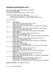
April 2007 SPECIES TRAITS IN FRAGMENTED LANDSCAPES967FIG. 1.Distribution of the studied dry grasslands in the landscape.In this study, we take into account all the abovementionedissues and ask the following questions: (1)What is the effect of dispersal and growth related traitsfor current species distribution in a landscape? (2) Howdo the conclusions of the study change when applyingphylogenetic correction? (3) How do the conclusionsdepend on the way of defining habitat isolation?To address these questions, we selected 30 speciesforming pairs of congeneric species occurring infragmented dry grasslands, a habitat not usuallyconsidered in studies of this type. We measured traitsrelated to dispersal, individual survival and growth inthe species and recorded distribution of the species in215 grassland fragments.METHODSStudy area and speciesThis study was carried out in northern Bohemia,Czech Republic. The study area is delimited by the LabeRiver on the south and by the villages of Sˇtětí, Krˇesˇice uLitomeˇrˇic, and Tuhanˇ aU´ sˇteˇk. In this region, calcareousdry grasslands form distinct localities surroundedmainly by agricultural fields (see Plate 1). A total of215 dry grasslands were mapped representing all drygrassland localities within a region of approximately 40km 2 (Fig. 1). A locality is defined as a continuousgrassland with visually homogenous vegetation separatedfrom other localities by an unsuitable area. In cases ofabrupt vegetation change within continuous grassland,the parts with different vegetation were treated asdifferent localities. These cases were not common; inall of them there was a visual topographic barrierbetween the localities such as a small ditch or change ofslope from very steep to flat.We selected 30 native perennial herbs that wererestricted to dry calcareous grasslands in the studyregion and that are neither very rare nor extremelycommon in these localities. The species were alsoselected to form 15 pairs of closely related species(Table 1). While most pairs consisted of species of thesame genus, in four cases, the pairs consisted ofrelatively closely related species from the same family(Table 1). To explore the effect of these four moredistantly related species pairs on the conclusions, wecarried all analyses both with and without them.Species traitsWe measured two types of traits: traits related tospecies dispersal ability and traits related to speciessurvival and growth. They were terminal velocity, plantheight, ability to attach to sheep fur (exozoochory), seedmass, seed production, seed germination, proportion ofviable seeds, seed dormancy, ability to flower in the firstyear (early flowering), production of aboveground and

968 KATEŘINA TREMLOVÁ AND ZUZANA MU¨ NZBERGOVÁ Ecology, Vol. 88, No. 4belowground biomass within one field season, andsurvival in the seed bank.Terminal velocity was estimated by measuring theflight time of a seed from a predefined height (3 m;Mu¨nzbergova´ 2004). Ten seeds from each of threedifferent populations of each species were measured.The type of propagule used for the measurementscorresponded to the propagule leaving the plant. Meandispersal distance (D, referred to as anemochory) wasexpressed asD ¼ðw 3 hÞ=tð1Þwhere w is the wind speed, h is the plant height, and t isthe terminal velocity. The wind speed used for thecalculation was a maximum daily mean wind speeddetected at a nearby meteorological station (Doksany)between 1993 and 2003 (13.7 m/s). This value wasselected just to illustrate the possible consequences of theterminal velocity and plant height for seed dispersal.Since wind speed is a constant in the calculation, usingother values would not affect the results. Plant heightwas estimated by measuring the height of 10 randomlyselected flowering plants per locality at each of threeselected localities.We are aware that our dispersal model is verysimplified. Nevertheless, it has been successfully usedin other studies to characterize mean dispersal distanceof seeds (e.g., Soons and Heil 2002, Mu¨nzbergová et al.2005, Herben et al. 2006) and is the easiest way tocombine the three key parameters affecting dispersal.We thus suggest that it is a useful proxy of potentialwind dispersal distances for comparison among thespecies.Ability to disperse via exozoochory was assessed bygently placing a piece of sheep fur over a tray containing100 seeds, removing it and counting the number ofattached seeds (Mu¨nzbergova´ 2004).Seed mass was estimated by weighing five groups of 10seeds from three source populations. It is generallyrecognized that seed mass can serve as proxy of seeddispersal ability and germination as well as competitiveability of the species.Seed production was estimated as number of floweringplants per square meter counted in 10 quadrats ineach of three populations of the species. The quadratswere intentionally selected in areas with the highestdensity of the species that could be found in the differentpopulations. This number was multiplied by seedproduction per plant estimated in these populations.This value was then multiplied by the proportion ofviable seeds to estimate number of viable seeds producedper area per year. This value provides information onmaximum seed production by a stand of a given species.It thus provides an estimate of the potential supply ofseeds ready to colonize other localities.Traits related to plant growth were estimated in acommon garden experiment. In late summer (August toSeptember) 2003, 50 seeds of a single species were sownTABLE 1.List of species used in the study.Pairno.Species Abbreviation Family1 Agrimonia eupatoria Agr eup RosaceaeSanguisorba minor San min Rosaceae2 Asperula cynanchica Asp cyn RubiaceaeAsperula tinctoria Asp tin Rubiaceae3 Astragalus cicer Ast cic LeguminosaeAstragalus glycyphyllos Ast gly Leguminosae4 Brachypodium pinnatum Bra pin GramineaeBromus erectus Bro ere Gramineae5 Campanula glomerata Cam glo CampanulaceaeCampanula rotundifolia Cam rot Campanulaceae6 Carex tomentosa Car tom CyperaceaeCarex flacca Car fla Cyperaceae7 Centaurea jacea Cen jac CompositaeCentaurea scabiosa Cen sca Compositae8 Cirsium acaule Cir aca CompositaeCirsium pannonicum Cir pan Compositae9 Coronilla vaginalis Cor vag LeguminosaeCoronilla varia Cor var Leguminosae10 Inula hirta Inu hir CompositaeInula salicina Inu sal Compositae11 Laserpitium latifolium Las lat UmbelliferaePeucedanum cervaria Peu cer Umbelliferae12 Linum flavum Lin fla LinaceaeLinum tenuifolium Lin ten Linaceae13 Lotus corniculatus Lot cor LeguminosaeMedicago falcata Med fal Leguminosae14 Salvia pratensis Sal pra LabiataeSalvia verticillata Sal ver Labiatae15 Trifolium medium Tri med LeguminosaeTrifolium montanum Tri mon LeguminosaeNote: The nomenclature follows Tutin et al. (1964–1983).in 19 3 19 3 19 cm pots in a common garden in a 1:2mixture of sand and garden substrate. For each species,seeds originating from three different localities wereused. Seeds from one locality were placed into one pot;there were three replicates per locality and species thusyielding nine pots per species.In November 2003, we recorded the number ofgerminated seedlings per pot. Since the species eithergerminated at a high rate in the autumn or did notgerminate at all, we coded this information as a binaryvariable (dormancy; yes or no). The ability to germinateearly indicates that the seeds do not posses any type ofdormancy. For determining seed dormancy, it isimportant that the seeds be sown shortly after beingharvested. This information provides an indication ofthe germination dynamics of the species and thus aboutthe potential performance of the seedlings at thelocalities.The number of plants in the pot was also recorded inMay 2004 for all species to have the same recording datefor species with and without seed dormancy. For theearly germinating species, the May germination was thenumber of germinated plants in autumn reduced bywinter mortality. This number served as an estimate ofgermination fraction (germination in Petri dishes wasused only to estimate production of viable seeds perarea).

April 2007 SPECIES TRAITS IN FRAGMENTED LANDSCAPES969TABLE 2.List of traits used in the study.ParameterUnitsSeed massmgTerminal velocity m/sAnemochorymean dispersal distance (m)Seed production viable seeds/m 2Seed bank 100 (percentage decline ingermination ability after 1 yr)Exozoochory seeds attached to sheep fur (%)Germination fractionà plants after 1 yr from sown seeds(%)Dormancy ,à0/1 (germination in autumn/spring)Early flowering ,à 1/0 (flowering in the first year)Aboveground biomass ,à g (for one plant after 1 yr)These parameters were used in the test presented in thisstudy.à These parameters come from the common garden experiment.In autumn (September–November) 2004, we recordedthe presence of flowering plants in the pots to assess theability of the species to flower in the first year (earlyflowering; yes or no). In November 2004, the plants wereharvested. Each harvested plant was divided into aboveandbelowground biomass, dried to constant mass, andweighed. We used the mass of the largest plant perspecies as an estimate of growth ability of the species; inall cases there were one to three large plants in the potand sometimes also many small ones. We suggest thatthe size of the largest plant provides a relatively goodestimate of what a plant can do in natural conditionswithin one year. This indicates that the flowering canalso be interpreted as the ability of the species to do so,since at least some plants did not suffer from highcompetition. The division of the species into early andlate flowering categories, and biomass production of theplant, correspond well with our personal observationson performance of the plants in the field. We thussuggest these data can provide insights into growthdynamics of the plants in the field.To estimate the ability to survive in the seed bank,three nylon bags per species, each containing 50 seeds,were buried at each of two different localities inNovember 2003 and excavated in October 2004. Theexcavated seeds were tested for viability. The seeds wereregularly watered with distilled water on the Petri dishesand kept in a growth chamber under a fluctuatingregime (12 hours light at 208C, 12 hours dark at 108C).Germinated seeds were regularly removed. The seeds ofspecies that did not germinate were stimulated by addinggiberelic acid and abraded by sandpaper. The seeds thatstill did not germinate and did not decay were thentested for viability using the tetrazolium test. All seedsidentified as viable by any of the methods were summed.The same procedure was used to estimate the viability offresh seeds (proportion of viable seeds) to provide abaseline from which to estimate the decline in germinationover time. The ability to form a seed bank indicatesthat the seed can survive given that it does not havesuitable conditions for germination. It, however, doesnot imply it has any intrinsic dormancy.All measured traits are listed in Table 2 and values ofthese traits for each species are in Appendix A. In allcases, we were working with average values for eachspecies.Habitat suitabilityTo calculate habitat occupancy and isolation of ahabitat, we had to define suitable localities. Suitablelocalities were defined using a Beals index (Beals 1984,Mu¨nzbergova´ and Herben 2004). This index calculatesthe probability of encountering a species at a localityusing data on the presence of other species at thatlocality and on patterns of co-occurrence of the targetspecies with other species. To estimate the species cooccurrencepatterns, we used 2984 releve´s on speciescomposition of dry calcareous grasslands in the CzechRepublic from the Czech national phytosociologicaldatabase (Chytrý and Rafajova´ 2003). Unoccupiedlocalities with a Beals index reaching at least the 5%quantile of the Beals index of occupied localities wereconsidered suitable. Using 1% or 10% quantiles did notsignificantly affect the conclusions.We also used data on abiotic conditions of thelocalities (geology, potential direct solar radiation, andslope of the target localities) to assess habitat suitability.These gave very similar results to the Beals index, so weuse only the former in the study.Habitat isolationWe used three different approaches to calculatehabitat isolation in this study. First, we calculatedisolation of a locality using its distance from all drygrasslands, subjectively assumed to be suitable for all thespecies, in the study region. In this case, habitat isolationof a given locality was the same for all the species.Second, we calculated isolation only from all occupiedlocalities. In this and in the following case, habitatisolation of a single locality differed among species.Finally, we calculated isolation from all localitiesclassified as suitable for the species using the Bealsindex. See Introduction for the rationale behind calculatingisolation from unoccupied localities and Eq. 2 forthe exact way to do this.Calculation of habitat isolation was based oncentroids of the localities, derived from a digital mapof the localities provided by T. Chýlova´. Isolation of alocality was expressed as a mass of surroundinglocalities weighted by its distance to the target locality.Isolation of a locality was expressed as follows:I ij ¼ X h inP k =djk2 3 O k ; j 6¼ k ð2Þk¼1where I ij is isolation of locality j for species i, k are all thesurrounding localities within 1.8 km distance from thetarget locality, P k is a size of locality k in squarekilometers, d jk is distance between localities j and k in

970 KATEŘINA TREMLOVÁ AND ZUZANA MU¨ NZBERGOVÁ Ecology, Vol. 88, No. 4TABLE 3.Correlations among single traits used in the study.ParameterSeedmassAnemochorySeedproductionDormancyEarlyfloweringAbovegroundbiomassSeedbankExozoochoryWithout phylogenetic correctionSeed mass 0.135 0.127 0.073 0.066 0.233 0.118 0.104Anemochory 0.135 0.050 0.193 0.181 0.273 0.106 0.475Seed production 0.127 0.050 0.254 0.091 0.091 0.266 0.312Germination fraction 0.153 0.147 0.216 0.117 0.177 0.215 0.180 0.079Dormancy 0.073 0.193 0.254 0.391 0.258 0.103 0.248Early flowering 0.066 0.181 0.091 0.391 0.498 0.122 0.129Aboveground biomass 0.233 0.273 0.091 0.258 0.498 0.653 0.375Seed bank 0.118 0.106 0.266 0.103 0.122 0.653 0.500Exozoochory 0.104 0.475 0.312 0.248 0.129 0.375 0.500With phylogenetic correctionSeed mass 0.069 0.052 0.342 0.125 0.326 0.293 0.488Anemochory 0.069 0.066 0.174 0.056 0.050 0.205 0.199Seed production 0.052 0.066 0.317 0.142 0.257 0.413 0.057Germination fraction 0.312 0.144 0.133 0.428 0.405 0.068 0.149 0.134Dormancy 0.342 0.174 0.317 0.589 0.186 0.100 0.081Early flowering 0.125 0.056 0.142 0.589 0.286 0.159 0.006Aboveground biomass 0.326 0.050 0.257 0.186 0.286 0.390 0.571Seed bank 0.293 0.205 0.413 0.100 0.159 0.390 0.278Exozoochory 0.488 0.199 0.057 0.081 0.006 0.571 0.278Notes: Significant correlations (P , 0.05) are in boldface. No correction for multiple testing was used here.kilometers, and O k is a binary (0,1) variable codingoccupancy or suitability of a locality. When calculatingisolation from all localities, O k is always 1.Isolation of a locality was calculated only for 187localities out of 215. The other localities were excludedbecause there were unanalyzed localities within 1.8 kmof these localities. The 1.8-km zone was selected as adistance over which habitat isolation was measured; thiswas the maximum distance that we were able to reliablycover by the field survey. Not all marginal localities hadto be excluded, however, since large areas of arable fieldssurrounded some of the localities. Only the 187 localitieswere used in all the subsequent analyses.Data analysisTo reduce the high dimensionality of the trait-byspeciesmatrix, we selected only a subset of traits thatwere expected to be most informative and not tooclosely correlated with other traits (Table 2). Correlationof the remaining species traits was studied using simplecorrelation analysis. The traits that changed values overseveral orders of magnitude (seed mass, seed production,aboveground biomass) were logarithmically transformedbefore the analysis. This analysis was thenrepeated after subtracting the mean trait value for eachspecies pair from the trait value of each species in thatpair; this was done to explore correlation among traitsafter phylogenetic correction.Some traits used in the analysis were significantlycorrelated (Table 3), but we did not want to excludethose since they carry different biologically meaningfulinformation. In all the subsequent analyses, we werethus using multiple partly correlated traits. This couldtheoretically bias our conclusions. To explore this, we inall cases compared a test with all the variables includedwith results of stepwise analysis.To visualize similarity between the different species intheir traits we used principal component analysis (PCA).The data on single species traits were treated as‘‘species,’’ and data on each species represented ‘‘samples.’’The analysis was centered and standardized by‘‘species’’; in this way all the traits were expressed in thesame, relative, units. For this as well as for subsequentanalyses, we used only traits marked in Table 2.Percentage of occupancy of the localities was expressedas the portion of all occupied localities eitherfrom all localities, or from all suitable localities. Toestimate the effect of plant traits on overall habitatoccupancy, we used generalized linear models (GLM),assuming binomial distribution of the dependent variable.Numbers of occupied and all available localitieswere used as bind dependent variables (the variableswere combined into one variable using command cbindin S-PLUS 2000 (MathSoft, Needham, Massachusetts,USA), the resulting variable carries information onfrequency of an event), and all species traits were used asindependent variables. The same analysis was thenrepeated with pair code as another independent variable.To estimate the effect of species traits and landscapeproperties on species occurrence at a locality, we usedlogistic regression. Presence of each species in eachlocality was used as the dependent variable, and size andisolation of a locality, all species traits, and theinteraction of all species traits with habitat size andisolation were used as independent variables. In the text,however, we present only the results for the interactionterms of habitat isolation/size and species traits. Theresults of the main effects would actually be a more

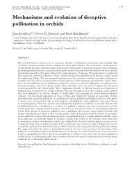
April 2007 SPECIES TRAITS IN FRAGMENTED LANDSCAPES971FIG. 2. Relationship between individual species determined by principal component analysis (PCA) using trait data asdependent variables. Species with solid black symbols are from the family Leguminosae, species with solid gray symbols are fromthe family Compositae, and species with open symbols are from the other families (each of these pairs is from a different family).Species abbreviations are provided in Table 1.complicated approach to study the effect of traits onhabitat occupancy mentioned above.Analyses calculating isolation from all dry grasslandsin the region and from only occupied localities werebased on all the studied localities. In the analyses withisolation calculated from all suitable localities, we usedata only from suitable localities for each species.To visualize interactions of traits and landscapeproperties in a graphic form, we plotted the traits forspecies occurring in localities with a given propertyagainst the property. The species missing at each localitywere not visualized in these graphs. To visualize theresults after phylogenetic correction, we used speciestraits after subtracting the mean of the trait value foreach species pair from the trait value.All the above analyses are based on traits across all 30species and do not allow easy interpretation of thedistribution of the single species. To show how singlespecies respond to habitat size and isolation, weperformed a multivariate canonical correspondenceanalysis (CCA) using presence of all the species at thelocality (species composition based on the 30 species) asthe dependent variable and habitat size or isolation asindependent variables. To separate the effect of habitatsize and isolation, we also performed analyses withhabitat size as an independent variable and isolation ascovariate and the other way round. The analyses weredone only for isolation from all localities, i.e., the type ofisolation that is the same for all the species.All the univariate analyses were done using S-PLUS2000; all the multivariate analyses were done usingCANOCO (ter Braak and Sˇmilauer 1998). All theunivariate analyses were done with type III sum ofsquares, so the effect of each independent variable wasestimated after removing the effect of all the otherindependent variables.RESULTSCorrelation of the different traits shows a positiverelationship between anemochory and exozoochory.There is also a positive relationship between abovegroundbiomass of a plant in the first year and its abilityto flower in the first year and to produce a seed bank.Plants with high aboveground biomass tend to have lowability to disperse via exozoochory. There is also anegative relationship between ability to create seed bankand exozoochory and between seed dormancy andability to flower early (Table 3).Only three of these relationships stay significant afterphylogenetic correction (between aboveground biomassand seed bank and exozoochory and between earlyflowering and dormancy). There is also a significantpositive relationship between seed mass and exozoochoryand seed production and seed bank (Table 3). Thecorrelations partly change after removing the four noncongenericpairs (see Appendix B).Comparison of traits of species within the pairsindicates that many species within a pair are ratherdissimilar (Fig. 2). Nevertheless, species pair explains78% of the total variation in the dataset as identifiedusing PCA with species pair as a covariate.Tests exploring the effect of species traits on habitatoccupancy indicate many significant patterns (Table 4).When working with all localities and without phyloge-

April 2007 SPECIES TRAITS IN FRAGMENTED LANDSCAPES973Effects of interactions between habitat size/isolation and species traits on species occurrence at a locality estimated usinglogistic regression.TABLE 5.Without PCWith PCHabitat size Isolation Habitat size IsolationParametersP R 2 P R 2 P R 2 P R 2Occupied localitiesSeed mass 0.895 0.05 0.005 ( ) 0.384 0.01 0.002 (þ)Anemochory 0.622 ,0.001 0.006 ( ) 0.584 ,0.001 0.006 ( )Seed production 0.32 0.178 0.666 0.749Dormancy 0.337 0.001 0.002 (þ) 0.524 0.236Early flowering 0.049 0.001 ( ) ,0.001 0.003 (þ) 0.401 0.13Aboveground biomass 0.441 0.004 0.002 (þ) 0.978 ,0.001 0.002 ( )Seed bank 0.281 0.024 0.001 (þ) ,0.001 0.003 (þ) 0.022 0.002 (þ)Exozoochory 0.736 0.56 0.384 0.35All localitiesSeed mass 0.424 0.941 0.049 0.001 (þ) 0.854Anemochory 0.437 0.107 0.344 0.078 0.001 ( )Seed production 0.286 0.509 0.682 0.789Dormancy 0.228 0.456 0.405 0.601Early flowering 0.05 0.001 ( ) 0.733 0.445 0.558Aboveground biomass 0.341 0.117 0.995 0.114Seed bank 0.251 0.14 0.086 0.001 (þ) 0.065 0.001 (þ)Exozoochory 0.707 0.522 0.381 0.578Suitable localitiesSeed mass 0.446 0.776 0.049 0.001 (þ) 0.46Anemochory 0.244 0.001 0.002 (þ) 0.396 0.003 0.002 ( )Seed production 0.238 0.3 0.525 0.434Dormancy 0.829 0.508 0.71 0.796Early flowering 0.239 0.381 0.693 0.488Aboveground biomass 0.535 0.152 0.977 0.234Seed bank 0.228 0.092 0.086 0.047 0.001 (þ)Exozoochory 0.809 0.3 0.383 0.193Notes: The sign of the relationship is provided for significant results. Error df ¼ 3707 and 3692 for analyses using isolation fromall or occupied localities without and with phylogenetic correction (PC), respectively; error df ¼ 3274 and 3259 for analyses usingisolation from all suitable localities without and with phylogenetic correction, respectively.covariate did not change these results very much andthus are not shown. In more isolated localities, speciessuch as Inula hirta, Campanula rotundifolia, Cirsiumacaule, Salvia pratensis, and Astragalus glycyphyllos aremore common. On the other hand, species such asLinum flavum, Laserpitium latifolium, Cirsium pannonicum,Coronilla vaginalisi, and Campanula glomerata aremore common in less isolated localities (see Table 6 forfull list of species). Smaller localities host species such asCampanula glomerata, Laserpitium latifolium, Bromuserectus, and Cirsium pannonicum, while in largerlocalities Inula hirta, Linum tenuifolium, Campanularotundifolia, and Asperula tinctoria are more common(see Table 5 for a full list of species). These relationshipsdid not change much after removing the non-congenericpairs. The main difference was a lower percentage ofvariation explain by habitat size and isolation (notshown).DISCUSSIONResults of this study show a strong relationshipbetween species traits and species distribution in thelandscape. This is true both when looking at percentageof habitat occupancy and when looking at speciesresponse to habitat size and isolation. However, thespecific nature of the relationships often changes afterphylogenetic correction or with different definitions ofhabitat isolation.Exploration of species traits studied in this paperindicates many significant relationships between these.For example, we have demonstrated significant relationshipbetween the ability to disperse by anemochoryand exozoochory (see also Fischer et al. 1996). Ourresults, however, also indicate that this pattern disappearswhen performing phylogenetic correction. Similarly,we found a negative relationship between seeddispersal ability (exozoochory) and survival in the seedbank (see also Ehrle´n and Groenendael 1998). Again,this relationship disappeared after phylogenetic correction.The reversal of the relationships between speciestraits after phylogenetic correction is in agreement withprevious studies (e.g., Silvertown and Dodd 1996) andsuggests that we should expect different conclusions inthe subsequent analyses with and without phylogeneticcorrection.Percentage of habitat occupancy was significantlyaffected by both traits related to seed dispersal and traitsrelated to plant growth. A high number of species traitsexplaining habitat occupancy is in agreement withprevious studies exploring this relationship (e.g., Ouborg

974 KATEŘINA TREMLOVÁ AND ZUZANA MU¨ NZBERGOVÁ Ecology, Vol. 88, No. 4FIG. 3. Relationship between species traits and landscapeproperties: (A) anemochory and habitat isolation, (B) log(seedmass) and habitat isolation, and (C) log(seed mass) afterphylogenetic correction and habitat isolation. For the purposeof the graph, habitat isolation was divided into threeequidistant categories. In each case, only species occurring atthe given locality are included. All the patterns are significant(Table 5).1993, Eriksson and Jakobsson 1998, Maurer et al. 2003,Kolb and Diekmann 2005). In our study, more widelydistributed species had better dispersal ability as well asfaster growth. Kolb and Diekmann (2005) found asimilar pattern for dispersal. On the other hand,Eriksson and Jakobsson (1998) and Maurer et al.(2003) have shown that habitat occupancy does notdepend on traits related to dispersal.Species traits also determine species response tohabitat size and isolation; with more significant interactionswith habitat isolation than with size. This is inagreement with conclusions of Piessens et al. (2004) andKolb and Diekmann (2005), who showed higher effectsof habitat isolation than size on species occurrence inforest fragments. In all comparisons, we have shownthat species with higher anemochory are missing fromisolated localities. This contrasts with conclusions ofPiessens et al. (2005), who suggested that anemochory isthe most important trait allowing species survival atisolated localities. The observed pattern clearly indicatesthat anemochory is not the main factor that canguarantee species occurrence in isolated localities. Alsowe did not find any significant effect of exozoochory.This may indicate that it is not dispersal but ratherestablishment that limits species distribution at isolatedhabitats. It is, however, also possible that other dispersaltraits that were not measured in this study, such asendozoochory, are the most important dispersal types inthe studied landscape (e.g., Bonn 2004). Isolatedlocalities also host species with significantly smallerseeds suggesting that seed size might be better predictorof dispersal than our (assumed) more direct measures ofdispersability (Ehrle´n and Eriksson 2000).In agreement with Piessens et al. (2004), we haveshown that survival in the seed bank is important forspecies presence in isolated localities. This pattern is alsoin agreement with many other studies that indicate thatsurvival in seed bank is crucial for population survival(e.g., Thompson et al. 1998, Turnbull et al. 2000).The results also show that species occurring in smallerlocalities flower earlier than species in larger localities.This can be explained by the fact that small localitieshave a higher edge-to-area ratio and are thus moredisturbed. Disturbed localities have also been shown tohost early flowering species in previous studies (e.g.,Thompson and Rabonowitz 1989, Thompson andHodkinson 1998, Silvertown and Charlesworth 2001,Ehrle´n and Lehtilä 2002).An important conclusion from this study is that theeffect of species traits on species response to habitat sizeand isolation can completely reverse when applyingphylogenetic correction (reversals after phylogeneticcorrection were found also by Murray et al. [2002] andPocock et al. [2006] but not, e.g., by Maurer et al. [2003]and De Bello et al. [2005]). For example, species weredetected to have smaller seeds when occurring at moreisolated localities, but this relationship reversed directionafter phylogenetic correction (see also Eriksson andJakobsson 1998). The contradiction between the twopatterns is probably a consequence of the stability ofseed size within species phylogenies (e.g., Mazer 1989,Kelly and Purvis 1993, Kelly 1995). The main effect ofseed size was thus probably removed when performing

April 2007 SPECIES TRAITS IN FRAGMENTED LANDSCAPES975Response of studied species to habitat isolation and size determined using canonicalcorrespondence analysis (CCA).TABLE 6.Response to isolationResponse to habitat sizeSpecies Position Species PositionInula hirta 0.402 Campanula glomerata 0.6187Campanula rotundifolia 0.2091 Laserpitium latifolium 0.6081Cirsium acaule 0.1722 Bromus erectus 0.1377Salvia pratensis 0.1411 Cirsium pannonicum 0.127Astragalus glycyphyllos 0.1187 Linum flavum 0.0943Bromus erectus 0.1017 Sanguisorba minor 0.0753Carex tomentosa 0.0655 Brachypodium pinnatum 0.0681Trifolium medium 0.0629 Salvia verticillata 0.0597Asperula tinctoria 0.0604 Coronilla varia 0.0585Lotus corniculatus 0.0503 Centaurea jacea 0.0429Carex flacca 0.0404 Agrimonia eupatoria 0.0162Agrimonia eupatoria 0.0139 Asperula cynanchica 0.0024Centaurea scabiosa 0.0037 Trifolium montanum 0.0091Coronilla varia 0.0111 Lotus corniculatus 0.0094Brachypodium pinnatum 0.0215 Cirsium acaule 0.0142Medicago falcata 0.0276 Medicago falcata 0.016Sanguisorba minor 0.0384 Carex flacca 0.0305Trifolium montanum 0.0457 Trifolium medium 0.0382Centaurea jacea 0.0591 Coronilla vaginalis 0.0447Salvia verticillata 0.0601 Centaurea scabiosa 0.0562Linum tenuifolium 0.0664 Salvia pratensis 0.0612Inula salicina 0.1001 Inula salicina 0.0694Astragalus cicer 0.1112 Carex tomentosa 0.0737Asperula cynanchica 0.1184 Astragalus glycyphyllos 0.1182Peucedanum cervaria 0.3271 Astragalus cicer 0.1682Campanula glomerata 0.3499 Peucedanum cervaria 0.1968Coronilla vaginalis 0.363 Asperula tinctoria 0.2291Cirsium pannonicum 0.7953 Campanula rotundifolia 0.2575Laserpitium latifolium 0.8394 Linum tenuifolium 0.3596Linum flavum 1.0103 Inula hirta 0.6533Notes: Habitat isolation explained 9.02% of the variation in species composition that could beexplained by one ordination axis; the effect is significant. Habitat size explained 6.01% of thevariation in species composition that could be explained by one ordination axis; the effect ismarginally significant. The table shows position on the first ordination axis; negative values indicatespecies prevailing at isolated and small localities, respectively.the analysis of phylogenetically contrasting pairs. Theresidual variation in seed size may describe differences inspecies ability to establish at these localities (reserveeffect [Westoby et al. 1996]) given that they dispersethere.The potential reversal of conclusions after applicationof phylogenetic correction indicates that interpretationof the results of previous studies on this topic (e.g.,Ouborg 1993, Quintana-Ascentio and Menges 1996) interms of factors responsible for species distribution inthe landscape is partly problematic. Since these studiesusually do not perform the phylogenetic correction, it isnot clear which patterns are really the effects of the giventrait and which are just due to other correlatedproperties of the whole genus. On the other hand, evenresults with phylogenetic correction have to be interpretedwith caution since we may miss patterns that arecharacteristic for the whole species group. Both types ofrelationship should thus be explored to understandspecies-traits–landscape-structure relationships.The results also show strong differences in conclusionswhen working with different isolation measures. Thehighest number of significant relationships was foundwhen working with isolation calculated from occupiedlocalities only; this model thus has the best predictiveability for species distribution. This is a measure that hasbeen previously used by others (e.g., Quintana-Ascentioand Menges 1996, Johansson and Ehrle´n 2003, Hanskiet al. 2004). Its significance suggests that it is currentlandscape occupancy, and not distribution of suitablelocalities in the landscape, that determines the probabilityof species occurrence on single localities. Whileboth conclusions would be compatible with the predictionsof metapopulation theory (e.g., Hanski 1999), wesuggest that higher predictive power of a modelmeasuring isolation from occupied localities indicatesrelatively slow dynamics of the species.The analysis of effect of habitat size and isolation onspecies composition of the locality confirms that habitatisolation is more important than habitat size. The groupof species restricted to non-isolated localities includesmany endangered species such as Linum flavum, Cirsiumpannonicum, and Coronilla vaginalis. This indicates thathabitat fragmentation constitutes a serious threat to drygrassland species in the region.In this paper, we have explored the effect of speciestraits on species distribution in the current landscape asdescribed by current habitat size and isolation. It has,

976 KATEŘINA TREMLOVÁ AND ZUZANA MU¨ NZBERGOVÁ Ecology, Vol. 88, No. 4however, been repeatedly shown that species distributionmay depend not only on current landscapestructure, but also on landscape structure in the past(Jacquemyn et al. 2001, Johansson and Ehrle´n 2003,Lindborg et al. 2005, Herben et al. 2006). However,exploring the effect of past landscape structure wasbeyond the scope of the current study.ConclusionsWe have shown many significant relationships betweenspecies traits related to both dispersal and growth andspecies distribution in the landscape. The directions ofthese relationships, however, often change after applicationof phylogenetic correction. The conclusions alsopartly change depending on whether isolation is calculatedfrom all potential localities or occupied localities.All this indicates that species traits have a high potentialto explain the pattern of species distribution in thelandscape. To build predictive models of species distribution,however, we have to carefully consider thetechnique used. We suggest that the results withoutphylogenetic correction can be better used for predictingpatterns of distribution for large species groups. Thephylogenetically corrected results might be more suitablefor predicting selection pressures on changes of lifehistory traits within smaller species groups. It has to be,however, kept in mind that the results are complementaryand both of these should be carefully considered whentrying to understand species distributions.All the results suggest also that when comparingrelationships between species traits and species distributionamong published studies we have to carefullyconsider the technique used in each particular case. Inthe future we should thus attempt to use analysis bothwith and without phylogenetic correction and exploredifferent isolation measures whenever possible and try toidentify the differences in conclusions between these.ACKNOWLEDGMENTSWe thank to Tereza Chýlova´ for help with collecting fielddata; Tomásˇ Herben, Johan Ehrlén, and Deborah E. Goldbergfor comments on the manuscript; and Deborah E. Goldberg forlanguage revision. This study was supported by GAAV grantB601110634. It was also partly supported by MSMT0021620828 and AV0Z6005908.LITERATURE CITEDAckerman, J. D., A. Sabat, and J. K. Zimmerman. 1996.Seedling establishment in an epiphytic orchid: an experimentalstudy of seed limitation. Oecologia 106:192–198.Bastin, L., and C. D. Thomas. 1999. The distribution of plantspecies in urban vegetation fragments. Landscape Ecology14:493–507.Beals, E. W. 1984. Bray-Curtis ordination: an effective strategyfor analysis of multivariate ecological data. Advances inEcological Research 14:1–55.Bonn, S. 2004. Dispersal of plants in the Central Europeanlandscape: dispersal processes and assessment of dispersalpotential exemplified for endozoochory. Dissertation zurErlangung des Doktorgrades der Naturwissenschaften,Universita¨t Regensburg, Germany.Chytrý, M., and M. Rafajová. 2003. Czech national phytosociologicaldatabase: basic statistics of the available vegetation-plotdata. Preslia 75:1–15.De Bello, F., J. Lepš, and M. T. Sebastia. 2005. Predictive valueof plant traits to grazing along a climatic gradient in theMediterranean. Journal of Applied Ecology 42:824–833.Dupré, C., and J. Ehrlén. 2002. Habitat configuration, speciestraits and plant distributions. Journal of Ecology 90:796–805.Ehrlén, J., and O. Eriksson. 2000. Dispersal limitation andpatch occupancy in forest herbs. Ecology 81:1667–1674.Ehrlén, J., and K. Lehtilä. 2002. How perennial are perennialplants? Oikos 98:308–322.Ehrlén, J., and J. M. van Groenendael. 1998. The trade-offbetween dipersability and longevity: an important aspect ofplant species diversity. Applied Vegetation Science 1:29–36.Eriksson, O. 1996. Regional dynamics of plants: a review ofevidence for remnant, source–sink and metapopulations.Oikos 77:248–258.Eriksson, O., and J. Ehrlén. 1992. Seed and microsite limitationof recruitment in plant populations. Oecologia 91:360–364.Eriksson, O., and J. Ehrle´n. 2001. Landscape fragmentationand the viability of plant populations. Pages 157–175 in J.Silvertown and J. Antonovics, editors. Integrating ecologyand evolution in a spatial context. Blackwell, Oxford, UK.Eriksson, O., and A. Jakobsson. 1998. Abundance, distributionand life histories of grassland plants: a comparative study of81 species. Journal of Ecology 86:922–933.Fischer, S. F., P. Poschlod, and B. Beinlich. 1996. Experimentalstudies on the dispersal of plants and animals on sheep incalcareous grasslands. Journal of Applied Ecology 33:1206–1222.Freckleton, R. P., P. H. Harvey, and M. Pagel. 2002.Phylogenetic analysis and comparative data: a test andreview of evidence. American Naturalist 160:712–726.Grashof-Bokdam, C. 1997. Forest species in an agriculturallandscape in the Netherlands: effects of habitat fragmentation.Journal of Vegetation Science 8:21–28.Grime, J. P., and J. G. Hodgson. 1987. Botanical contributionsto contemporary ecological theory. New Phytologist 106:283–295.Hanski, I. 1999. Metapopulation ecology. Oxford UniversityPress, New York, New York, USA.Hanski, I., C. Eralahti, M. Kankare, O. Ovaskainen, and H.Siren. 2004. Variation in migration propensity amongindividuals maintained by landscape structure. EcologyLetters 7:958–966.Harvey, P. H., A. F. Read, and S. Nee. 1995. Why ecologistsneed to be phylogenetically challenged. Journal of Ecology83:535–536.Herben, T., Z. Mu¨nzbergová, M. Mildén, J. Ehrlén, S. O. A.Cousins, and O. Eriksson. 2006. Long-term spatial dynamicsof Succisa pratensis in a changing rural landscape: linkingdynamical modeling with historical maps. Journal of Ecology94:131–143.Higgins, S. I., J. S. Clark, R. Nathan, T. Hovestadt, F. Schurr,J. M. V. Fragoso, M. R. Aguiar, E. Ribbens, and S. Lavorel.2003. Forecasting plant migration rates: managing uncertaintyfor risk assessment. Journal of Ecology 91:341–347.Jackel, A. K., and P. Poschlod. 2000. Persistence or dispersal:Which factors determine the distribution of plant species?Zeitschrift fu¨r Ökologie und Naturschutz 9:99–107.Jacquenym, H., J. Butaye, and M. Hermy. 2001. Forest plantspecies richness in small fragmented mixed deciduous forestpatches: the role of area, time and dispersal limitation.Journal of Biogeography 28:801–812.Johansson, P., and J. Ehrle´n. 2003. Influence of habitatquantity, quality and isolation on the distribution andabundance of two epiphytic lichens. Journal of Ecology 91:213–221.

April 2007 SPECIES TRAITS IN FRAGMENTED LANDSCAPES977Kelly, C. K. 1995. Seed size in tropical trees: a comparativestudy of factors affecting seed size in Peruvian angiosperms.Oecologia 102:377–388.Kelly, C. K., and A. Purvis. 1993. Seed size and establishmentconditions in tropical trees: on the use of taxonomicrelatedness in determining ecological patterns. Oecologia94:356–360.Kolb, A., and M. Diekmann. 2005. Effects of life-history traitson responses of plant species to forest fragmentation.Conservation Biology 19:929–938.Lindborg, R., S. A. O. Cousins, and O. Eriksson. 2005. Plantspecies response to land-use change: Campanula rotundifolia,Primula veris and Rhinanthus minor. Ecography 28:29–36.Matlack, G. R. 2005. Slow plants in a fast forest: local dispersalas a predictor of species frequencies in a dynamic landscape.Journal of Ecology 93:50–59.Maurer, K., W. Durka, and J. Stöcklin. 2003. Frequency ofplant species in remnants of calcareous grassland and theirdispersal and persistence characteristics. Basic and AppliedEcology 4:307–316.Mazer, S. J. 1989. Ecological, taxonomic, and life-historycorrelates of seed mass among Indiana dune angiosperms.Ecological Monographs 59:153–175.Mu¨nzbergová, Z. 2004. Effects of spatial scale on factorslimiting species distributions in dry grassland fragments.Journal of Ecology 92:854–867.Mu¨nzbergova´, Z., and T. Herben. 2004. Identification ofsuitable unoccupied habitats in metapopulation studies usingco-occurrence of species. Oikos 105:408–414.Mu¨nzbergová, Z., M. Mildén, J. Ehrlén, and T. Herben. 2005.Population viability and reintroduction strategies: a spatiallyexplicit landscape-level approach. Ecological Applications15:1377–1786.Murray, B. R., P. H. Thrall, and B. J. Lepschi. 2002. Relatingspecies rarity to life history in plants of eastern Australia.Evolutionary Ecology Research 4:937–950.Oostermeijer, J. G. B., S. H. Luijten, and J. C. M. den Nijs.2003. Integrating demographic and genetic approaches inplant conservation. Biological Conservation 113:389–398.Ouborg, N. J. 1993. Isolation, population size and extinction:the classical and metapopulation approaches applied tovascular plants along the Dutch Rhine system. Oikos 66:298–308.Piessens, K., O. Honnay, and M. Hermy. 2005. The role offragment area and isolation in the conservation of heathlandspecies. Biological Conservation 122:61–69.Piessens, K., O. Honnay, K. Nackaerts, and M. Hermy. 2004.Plant species richness and composition of heathland relics innorthwestern Belgium: Evidence for a rescue effect? Journalof Biogeography 31:1683–1692.Pocock, M. J. O., S. Hartley, M. G. Telfer, C. D. Preston, andW. E. Kunin. 2006. Ecological correlates of range structure inrare and scarce British plants. Journal of Ecology 94:581–596.Quintana-Ascencio, P. F., and E. S. Menges. 1996. Inferringmetapopulation dynamics from patch-level incidence ofFlorida scrub plants. Conservation Biology 10:1210–1219.Reich, P. B., I. J. Wright, J. Cavender-Bares, J. M. Craine, J.Oleksyn, M. Westoby, and M. B. Walters. 2003. Theevolution of plant functional variation: traits, spectra, andstrategies. International Journal of Plant Sciences 164:143–164.Silvertown, J. W., and D. Charlesworth. 2001. Introduction toplant population biology. Osney Mead, Oxford, UK.Silvertown, J., and M. Dodd. 1996. Comparing plants andconnecting traits. Philosophical Transactions of the RoyalSociety of London, B 351:1233–1239.Soons, M. B., and G. W. Heil. 2002. Reduced colonizationcapacity in fragmented populations of wind-dispersed grasslandforbs. Journal of Ecology 90:1033–1043.ter Braak, C. J. F., and P. Sˇmilauer. 1998. CANOCO referencemanual and user’s guide to Canoco for Windows: softwarefor canonical community ordination, version 4.5. MicrocomputerPower, Ithaca, New York, USA.Thompson, K., J. P. Bakker, R. M. Bekker, and J. G. Hodgson.1998. Ecological correlates of seed persistence in soil in thenorth-west European flora. Journal of Ecology 86:163–169.Thompson, K., and D. J. Hodkinson. 1998. Seed mass, habitatand life history: a re-analysis of Salisbury 1942, 1974. NewPhytologist 138:163–167.Thompson, K., and D. Rabinowitz. 1989. Do big plants havebig seeds? American Naturalist 133:722–728.Tischendorf, L., and L. Fahring. 2000. On the usage andmeasurement of landscape connectivity. Oikos 90:7–19.Trakhtenbrot, A., R. Nathan, G. Perry, and D. M. Richardson.2005. The importance of long-distance dispersal in biodiversityconservation. Diversity and Distributions 11:173–181.Turnbull, L. A., M. J. Crawley, and M. Rees. 2000. Are plantpopulations seed-limited? A review of seed sowing experiments.Oikos 88:225–238.Tutin, T. G., V. H. Heywood, N. A. Burges, D. H. Valentine,S. M. Walters, and D. A. Webb, editors. 1964–1983. FloraEuropaea. Cambridge University Press, New York, NewYork, USA.van der Meijden, E., P. G. L. Klinkhamer, T. J. De Jong, andC. A. M. Van Wijk. 1992. Meta-population dynamics ofbiennial plants: how to exploit temporary habitats. ActaBotanica Neerlandica 41:249–270.Westoby, M., M. R. Leishman, and J. M. Lord. 1995a. Furtherremarks on phylogenetic correction. Journal of Ecology 83:727–729.Westoby, M., M. R. Leishman, and J. M. Lord. 1995b. Onmisinterpreting the phylogenetic correction. Journal ofEcology 83:531–534.Westoby, M., M. R. Leishman, and J. M. Lord. 1996.Comparative ecology of seed size and dispersal. PhilosophicalTransactions of the Royal Society of London, B 351:1309–1317.APPENDIX AValues of all the traits for all the studied species (Ecological Archives E088-060-A1).APPENDIX BCorrelation among single traits used in the study after removing the four non-congeneric species pairs (Ecological Archives E088-060-A2).