SVM Example

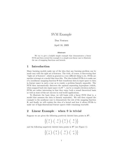
SVM ExampleDan VenturaApril 16, 2009AbstractWe try to give a helpful simple example that demonstrates a linearSVM and then extend the example to a simple non-linear case to illustratethe use of mapping functions and kernels.1 IntroductionMany learning models make use of the idea that any learning problem can bemade easy with the right set of features. The trick, of course, is discovering that“right set of features”, which in general is a very difficult thing to do. SVMs areanother attempt at a model that does this. The idea behind SVMs is to make useof a (nonlinear) mapping function Φ that transforms data in input space to datain feature space in such a way as to render a problem linearly separable. TheSVM then automatically discovers the optimal separating hyperplane (which,when mapped back into input space via Φ −1 , can be a complex decision surface).SVMs are rather interesting in that they enjoy both a sound theoretical basisas well as state-of-the-art success in real-world applications.To illustrate the basic ideas, we will begin with a linear SVM (that is, amodel that assumes the data is linearly separable). We will then expand theexample to the nonlinear case to demonstrate the role of the mapping functionΦ, and finally we will explain the idea of a kernel and how it allows SVMs tomake use of high-dimensional feature spaces while remaining tractable.2 Linear Example – when Φ is trivialSuppose we are given the following positively labeled data points in R 2 :{( ) ( ) ( ) ( )}3 3 6 6, , ,1 −1 1 −1and the following negatively labeled data points in R 2 (see Figure 1):{( ) ( ) ( ) ( )}1 0 0 −1, , ,0 1 −1 01

Figure 1: Sample data points in R 2 . Blue diamonds are positive examples andred squares are negative examples.We would like to discover a simple SVM that accurately discriminates thetwo classes. Since the data is linearly separable, we can use a linear SVM (thatis, one whose mapping function Φ() is the identity function). By inspection, itshould be obvious that there are three support vectors (see Figure 2):{s 1 =( 10), s 2 =( 31), s 3 =( 3−1In what follows we will use vectors augmented with a 1 as a bias input, andfor clarity we will differentiate these with an over-tilde. So, if s 1 = (10), then˜s 1 = (101). Figure 3 shows the SVM architecture, and our task is to find valuesfor the α i such that)}α 1 Φ(s 1 ) · Φ(s 1 ) + α 2 Φ(s 2 ) · Φ(s 1 ) + α 3 Φ(s 3 ) · Φ(s 1 ) = −1α 1 Φ(s 1 ) · Φ(s 2 ) + α 2 Φ(s 2 ) · Φ(s 2 ) + α 3 Φ(s 3 ) · Φ(s 2 ) = +1α 1 Φ(s 1 ) · Φ(s 3 ) + α 2 Φ(s 2 ) · Φ(s 3 ) + α 3 Φ(s 3 ) · Φ(s 3 ) = +1Since for now we have let Φ() = I, this reduces toα 1 ˜s 1 · ˜s 1 + α 2 ˜s 2 · ˜s 1 + α 3 ˜s 3 · ˜s 1 = −1α 1 ˜s 1 · ˜s 2 + α 2 ˜s 2 · ˜s 2 + α 3 ˜s 3 · ˜s 2 = +1α 1 ˜s 1 · ˜s 3 + α 2 ˜s 2 · ˜s 3 + α 3 ˜s 3 · ˜s 3 = +1Now, computing the dot products results in2

Figure 2: The three support vectors are marked as yellow circles.Figure 3: The SVM architecture.3

2α 1 + 4α 2 + 4α 3 = −14α 1 + 11α 2 + 9α 3 = +14α 1 + 9α 2 + 11α 3 = +1A little algebra reveals that the solution to this system of equations is α 1 =−3.5, α 2 = 0.75 and α 3 = 0.75.Now, we can look at how these α values relate to the discriminating hyperplane;or, in other words, now that we have the α i , how do we find the hyperplanethat discriminates the positive from the negative examples? It turns outthat˜w = ∑ iα i ˜s i⎛= −3.5 ⎝ 1 0⎛1⎞1= ⎝ 0 ⎠−2⎞⎠ + 0.75⎛⎝ 3 11⎞ ⎛⎠ + 0.75 ⎝ 3⎞−1 ⎠1Finally, remembering that our vectors are augmented with a bias, we canequate the last entry in ˜w with the hyperplane( offset ) b and write the separating1hyperplane equation, 0 = w T x + b, with w = and b = −2. Solving for x0gives the set of 2-vectors with x 1 = 2, and plotting the line gives the expecteddecision surface (see Figure 4).2.1 Input space vs. Feature space3 Nonlinear Example – when Φ is non-trivialNow suppose instead that we are given the following positively labeled datapoints in R 2 :{( ) ( ) ( ) ( )}2 2 −2 −2, , ,2 −2 −2 2and the following negatively labeled data points in R 2 (see Figure 5):{( ) ( ) ( ) ( )}1 1 −1 −1, , ,1 −1 −1 14

Figure 4: The discriminating hyperplane corresponding to the values α 1 =−3.5, α 2 = 0.75 and α 3 = 0.75.Figure 5: Nonlinearly separable sample data points in R 2 . Blue diamonds arepositive examples and red squares are negative examples.5

Figure 6: The data represented in feature space.Our goal, again, is to discover a separating hyperplane that accurately discriminatesthe two classes. Of course, it is obvious that no such hyperplaneexists in the input space (that is, in the space in which the original input datalive). Therefore, we must use a nonlinear SVM (that is, one whose mappingfunction Φ is a nonlinear mapping from input space into some feature space).Define⎧ ( )( ) 4 − x2 + |x 1 − x 2 |⎪⎨if √ xx14 − xΦ 1 =1 + |x 1 − x 2 |2 1 + x2 2( )> 2(1)x 2 x1⎪⎩otherwisex 2Referring back to Figure 3, we can see how Φ transforms our data beforethe dot products are performed. Therefore, we can rewrite the data in featurespace as{( 22) ( 6,2for the positive examples and{( ) ( 1 1,1 −1) ( 6,6) ( −1,−1) ( 2,6)}) ( −1,1for the negative examples (see Figure 6). Now we can once again easily identifythe support vectors (see Figure 7):{ ( ) ( )}1 2s 1 = , s1 2 =2We again use vectors augmented with a 1 as a bias input and will differentiatethem as before. Now given the [augmented] support vectors, we must again findvalues for the α i . This time our constraints are)}6

˜w = ∑ iFigure 7: The two support vectors (in feature space) are marked as yellowcircles.α 1 Φ 1 (s 1 ) · Φ 1 (s 1 ) + α 2 Φ 1 (s 2 ) · Φ 1 (s 1 ) = −1α 1 Φ 1 (s 1 ) · Φ 1 (s 2 ) + α 2 Φ 1 (s 2 ) · Φ 1 (s 2 ) = +1Given Eq. 1, this reduces toα 1 ˜s 1 · ˜s 1 + α 2 ˜s 2 · ˜s 1 = −1α 1 ˜s 1 · ˜s 2 + α 2 ˜s 2 · ˜s 2 = +1(Note that even though Φ 1 is a nontrivial function, both s 1 and s 2 map tothemselves under Φ 1 . This will not be the case for other inputs as we will seelater.)Now, computing the dot products results in3α 1 + 5α 2 = −15α 1 + 9α 2 = +1And the solution to this system of equations is α 1 = −7 and α 2 = 4.Finally, we can again look at the discriminating hyperplane in input spacethat corresponds to these α.α i ˜s i7

Figure 8: The discriminating hyperplane corresponding to the values α 1 = −7and α 2 = 4⎛= −7 ⎝111⎞⎛⎠ + 4 ⎝=⎛⎝11⎞⎠−3( ) 1giving us the separating hyperplane equation y = wx + b with w = and1b = −3. Plotting the line gives the expected decision surface (see Figure 8).3.1 Using the SVMLet’s briefly look at how we would use the SVM model to classify data. Givenx, the classification f(x) is given by the equation( )∑f(x) = σ α i Φ(s i ) · Φ(x)(2)iwhere σ(z) returns the sign of z. For example, if we wanted to classify the pointx = (4, 5) using the mapping function of Eq. 1,221⎞⎠( 4f5)( ( ) ( ) ( ) ( 1 4 2 4= σ −7Φ 1 · Φ1 1 + 4Φ51 · Φ2 15⎛ ⎛ ⎞ ⎛ ⎞ ⎛ ⎞ ⎛ ⎞⎞1 0 2 0= σ ⎝−7 ⎝ 1 ⎠ · ⎝ 1 ⎠ + 4 ⎝ 2 ⎠ · ⎝ 1 ⎠⎠1 1 1 1= σ(−2)))8

Figure 9: The decision surface in input space corresponding to Φ 1 . Note thesingularity.and thus we would classify x = (4, 5) as negative. Looking again at the inputspace, we might be tempted to think this is not a reasonable classification; however,it is what our model says, and our model is consistent with all the trainingdata. As always, there are no guarantees on generalization accuracy, and if weare not happy about our generalization, the likely culprit is our choice of Φ.Indeed, if we map our discriminating hyperplane (which lives in feature space)back into input space, we can see the effective decision surface of our model(see Figure 9). Of course, we may or may not be able to improve generalizationaccuracy by choosing a different Φ; however, there is another reason to revisitour choice of mapping function.4 The Kernel TrickOur definition of Φ in Eq. 1 preserved the number of dimensions. In otherwords, our input and feature spaces are the same size. However, it is often thecase that in order to effectively separate the data, we must use a feature spacethat is of (sometimes very much) higher dimension than our input space. Letus now consider an alternative mapping functionΦ 2(x1x 2)=⎛⎜⎝x 1x 2(x 2 1 +x2 2)−53⎞⎟⎠ (3)which transforms our data from 2-dimensional input space to 3-dimensionalfeature space. Using this alternative mapping, the data in the new featurespace looks like9