Pricing and Hedging Asian Basket Options with Quasi-Monte ... - Infn

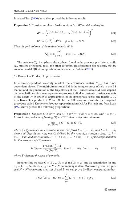
Methodol Comput Appl ProbabImai and Tan (2006) have then proved the following result:Proposition 3 Consider an Asian basket options in a BS model, and def ine( (d (p) μ ∑ ) (p−1= e 1+ k=1 C∗ 1kμ ∑ ))p−1 T,...,eMN+k=1 C∗ MN,k(24)B (p) = ( C Ch) T(d (p) ), p = 1,...,MN. (25)Then the p-th column of the optimal matrix A ∗ isB(p)A∗·p =±‖B (p) ‖p = 1,...,MN. (26)The matrices Cik ∗ , k < p have already been found in the previous p − 1 steps, whileA·p must be orthogonal to all the other columns. This condition can be easily met byan incremental QR decomposition, as described in Sabino (2011).3.4 Kronecker Product ApproximationIn a time-dependent volatility market the covariance matrix MN has timedependentblocks. The multi-dimensional BM is the unique source of risk in the BSmarket and the generation of the trajectories of the 1-dimensional BM does dependon the volatilities. As a consequence we propose to find a constant covariance matrixof the assets H in order to approximate, in an appropriate sense, the matrix MNas a Kronecker product of R and H. In the following we illustrate the proposedprocedure called Kronecker Product Approximation (KPA). Pitsianis and Van Loan(1993) have proved the following proposition:Proposition 4 Suppose G ∈ R m×n and G 1 ∈ R m1×n1 with m = m 1 m 2 and n = n 1 n 2 .Consider the problem of f inding G ∗ 2 ∈ Rm1×n1 that realizes the minimummin ‖ G − G 1 ⊗ G 2 ‖ 2 F , (27)G 2∈R m 1 ×n 1where ‖·‖ 2 F denotes the Frobenius norm. For f ixed h = 1,...,m 2 and l = 1,...,n 2denote R(G) hl the m 1 × n 1 matrix def ined by the rows h, h + m 2 , h + 2m 2 ,...,h +(m 1 − 1)m 2 and the columns l, l + n 2 , l + 2n 2 ,...,l + (n 1 − 1)n 2 of the original matrixG. The elements of G ∗ 2then are(G ∗ 2 ) hl = Tr ( R(G)hl T G )1Tr ( )G 1 G1T h = 1,...,m 2 , l = 1,...,n 2 , (28)where Tr denotes the trace of a matrix.In our setting we have G = MN , G 1 = R and G 2 = H, and we remark that for anyi, j = 1,...,N, R( MN )) ij is a N × N boomerang matrix. Moreover, given two generalN × N boomerang matrices A and B, we can prove by direct computation thatTr(A T B) = Tr(AB) =N∑(2(N − j) + 1) a jj b jj . (29)j=1