Session J.pdf - Clarkson University

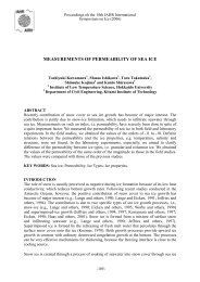
17th International Symposium on IceSaint Petersburg, Russia, 21-25 June 2004International Association of Hydraulic Engineering and ResearchSIDE-VIEWING HIGH-SPEED VIDEOOBSERVATIONS OF ICE CRUSHINGRobert Gagnon 1ABSTRACTRectangular thick sections (1 cm thickness) of lab-grown mono-crystalline ice havebeen confined between two thick Lexan plates and crushed at –10 o C from one edge faceat a rate of 1 cm/s using a stainless steel platen (1 cm thickness) inserted between theplates. The transparent Lexan plates permitted side viewing of the ice behavior duringcrushing and the visual data were recorded using high-speed video. An in-plane fractureoccurs in the ice sample early in the tests and expands from the platen/ice contact areaas load increases. Ice on one side of the in-plane fracture experiences shattering andpulverization while the ice on the other side remains intact but melts at the platen/icecontact where the pressure is high (~ 40 MPa). The continuous production and flow ofliquid at high pressure in a thin layer at the intact ice / platen interface was strikinglyevident and most of the load was supported in this zone. While some spalls did occur atthe intact ice contact zone, cyclic spalling that normally occurs in ice crushingexperiments was suppressed due to the unusual confinement arrangement. The crushingon one side of the in-plane fracture and melting on the other side occurred continuouslyat the nominal platen penetration rate for most of a test, however, when spalls did occurthe relative platen/ice penetration rate was momentarily much higher due to the releaseof elastic energy in the system.INTRODUCTIONSeveral studies of ice crushing behavior have been conducted over of the past fewdecades, driven by the need for understanding and mitigating ice hazards associatedwith offshore oil and gas development and transportation, and shipping in general.Some of the more recent investigations included in situ visual observations. At highstrain rates visual data have been acquired from indentors (Gagnon, 1998; Fransson etal., 1991) and a ship hull (Riska et al., 1990) that incorporated windows for viewing theindented ice surface, and there have also been test apparatus that allowed viewing of theice/indentor interface through the ice samples (Gagnon, 1994a; Gagnon and Mølgaard,1991). The visual data, combined with displacement, load and pressure records, and1 Institute for Ocean Technology, National Research Council of Canada, St. John's, NF, A1B 3T5289

temperature data in a few instances, have lead to significant new insights into the icecrushing process.At low strain rates visually dramatic experiments have been performed by edge-loadingconfined thin sections of polycrystalline ice to demonstrate plastic deformation andrecrystallization (Wilson, 1999). The present study incorporates a similar conceptexcept that the strain rate is much higher, and is in the range associated with icecrushing rather than plastic deformation. The loads are much higher and the apparatus iscorrespondingly stronger. This is the first time that such a technique has been used forice crushing. The visual data from the present side-viewing perspective corroborate withvisual results from other previous experiments and help clarify any ambiguities arisingfrom the earlier viewing perspectives.METHOD AND APPARATUSFigure 1a shows a conceptualschematic of the test method. Theice specimen is a 1 cm thicksection. The sample is confinedbetween two thick plates (12 cm x13 cm 3.8 cm) of transparentacrylic (Lexan). The Lexan platesare mounted in a holder (Figure1b), made from 19 mm thickAluminum plate, that keeps theLexan and ice specimen in place.The Lexan plates are separated bysmall plastic spacers (1 cm thick)between the plates at the sides.The holder provided confinementto the ice sample at the bottomand at the side edges to a height of6 cm from the bottom. Notchesare cut in the upper portion of theside confining plates (above 6 cm)to allow for lateral escape ofcrushed ice during the tests.Aluminum braces, withadjustment bolts, hold the platestogether. The crushing platen wasmade of stainless steel and haddimensions 10 cm x 6 cm x 1 cm.When the ice holder was mountedand carefully aligned in the MTStest frame, the crushing platencould snuggly slide between theLexan plates to make contact withthe exposed edge of the icesample. For the actual testFig. 1. (a) Conceptual schematic of the ice crushing testmethod. (b) Details of the ice holder290

Fig. 2. High-speed video images (with time stamps) from a test using a single crystal ice specimen. Theice slab is in the plane of the image and the view is through a Lexan plate as shown in Figure 1. The ruleat the lower right indicates the scale of the test and the progress of the crushing platen as it insertsbetween the Lexan plates from below at a nominal rate of 1 cm/s. Note that the view is inverted from theschematics shown in Figure 1. The images run downwards from the top left to the bottom right. The testwas conducted at –10 o CWhen the platen makes contact with the ice load begins to accumulate (Figure 4). Thehigh-speed video record shows that one of the ice faces usually looses its adherence tothe Lexan early in the test. As the loss of adherence progresses a fan-shaped fracturesurface appears in the plane of the ice specimen (Figure 2, t=0.096 s) separating the icethat has adhered to the Lexan from the ice that has let go of the Lexan. This in-planefracture continues to extend as the platen moves forward and is about halfway throughthe thickness of the ice slab. Linear out-of-plane cracks also begin to appear in a radialpattern centered at the platen/ice contact zone. The first two of these appear at the sidesof the ice sample within one video frame interval, just as the ice face finishes separatingfrom the Lexan at t=0.098 s (Figure 2, t=0.114 s). These are followed by two other outof-planecracks that appear one after another, 8 and 21 frames later, in the more centralview area with initial lengths of about 3 cm (Figure 2, t=0.158 s). The latter extend fromboth ends to lengthen by 2 or 3 more centimeters over the span of a few imagesimmediately following their appearance. Eventually the in-plane fractures at the sides ofthe image lead to complete separation of pieces from the ice specimen at the peak inload at around t=0.242 s in the test (Figure 2, t=0.476 s).292

Fig. 3. Image from the high-speed video record indicating various aspects of the apparatus and icebehavior. The image is the same as that shown in Figure 2 at t=0.702 sFig. 4. Load record for the test shown in Figures 2 and 3 with markers (open circles) corresponding to the8 video images in Figure 2. Time zero corresponds to the time first contact occurs between the crushingplaten and the ice. Three spall events and a region of the record exhibiting stick-slip are also indicated onthe chart. Spalls 1 and 3 correspond to the images in Figure 2 with time stamps t=0.702 s and t=1.058 srespectivelyApparently the portion of the ice sample on the backside of the large in-plane fracture(relative to the camera), with the face that has lost adherence to the Lexan, is moresusceptible to fracture-generating stresses. This arises because in-plane lateralconfinement is no longer provided by adherence to the Lexan or by attachment to the293

est of the ice, due to the in-plane fracture. Consequently this ice portion shatters and ispulverized as the platen moves ahead. In tests where the intact ice that remains adheredto the Lexan plate faces the camera, the movement of pulverized ice can be seen behindit, such as the test shown in Figures 2 and 3. Alternately, in some tests the pulverizedice is on the side facing the camera, and consequently it blocks the view of the behaviorof the intact ice since it is opaque. Some tests were recorded for both scenarios therebyrevealing the behavior of the pulverized and intact ice in detail. In the video record forthe test under consideration the pulverized ice can be seen flowing away to the left andright from the central region of the ice specimen, where the pressure is higher. Theremaining ice on the front side of the in-plane fracture stays relatively intact however. Itis likely that the pulverized ice provides some degree of confinement that helps theintact ice remain in its undamaged state.While the shattered and pulverized ice is removed from the contact zone by simplyflowing away, a dramatically different mechanism accounts for the removal of intact iceat the ice/platen contact, namely melting. This is evident in the video record that showsa thin layer of liquid extruding from between the platen and ice interface (Figures 2 and3). The liquid aspect of the layer is evident in that it can be seen wetting the pulverizedmaterial adjacent to the sides and behind the intact ice. The liquid can also be seenflowing from between the ice and the platen into the narrow gap between the platen andthe Lexan plate in the plane of the image (Figures 2 and 3), where it then refreezes.Note that during the test setup when the platen is partially inserted between the Lexanplates, that the fit is so snug that there is a little friction between the Lexan and metal.Consequently at the end of a test a roughly semi-circular patch of extremely thin ice,transparent in its upper central area, is visible on the side of the platen where the liquidfroze (Figure 5). The estimated thickness of the thin ice layer is ~ 0.3 mm. This refrozenice causes a portion of the load record to exhibit a regular small-amplitude pattern ofstick-slip (Figures 4 and 6), probably due to the repeated freezing of liquid to the platenand Lexan in the small gap and breakage of the bond as the platen moves.Fig. 5. Crushing platen with a roughly semi-circular patchof extremely thin ice frozen to its side at the leading endfollowing the test shown in Figure 2. The ice layer istransparent in its upper central area and is ~ 0.3 mm thickThe relative movement of the platen against the ice is continuous for most of the recordshown (i.e. at the nominal test rate of 0.010 m/s) except for the instances where spalls294

eak away from the ice/platencontact area that cause abruptsubstantial load drops to occurwhere the penetration rate ismomentarily much higher due to therelease of elastic stress in thesystem. Three such events areevident in the load record (Figure 4)and are shown in an expandedsection in Figure 7. The imagescorresponding to two of the spallevents are shown in Figure 2 att=0.702 s (i.e. same as Figure 3) andFig. 6. Expanded view of the segment of the loadrecord shown in Figure 4 exhibiting small-amplitudestick-slipat t=1.058 s, and occur at the left of the ice/platen contact zone. Spall 2 occurred on theback side of the contact zone, rather than at the left side as in the case of Spalls 1 and 3,and was therefore not as visible. We can estimate the rate of penetration during theload drops induced by the spall events from the load record and the compliance of theice/apparatus system. The compliance of the system was estimated to be around 2x10 -8m/N, from the load and displacement data acquired at the end of a test when the platenwas withdrawn. If we consider the load drop at Spall 3, for example, the load changedfrom 5700 N to 2000 N in 0.2 ms. Hence, using the compliance, we see that the platenmoved against the ice 7.4x10 -5 m in 0.2 ms, that is, at a rate at ~ 0.37 m/s during theload drop (Figure 8).Fig. 7. Expanded view of the segment of the load recordshown in Figure 4 showing three spall events. The highspeedvideo images in Figure 2 associated with two of thespall events are also indicatedWe attach significance tospalling because it is known tobe a major factor in thebehavior of ice impact andindentation. The characteristicsawtooth pattern in load recordsfrom ice indentation tests(Michel and Blanchet, 1983;Evans et al., 1984; Määttänen,1983; Timco and Jordaan,1988; Sohdi and Morris, 1984;Frederking et al., 1990), andshape evolution of the icecontact, stems from spalling atthe high pressure ice/indentorcontact region (Gagnon, 1999). The distinctly different nature of the confinement in thepresent test configuration is probably the reason why cyclic spalling, so characteristic inprevious investigations, did not occur.The melting process has been observed before and explained in detail (Gagnon andMølgaard, 1991; Gagnon 1994a, 1994b; Gagnon and Sinha, 1991). In the region of highpressure contact between the platen and the intact ice a pre-existing thin layer of liquidon the ice surface (Faraday, 1859), or one that is produced by pressure melting, starts toflow because of the extreme pressure. The viscous flow of the liquid generates heat andadditional melting occurs immediately since the liquid layer is in direct contact with ice.295

Fig. 8. Highly expanded view of the segment of the platen/ice relativedisplacement record (left axis) and corresponding segment of the load record(right axis) showing Spall 3. The platen/ice relative displacement was determinedfrom the nominal platen displacement minus the load times the compliance of the systemThe process can happen at relatively slow rates, such as the continuous crushing rateseen in the present load record and also at much faster rates, such as occurs during aload drop where the pressure is momentarily higher. For a given contact area the liquidlayer is thicker at the higher penetration rate (Gagnon, 1994b and 1994b). In either casethe integrity of the ice in the hard spot is preserved. In situ liquid layer thicknessmeasurements have been made in crushing tests on truncated pyramids of ice at asimilar scale to the present tests at a crushing platen displacement rate of 0.5 cm/s, bothat load drops and during the slower rate of penetration on the ascending side of sawteethin the load records. The layer thickness was found to be 2.8 microns for a relativepenetration rate of 0.0014 m/s on the ascending side of sawteeth in the load record, and20.8 microns for the relative penetration rate of 0.26 m/s at load drops (Gagnon, 1994b).In the present tests the relative penetration rate for the continuous crushing portion ofthe test is 0.010 m/s (i.e. the nominal penetration rate) and 0.37 m/s at the load drops.Hence, the high-pressure liquid layer thickness is probably similar in both sets ofexperiments, at least for the load drops.We note that at larger scales, such as the previous Hobson’s Choice Ice Islandindentation tests (Masterson et al., 1993), the relative ice/indentor displacement duringthe ascending portion of the sawteeth in load was very small or none at all, that is, theactuator displacement was mostly taken up elastically in the ice/apparatus system(Gagnon, 1998). The majority of the actual ice/indentor relative displacement occurredat the load drops, caused by spall events, at a high displacement rate. These, and othercharacteristics, have been discussed in detail (Gagnon, 1998).We can get a rough estimate of the pressure existing at the ice/platen interface on theintact ice from the measured load and by estimating the area of contact, assuming thepulverized ice that flows away to the sides will be supporting much less pressure. Thelength of the intact ice contact is clearly evident from the video record. Its thickness isestimated to be half the thickness of the ice slab (5 mm). Assuming the load is appliedto this estimated contact area we obtain a pressure of about 40 MPa. This is quiteconsistent with in situ pressure measurements obtained from the earlier experiments296

(Gagnon, 1999). To further support the assumption that the intact ice supports themajority of the load we can compare the actual measured extent of the load drops, onthe charts (Figures 7 and points a and b in Figure 8), with the change in contact area ofintact ice due to the spalls from the video record. We see that the load drop for Spall 1amounts to a reduction of contact area of about 25% (Figure 2, t=0.702 s and Figure 3)that matches well with the drop in actual load, about 25%. Similarly for Spall 3 inFigure 2 at t=1.058 s, the change in area is about 66% and the load drop iscorrespondingly 65%. Note that the measurement of the actual drop in load from theload record, that is, the precise location of points a and b in Figure 8, takes into accountthe resonance in the system that occurs immediately after the spall for a brief period.In summary we note the following similarities between previous tests and the presentones. 1. Regions of intact ice exist where the pressure is high at the ice/platen interface.2. Melting, and flow of the melt in a thin layer at the high-pressure contact interfaceoccurs. 3. Rapid relative displacement of the platen/ice occurs during load drops. This iscaused by spalling at the intact ice/platen interface. Consequently much higher rates ofmelting and liquid flow occur at the load drops than at other times during the crushingtests.The primary difference observed between previous experiments and the present testresults was that the sawtooth load pattern, due to cyclic spall events, was not evident inthese tests, although spalls did occur from time to time. This is likely the result of theconfinement differences. Since spalling was not prevalent in the present tests thepenetration was continuous for the most part, i.e. at the nominal rate of platenpenetration, whereas when cyclic spalling occurs, as in previous tests, the actualpenetration rate on the ascending portions of the sawtooth load is lower than thenominal rate, or negligible, due to compliance of the ice/indentor system.The mechanism responsible for the majority of the energy dissipation, however, is thesame in the present and previous studies, namely melting and viscous flow of melt(Gagnon, 1999).CONCLUSIONSA new type of ice crushing experiment has been conducted that enables a unique sideviewingperspective of the ice behavior.The important phenomena of melting, due to viscous flow of a thin layer of highpressureliquid at the ice/structure interface, and spalling at the ice contact zone havebeen observed in unprecedented detail. The frequency of spall events in the present testsis much less than is normally observed in ice crushing, probably due to the verydifferent confinement aspects of the test setup.As in previous crushing experiments, high-speed video has proven to be a very usefuldata acquisition system and an invaluable tool for interpretation of the results.It would be very instructive to conduct similar tests at larger scales.ACKNOWLEDGEMENTSThe author would like to thank the Program of Energy Research and Development(PERD) for their financial support of this research.297

REFERENCESEvans, A.G., Palmer, A.C., Goodman, D.J., Ashby, M.F., Hutchison, J.W., Ponter, A.R.S. and Williams,G.J. 1984. Indentation spalling of edge-loaded ice sheets. IAHR Ice Symposium, Hamburg, 113-121.Faraday, M. 1859. On regelation, and on the conservation of force. Phil. Mag. 17, 162-169.Fransson, L., Olofsson, T. and Sandkvist, J. 1991. Observations of the Failure Process in Ice BlocksCrushed by a Flat Indentor. Proceedings of the 11th International Conference on Port and OceanEngineering Under Arctic Conditions, St. John's, Canada, Vol. 1, 501-514.Frederking, R., Jordaan, I.J. and McCallum, J.S. 1990. Field Tests of Ice Indentation at Medium Scale,Hobson's Choice Ice Island, 1989. Proceedings of the 10th International Symposium on Ice (IAHR 90),Espoo, Finland, Vol. 2, 931-944.Gagnon, R.E. 1994a. Generation of Melt During Crushing Experiments on Freshwater Ice. Cold RegionsScience and Technology, Vol. 22, No. 4, 385-398.Gagnon, R.E. 1994b. Melt Layer Thickness Measurements During Crushing Experiments on FreshwaterIce. Journal of Glaciology, 1994, Vol. 40, No. 134, 119-124.Gagnon, R.E. 1998. Analysis of Visual Data from Medium Scale Indentation Experiments at Hobson’sChoice Ice Island. Cold Regions Science and Technology, Vol. 28, 45-58.Gagnon, R.E. 1999. Consistent Observations of Ice Crushing in Laboratory Tests and Field ExperimentsCovering Three Orders of Magnitude in Scale. Proceedings of the 15th International Conference on Portand Ocean Engineering under Arctic Conditions, POAC-99, Helsinki, Finland, Vol. 2, 858-869.Gagnon, R.E. and Mølgaard, J. 1991. Evidence for pressure melting and heat generation by viscous flowof liquid in indentation and impact experiments on ice. Proceedings of the IGS Symposium on Ice-OceanDynamics and Mechanics, 1990, New Hampshire, Ann. of Glaciol., 15: 254-260.Gagnon, R.E. and Sinha, N.K. 1991. Energy Dissipation Through Melting in Large Scale IndentationExperiments on Multi-Year Sea Ice. Proc. of the 10th International Conference on Offshore Mechanicsand Arctic Engineering, Stavanger, Vol. IV, Arctic/Polar Technology, 157-161.Määttänen, M. 1983. Dynamic ice-structure interaction during continuous crushing. CRREL Rep. 83-85.Masterson, D.M., Frederking, R.M.W., Jordaan, I.J. and Spencer, P.A. 1993. Description of multi-year iceindentation tests at Hobson’s Choice Ice Island - 1990. Proceedings of the 12th International Conferenceon Offshore Mechanics and Arctic Engineering, Vol. 4, 145-155.Michel, B. and Blanchet, D. 1983. Indentation of an S2 floating ice sheet in the brittle range. Ann.Glaciol., 4: 180-187.Riska, K., Rantala, H. and Joensuu, A. 1990. Full scale observations of ship-ice contact.Laboratory of Naval Architecture and Marine Engineering, Helsinki University of Technology, ReportM-97.Sodhi, D.S. and Morris, C.E. 1984. Ice forces on rigid, vertical, cylindrical structures. CRREL Rep. 84-33.Timco, G.W. and Jordaan, I.J. 1988. Time series variations in ice crushing. Proceedings of the 9thInternational Conference on Port and Ocean Engineering Under Arctic Conditions, Fairbanks, Alaska,13-20.Wilson, C.J. 1999. Downloadable movie from the website of the School of Earth Sciences - TheUniversity of Melbourne - Australia. Copyright Notice - The University of Melbourne, 1994 - (2000).http://web.earthsci.unimelb.edu.au/wilson/ice1/index.html298

17th International Symposium on IceSaint Petersburg, Russia, 21-25 June 2004International Association of Hydraulic Engineering and ResearchIN-SITU FRACTURE OF FIRST-YEAR SEA ICEIN McMURDO SOUNDJohn P. Dempsey 1 , Zonglei Mu 1 and David M. Cole 2ABSTRACTThe breakup of sea ice in McMurdo Sound has been studied during two field trips in thefall of 2000 and 2001 via in-situ cyclic loading and fracture experiments. In Cole et al.(2002), the motivation, test site, experimental setup, cyclic response and associatedacoustic emission for the 5 ×5 m 2 test specimen A2-SP2 were presented. In Dempsey etal. (2003), the fictitious crack model, which makes uses of the stress-separation curve,was used to incorporate a process zone into the fracture analysis. The cracking behaviorobserved and measured on A2-SP2, during both the cyclic loading and the displacementcontrolled ramp to tensile fracture was examined. Preliminary estimates of the fractureenergy were provided. In this paper, stress-separation curves for the A2-SP2 experimentare constructed such that the response computed using the fictitious crack modelmatches the experimental results. A bilinear stress-separation curve is back-calculatedfor first-year Antarctic sea ice. The changing shape of the stress separation curve duringcrack growth is studied. It is hypothesized that this change is reflective of a multiplecrack path competitive process.ACRONYMSCMODCODCTODFCMFPZNCTODcrack-mouth-opening-displacementintermediate-crack-opening-displacementcrack-tip-opening-displacementfictitious crack modelfracture process zonenear-crack-tip-opening-displacementINTRODUCTIONThe breakup of floating first-year Antarctic sea ice is investigated in this paper, with thegoal of developing improved, physically based models of this important process. Twofield trips have been conducted in McMurdo Sound, Antarctica in support of this objective.1 Clarkson University, Potsdam, New York, USA2 US Army ERDC-CRREL, Hanover, New Hampshire, USA299

The in-situ experiments conducted during the October-November 2001 field tripwere located at S 77° 35.033′ E 166° 06.005′, approximately 3 km offshore fromCape Barne on Ross Island. Cole et al. (2002) described the test site, experimentsetup and methods used in the in-situ experiments on the through-thickness specimenA2-SP2 of first-year sea ice measuring 5 × 5 m 2 , and presented results for thecyclic loading response, acoustic emission activity and physical properties. Oncethe constitutive testing was completed, the specimen was loaded to failure in eitherload or displacement control to obtain its fracture behavior. Dempsey et al. (2003)then concentrated on the fracture behavior measured and observed in the samespecimen A2-SP2. Several separate tests of A2-SP2 were examined and a preliminaryestimate of the critical crack-tip-opening-displacement was found. In order tomeaningfully interpret the fracture results, the fictitious crack model (FCM) wasadopted to describe the fracture of A2-SP2. Hillerborg et al. (1976) first proposedthis cohesive zone model for the fracture of concrete. It is a nonlinear cohesivezone model that includes the tension softening process zone through a fictitiouscrack (without complete separation of the crack faces) ahead of the traction-freecrack. In the fictitious crack it is possible to distinguish two zones: a real crackwhere there are no tractions, and a damaged zone, denoted as the fracture processzone (FPZ), in which stresses are still transferred. The response of material pointslying in the fracture process zone is governed by the stress-separation curve, whichrelates the opening of the crack faces w to the cohesive stress σ fpz . As such, thestress-separation curve σ fpz (w) and the area under this curve G c are the fundamentalproperties defining the fracture. In the present paper, an effort is made to deducethe stress-separation curve by matching the response of the fractured specimenwith that from the fictitious crack model such that the distribution of cohesivestress within the process zone for any geometry and crack size is known.THE FRACTURE OF A2-SP2The in-situ fracture test discussed in this paper is the 5 m square plate of sea icelabeled A2-SP2 (Figure 1). The test configuration is shown in Figure 1a. All dimensionsare in cm. The LVDT ranges (± ranges) are in microns. Both a ‘coarserange’ ( c ) and a ‘fine range’ ( f ) gage were used to record the crack-mouth-openingdisplacement(CMOD), intermediate-crack-opening-displacement (COD), andnear-crack-tip-opening-displacement (NCTOD). The notation NCTOD ± indicatesthat the LVDT concerned was placed 10 cm ahead of ( + ) or before ( − ) the crack tip.So-called ‘fictitious’ gages (F1, F2 and F3) were also placed ahead of the crack tipto identify the crack-opening-displacement when the crack advanced.300

Fig. 1. a) The test configuration for A2-SP2; b) closer look at LVDT and AE sensor locations ahead of thecrack tip; c) Side view of the pre-sawn crack, flatjack placement, and schematic of the crack frontExperimental results and discussionAs described in Dempsey et al. (2003), even though many of tests of A2-SP2 were targetingthe cyclic behavior of the first-year sea ice, the cyclic loading also induced crackingin the vicinity of the traction-free crack tip. As A2-SP2 was subjected to more andmore cycles, it was possible to follow the growth of the FPZ. The fracture behavior ofTests #4, #6 and #7 were thoroughly examined by Dempsey et al. (2003).Fig. 2. Test #15: a) NCTOD ± , F1, F2 and F3 vs time; b) Load vs NCTOD ± , F1, F2 and F3301

In Test #15, the objective was to stably fracture the 5m square test piece. Therefore, indisplacement control, the CMOD was subjected to a sine-curve-shaped ramp versustime such that tensile failure would occur in less than 50 s (the peak load of 76.2 kN occurredat 36.8 s). The load and crack-opening-displacement behavior at some of thegages are portrayed in Figure 2. Note that the fracture behavior of this first-year sea icein McMurdo Sound was studied by measuring the crack-opening-displacements at thesurface only. It is an especially difficult matter to determine what the critical separation(w c ) for this ice is. In other words, what is the critical CTOD for growth of the tractionfreecrack to initiate? When the crack did propagate, it veered to the left slightly, justpassing to the left of the F3 gage (see the crack path in Figure 3). In Figure 2a, note thatthe F3 versus time plot shows a sudden relaxation; this occurs at t= 35.7 s, at an openingload of 72 kN, and at a gage separation of 77 µm. The interpretation is that a FPZ hadbeen getting established straight ahead of the traction-free crack path, in addition to aFPZ on the final crack path, until suddenly crack growth along the final path was foundto be easier (no doubt due to a mild alignment of the ice fabric at the test site). For thisreason, one can hypothesize that w c > 77 µm. Until one sees crack-openingdisplacementsof this magnitude in the FPZ, growth of the traction-free crack is notlikely.Modeling the experimental responseFig. 3. Crack path of A2-SP2 after testIn the fictitious crack model, the stress separation and specimen material behavior canbe modeled as viscoelastic. For the present set of experiments, the stress-separationcurve as well as the viscoelastic characterization of the sea ice is not known. Moreover,it does not seem possible to conduct direct tension in-situ experiments in the field to experimentallyobtain these material parameters. However, this information can be backcalculatedsuch that predicted results match the experimental results. Dempsey andMulmule (1998) developed a viscoelastic fictitious crack model for the fracture of sea302

ice. The same procedure is used here to carry out the match between the model and experiment.Figure 4 shows a representative set of results for A2-SP2. To ensure the accuracyof the iteration procedure, the loading must be applied at the same rate as duringthe experiment. Figure 4a shows the experimentally applied load and the load applied tothe model. Due to unexpected indentation of the flatjack, the initial loading actually beganaround 20kN. Figure 4b shows experimental crack opening displacements comparedto the matched response of the model: at about 36s, the crack-tip-openingdisplacement(CTOD) may reach the critical-crack-tip-opening-displacement before instabilityoccurs because of stable crack growth.Fig. 4. Comparison of the experimental and matched (a) flatjack pressure vs time;(b) crack-opening-displacement vs timeMany different shapes of stress-separation curves have been used for different materials.Figure 5a shows various shapes of stress-separation curves that have been proposed.Shape ABC is the Dugdale distribution with a cutoff (see page 161 in Bažant andPlanas, 1998). Shape AC is linear softening (a common approximation). Shape AEC isthe concave bilinear shape that is found for concrete (Guinea et al. 1994). For the firstyearsea ice discussed in this paper, Figure 5b shows the back-calculated stressseparationcurve for A2-SP2 that is applicable prior to growth of the traction-free crack.Note that a convex bilinear shape is needed, as was also found by Mulmule andDempsey (1999) for colder Arctic ice. The creep compliance expression used to matchthe experimental and model results for A2-SP2 is J=1/E+Ct 1/2 , where E=3.1 GPa andC=3.5×10 -11 m 2 /Ns 1/2 . The critical CTOD obtained from the stress-separation curve is80 µm; this also matched the preliminary estimate discussed above. The critical CTODfor the Antarctic A2-SP2 test is larger than that of Arctic ice, while the tensile strengthis smaller. These changes may well be caused by the warm weather under which theA2-SP2 specimen exhibited more ductile behavior. Under such circumstances, the effectivelength of the crack may increase. The fictitious crack model theory explains thelarger critical CTOD. The critical fracture energy to initiate stable propagation of thetraction-free crack (13 J/m 2 ) in A2-SP2 is slightly smaller than its colder Arctic counterpart(15 J/m 2 ). The fully-grown size of the process zone in A2-SP2 is about 190 mm.303

Fig. 5. (a) Various stress-separation curve shapes applicable for different materials;(b) Back-calculated stress-separation curve for A2-SP2Fig. 6. Back-calculated stress-separation curves for A2-SP2 with growth of traction-free crackIn order to investigate how crack growth affects the fracture description, a number ofstress curves were constructed, each associated with a specific amount of growth of thetraction-free crack. These curves are shown in Figure 6. The behavior is indicative of anincrease in fracture energy with crack propagation (Figure 7a). Post-test observationsshowed that the propagating crack seeks out planes of weakness within the microstructure,either following favorably oriented plate boundaries or larger-scaled brine drainagefeatures. Branches were observed to run from the main crack and terminate at distancesof approximately 0.1 m from the crack face. These branches were frequently associatedwith brine drainage features. Occasionally, a crack branch would rejoin the main crackand thereby break sections of material free of the crack face. These post-test observationsindicated that observed changes in the stress-separation behavior with crackgrowth may be reflective of a multiple crack path competitive process. With increasing304

crack growth, the tensile strength and critical CTOD is increasing. The fictitious crackmodel predicts a decreasing size of the process zone with crack growth (Figure 7b).CONCLUSIONSFig. 7. (a) Fracture energy vs stable crack growth for A2-SP2;(b) Decreasing fracture process zone length with crack growthThe experimental measurements and numerical calculations presented in the foregoinglead to the following observations:1. Hillerborg’s fictitious crack model can be applied to the fracture of floating firstyearsea ice in Antarctica. The stress-separation curve for first-year Antarctic sea ice isconvex and bilinear.2. The length of the fracture process zone decreases with crack growth. A change inthe stress-separation behavior with crack growth is reflective of a multiple crack pathcompetitive process.SIGNIFICANCEThe significance of the above findings rests with the resulting ability to predict the formationand behavior of a tensile crack in first-year sea ice. The fictitious crack modelcan describe the formation of a crack in an unnotched configuration, the growth of thiscrack to any extent, and the influence of specimen size as well as geometry. That is,with the stress-separation curve at hand, and given a chosen test geometry, the specimensize effects to be expected can be accurately predicted (Mulmule and Dempsey, 1999).ACKNOWLEDGEMENTSThe support of NSF's Antarctic Sciences Ocean and Climate Program, grants OPP-9873629 and OPP-9909100, and Dr. Bernhard Lettau, the program manager, are gratefullyacknowledged.REFERENCESBažant, Z.P. and Planas, J. Fracture and Size Effect in Concrete and Other Quasibrittle Materials. CRCPress (1998).Cole, D.M., Dempsey, J.P., Kjestveit, G., Shapiro, S., Shapiro, L.H. and Morley, G.M. The cyclic andfracture response of sea ice in McMurdo Sound: observations from in-situ experiments. Part I. In 16thIAHR International Symposium on Ice, Vol. 1, University of Otago, Dunedin, New Zealand (2002) 474-481.305

Dempsey, J.P., Cole, D.M., Shapiro, S., Kjestveit, G., Shapiro, L.H. and Morley, G.M. The cyclic andfracture response of sea ice in McMurdo Sound. Part II. In Proceedings of the 17th International Conferenceon Port and Ocean Engineering under Arctic Conditions, Vol. 1, Trondheim, Norway (2003) 51-60.Guinea, G.V., Planas, J. and Elices, M. A general bilinear fit for the softening curve of concrete. Materialsand Structures 27: 99-105 (1994).Hillerborg, A., Modéer, M., and Petersson, P.E. Analysis of crack information and crack growth in concreteby means of fracture mechanics and finite elements. Cement and Concrete Research 6: 773-781(1976).Mulmule, S.V. and Dempsey, J.P. A viscoelastic fictitious crack model for the fracture of sea ice. Mechanicsof Time-Dependent Materials 1: 331-356 (1998).Mulmule, S.V. and Dempsey, J.P. Scale effects on sea ice fracture. Mechanics of Cohesive-FrictionalMaterials 4: 505-524 (1999).306

17th International Symposium on IceSaint Petersburg, Russia, 21-25 June 2004International Association of Hydraulic Engineering and ResearchICE PRESSURE VARIATIONS DURING INDENTATIONR. Frederking 1ABSTRACTThe Japan Ocean Industry Association made available to the IAHR Ice Crushing WorkingGroup one data file from a field test conducted February 4, 1999. An indenter 1.5 mwide by 0.5 m high, penetrated a sea ice sheet 168 mm thick at a rate of 3 mm/s for atotal penetration of 1000 mm. The entire indenter face was covered with “tactile” sensorelements, each nominally 10 mm by 10 mm. Spatial distributions of local pressure wererecorded throughout the test as well as the total load measured with a load cell. Detailedanalysis of the results showed that the load cell and tactile sensors gave comparable results.The tactile sensors showed a “line-like” load distribution with only about 10 % ofthe ice edge in load-bearing contact. “Hot-spots” of high local pressure persisted forsurprisingly long periods, up to 10 s. Local pressure variations tended to be synchronous,that is largely increasing and decreasing with global load.INTRODUCTIONThe nature of local ice pressure distributions during indentation has been a subject ofinterest for some time in ice mechanics. It is an important factor in developing an understandingof the ice failure process since this understanding provide one of the means ofscaling-up small-scale laboratory and field measurements to scales needed for design ofoffshore structures and ship hull structures. Obtaining good measurement data on pressurewithin the contact area was always a problem. If the sensor area was large, thepressure was averaged over too large an area; if the sensor area was small, there wereusually insufficient sensors to determine the distribution of pressures. Load cells tomeasure average pressures over areas as small as 10 mm dia. were employed in laboratoryand field measurements (Masterson et al, 1999, Sayed et al, 1992). Local pressuresas high as 80 MPa were measured on a 10 mm diameter sensor in indentation of multiyearice (Frederking et all, 1990). Early work in Finland (Joensuu, 1988) initiated theuse of PVDF sensors to almost completely cover the measurement area. Later this typeof instrumentation was deployed for field indentation teats on multi-year (Masterson etal 1993) and pressures as high as 50 MPa were measured.More recently the Japan Ocean Industries Association (JOIA) sponsored a project onMedium Scale Field Indentation Tests (MSFIT) of ice sheets which ranged in thickness1 Canadian Hydraulics Centre, National Research Council Canada, Ottawa, Ont. K1A 0R6 Canada307

from 120 mm to 270 mm. During the JOIA project detailed measurements of total load,loads on segments and local pressure distributions were made. The objective of the projectwas to obtain high quality data that could be used to improve the prediction of iceloads on structures. A general description of the test equipment and testing procedurecan be found in Nakazawa et al (1999). To encourage broader understanding of the results,JOIA made available one data file to the IAHR Ice Crushing Working Group foranalysis. These are the data examined in this paper. Spatial and temporal distributions ofpressure will be examined, both on the basis of average distributions, shape of contours,simultaneity and variations during load cycles. Implications for describing ice crushingprocesses will be discussed.DESCRIPTION OF TESTThe MSFIT program was conducted over 5 winters in the late 1990s at Notoro fishingharbour on the North coast of Hokkaido Island, Japan. The data file, from a test conductedFebruary 4, 1999 was for the following conditions:Indenter width = 1500 mmIndenter height = 500 mmIce thickness = 168 mmIndenter speed = 3 mm/sTotal stroke = 1000 mmIce strength = 2.46 MPa.The total load exerted by the actuator was measured with a load cell and recorded at arate of 50 readings a second. The entire indenter face was covered with “tactile” sensorelements, each nominally 10 mm by 10 mm, for a total of 6336 sensor elements (144elements across and 44 elements vertically). The ice was not thick enough to ensurecontact with all the sensor elements, but about 2500 elements contacted the ice edge.Data from the tactile film was recorded at a rate of one “frame” every 0.2667 s (3.7 Hz).A “frame” comprised a 144 by 44 matrix of “pressure” readings. Each element of thetactile film gave an integer reading between 0 and 255. The manufacturer of the filmprovided the following guide to convert output reading to pressurereading pressure (MPa)0 055 0.68255 6.86with a linear relation. It was also stated that the error in any reading on the tactile filmcould be up to ± 10%, so it was recommended that pressure data be treated as relative.The load record from the load cell is presented in Figure 1. It can be seen that there israpid build-up of load to a high peak with the flat indenter making perfect contact withthe flat sawed edge of the ice sheet. Using the indenter width of 1500 mm and the 168mm ice thickness, the average pressure to initially fail the ice sheet was almost 3 MPa.Subsequently the average pressure was never greater than 0.5 MPa. The test was run ata constant actuator rate of 3 mm/s for 300 s (50 s is equivalent to 150 mm indentation).Immediately after the initial failure, fluctuations in the load were small. For the interval40 to 70 seconds (Figure 2), the fluctuations were still small with a pattern of a generalrise followed by a rapid drop off with an irregular period of 5 to 10 seconds. At around80 seconds (Figure 3) the fluctuations settled into a more regular pattern with a frequencyof about 1.2 Hz and the peak-to-trough ratio of the amplitude about 2. It can be308

seen that the nature of the load fluctuations changes significantly between the two timeintervals (Figures 2 and 3). The pattern demonstrated in Figure 3 tended to persist forthe remainder of the test. Also shown in Figure 2 and 3 is a total load determined fromthe tactile film records. This will be discussed further.LOAD (kN)8006004002003 mm/s1500 mm wide flat indenter168 mm ice thiickness3AVER AG E PRESSURE (M Pa)AVERAGE PRESSURE (MPa)21000 50 100 150 200 250 300TIME (sec)Fig. 1. Load – time record for test on February 2, 1999200150Load celltactile filmLOAD (kN)100500PEAKTROUGH40 45 50 55 60 65 70TIME (sec)Fig. 2. Load – time record expanded for interval 40 to 70 secondsThe tactile film data were used to determine total load using a rather simple method ofassigning a load of 1 N per reading unit; that is, a reading of 10 is equivalent to 10 N.Thus the total load in kN is just the sum of all tactile cell readings divided by 1000. Thisis the method used to obtain the tactile film loads presented in Figures 2 and 3. The recordingfrequency of the tactile film determined loads is much less than the load cell,approximately 4 Hz versus 50 Hz, but the tactile film traces follow the trend of the load309

cell determined loads quite closely. Different recording systems were used so the loaddrop from the initial failure was used as an initial synchronizing point, but no furthersynchronization was used throughout. This basis to calculate total load implies a pressureof 2.55 MPa for a reading of 255, rather than the value of 6.8 MPa given by themanufacturer, and again emphasizes that pressures be treated a relative, not absolute.LOAD (kN)20015010050Load celltactile film070 75 80 85 90 95 100TIME (sec)Fig. 3. Load – time record expanded for interval 70 to 100 secondsDISTRIBUTIONS OF PRESSUREThe nature of ice pressure distributions at different points in the loading process will beexamined next. At the 65 second mark (see Figure 2) two successive tactile film recordswere selected, one at 65.26 s just before failure, “peak”, followed by one at 65.53 s, justafter failure, “trough”. The nature of, and change between the two will be discussed.The total loads at the two times, as estimated from the tactile film, are 85 kN and 53 kN,respectively, about a 40% decrease. Contour plots of the two times for the entire iceedge in contact with the indenter (168 mm by 1500 mm) are presented in Figure 4. Thevalues plotted are the pressure numbers, within the range 0 to 255, from the tactile filmrecord (note; all subsequent plots and discussion treat pressure as unitless). What can beseen firstly is that the area subjected to ice pressure is greater at the peak than the trough(290 elements at the peak and 255 at the trough), a 10% decrease so this alone does notaccount for the magnitude of the decrease. Note that the total possible number of cells incontact with the ice edge is 2448, so only about 10% are actually loaded. The number ofcells subjected to ice pressures greater than 10, 25, 50 and 75 was determined and thegreatest difference between the two cases was for pressures greater than 50 (see Table1). At the peak there were 57 cells above that level, but only 15 at the trough. A numberof vertical profiles of pressure were also examined, and they showed that generally thedistribution was peakier at peak load than in the trough. Two immediately adjacent verticalpressure profiles at peak and trough are shown in Figure 5 to illustrate this point.310

1(a)6111621260-25 25-50 50-75 75-100 100-125 125-1503136414651566166717681HORIZONTAL869196101106111116121126131136PEAK1411591317VERTICAL(b)TROUGH17131925313743495561677379859197103109115121HORIZONTALFig. 4. Contour plots of pressure at 65 s; (a) peak, (b) trough1271331391591317VERTICALTable 1. Number of tactile elements loaded at 65 sPressure range Peak Trough> 0 291 2550 to 10 69 8510 to 25 97 9525 to 50 68 6050 to 75 37 12>75 20 3HORIZONTAL POSITION 117PRESSURE0 20 40 60 80DEPTH (mm)1030PEAKTROUGH507090110130150170DEPTH (mm)HORIZONTAL POSITION 118PRESSURE0 20 40 60 8010PEAK30TROUGH507090110130150170Fig. 5. Vertical pressure distributions at 65 s311

Figure 6 presents the horizontal distribution of pressure summed on a vertical axis forthe whole width of the indenter. It can be seen that for the most part the two pressuredistributions are of similar magnitude for both the peak and trough. It is only for horizontalpositions 100 to 140 that the total peak pressures are greater.250TOTAL PRESSURE20015010050PEAKTROUGH00 24 48 72 96 120 144HORIZONTAL POSITIONFig. 6. Total pressure along a vertical line of elements at 65 sAs was shown in Figure 4, the line-like load distribution was generally not continuousacross the entire width of the indenter, even at the time of peak load. What was also observedat some times was a double peak in the vertical distribution of pressure. Figure 7plots six immediately adjacent vertical pressure profiles, covering a width of 60 mm,and all show similar double peaks. This double peak is likely a measurable representationof horizontal cleavage cracks that have been observed in indentation tests. A contourplot of the area from which the vertical profiles of Figure 7 were extracted (Figure8) more clearly illustrates two line-like loaded areas. Figure 8 also illustrates that thehigh pressure between horizontal positions 100 and 120 has persisted for 5 seconds. Infact, this high pressure area or “hot spot” persists to a greater or lesser extent for the entiretest run.1030PRESSURE0 20 40 60 80 100 12070.1 s50DEPTH (mm)7090110130150170Fig. 7. Vertical pressure distributions at 70.1 s312

1080-10060-8040-6020-400-2060110160DEPTH (mm)101 104 107 110 113 116 119HORIZONTAL POSITIONFig. 8. Contour plot of pressure distribution at 70.1 sTo illustrate further pressure distributions and persistence of “hot spots” a contour plotat time 86.1 s is presented in Figure 9. Here there are three horizontal line-like loads andthe high pressure areas are still evident in the horizontal position area 100 to 140.104070100130160100103106109112115118121124127130133DEPTH (mm)136139142HORIZONTAL0-10 10-20 20-30 30-40 40-5050-60 60-70 70-80 80-90 90-10086.1 sFig. 9. Contour plot of pressure at time 86.1 s, a time of peak loadSUMMARYAn indentation test at 3 mm/s on 168 mm thick sea ice provided detailed information onpressure distributions through use of “tactile” file sensor elements covering the entireface of the 1500 mm wide indenter. Summing the tactile sensor data gave total loadssimilar to those from a load cell that measured total load. The tactile sensors showed a“line-like” load distribution with only about 10 % of the ice edge experiencing any localpressure at all. Local pressure distribution before and after failure indicated that the contactarea was essentially the same in both cases, but that there was a larger area of highpressure just before failure. The line-like load distribution was observed to divide into313

two or more horizontal parallel lines, suggesting cleave crack formation. “Hot-spots” ofhigh local pressure persisted for surprisingly long periods, say up to 10 s, and tended tobe in the middle portion of the ice edge.ACKNOWELDGEMENTSThe author would like to acknowledge the financial support for this work from the Programof Energy Research and Development (PERD) through the ice-structure interactionactivity, and the Japan Ocean Industry Association for making these data available.REFERENCESFrederking, R., Jordaan, I.J. and McCallum, J.S. 1990. Field Tests of Ice Indentation atMedium Scale, Hobson's Choice Ice Island, 1989. Proc. IAHR 10th International Symposiumon Ice. August 20-23, 1990. Espoo, Finland, Vol. 2. pp. 931-944.Joensuu, A. 1988. Ice Pressure Measurements using PCDF Film. Proceedings 7th InternationalConference on Offshore Mechanics and Arctic Engineering (OMAE 1988),Houston, February 7-12, 1988, Vol. IV, p. 153-158.Masterson, D.M., Spencer, P.A., Nevel, D.E. and Nordgren, R.P. 1999. Velocity EffectsFrom Multi-Year Ice Tests. 18th International Conference on Offshore Mechanics andArctic Engineering, OMAE99, St. John's Newfoundland.Masterson, D.M., Frederking, R.M.W., Jordaan, Ian J., and Spencer, Paul A. 1993. Descriptionof Multi-Year Ice Indentation Tests at Hobson's Choice Ice Island - 1990. Proceedingof the 12th International Conference on Offshore Mechanics and Arctic Engineering,(OMAE 1993), June 20-24, 1993, Vol. IV, pp 145-155, Glasgow, Scotland.Nakazawa, N., Akagawa, S., Kawamura, M., Sakai, M., Matsushita, H., Terashima, T.,Takeuchi, T., Saeki, H. and Hirayama, H. 1999. Medium Scale Field Ice IndentationTest (MSFIT) – Results of 1998 Winter Tests. Proceedings 9 th (1999) International Offshoreand Polar Engineering Conference, May 30 – June 4, 1999, Vol. II, pp 498-504Brest, France.Sayed, M. and Frederking R. 1992. Two-dimensional Extrusion of crushed ice. Part 1:Experimental. Cold Regions Science and Technology, Vol. 21, pp 25-36.314

17th International Symposium on IceSaint Petersburg, Russia, 21-25 June 2004International Association of Hydraulic Engineering and ResearchPOST-TERMINAL COMPRESSIVE DEFORMATION OF ICE:FRICTION ALONG COULOMBIC SHEAR FAULTSA.Fortt 1 and E.M. Schulson 1ABSTRACTCoulombic shear faults characterize terminal failure when polycrystalline ice Ih is rapidlyloaded under a moderate degree of confinement. Post-terminal deformation occursthrough frictional sliding along the shear fault. To examine this latter stage of deformation,experiments were performed on freshwater S2 ice at –10 o C. The ice was proportionallyloaded biaxially across the column-shaped grains along a variety of allcompressiveloading paths at four sliding velocities (8 × 10 -1 , 8 × 10 -2 , 8 × 10 -3 and 8 ×10 -4 mm/s.). At each velocity Coulomb’s law describes the relationship between theshear strength of the fault and the normal stress across it, both at the onset of sliding andonce sliding has progressed a few millimeters. The friction coefficient decreases withincreasing velocity in a manner similar to that seen by Kennedy et al. (2000) in ice-oniceexperiments, but is higher by about a factor of two to four, depending upon the slidingvelocity. The difference is attributed to surface roughness.INTRODUCTIONThe compressive behavior of S2 ice has been extensively studied (for review, seeSchulson, 2001) in response to the need to predict forces on engineered offshore structuresfrom ice sheets pushing on them. Forces exerted by, and thus on the sheets, aredependent on environmental conditions, such as the wind/ocean currents. The rate atwhich these forces develop, in turn, dictates whether the ice deforms in either a brittle ora ductile manner. Coulombic shear faults denote brittle behavior, which occurs when theice deforms at a rate greater than a critical value (Schulson, 2001) and results in fracturedice. Under compressive loading the fragments slide past one another against frictionalresistance. Understanding that resistance is important to predicting the movementof these fragments. The purpose of this paper, therefore, is to describe the results of experimentsaimed at evaluating the frictional resistance to sliding, following terminalfailure via Coulombic faulting.EXPERIMENTAL PROCEDURESExperiments were performed on fresh-water S2 columnar ice, grown in the laboratory,using established procedures described by Smith and Schulson (1993). In S2 ice thecaxes of the hexagonal unit cell are randomly oriented in a plane perpendicular to the1 Thayer School of Engineering, Dartmouth College, Hanover, NH315

long axes of the columns (Michel, 1978). The microstructure of the ice is shown inFig. 1, along with the reference co-ordinate system. Plate-shaped specimens were cutfrom a parent sheet into prisms with dimensions along X 1 and X 2 of 160 mm and ofthickness through X 3 of 50 mm, with all surfaces parallel to a tolerance of ± 0.1 mm.All experiments were conducted inside a cold room at –10 ± 0.2°C using a multi-axialtesting machine (MATS), in two stages. The first stage consisted of creating a shearfault within the specimen, Fig. 2a, 2b, and the second stage, of sliding along the fault,Fig 2c, 2d.(a)Fig. 1. (a) S2 Ice. (b) The crystallographic orientation of C-axes with respect to the horizontal planeof the parent puck, plotted on a Wulff net(b)(a) (b) (c) (d)Fig. 2. (a) Schematic representation of faulting stage. (b) Illustration showing faulted specimen afterre-machining specimen end parts A & B (shown in (a)). (c) Schematic representation of moment-freesliding. (d) Illustration showing the same specimen after sliding 8 mm at a velocity of 8 × 10 -2 mm/s.Note the displacement at the end of the fault (circled). Scale: height of specimen = 160 mm.Faulting. The procedure for the faulting stage was the same as the one used by Iliescu(2000) and described by Fortt et al. (2002) (Fig. 2a, 2b). Biaxial compressive loadswere applied proportionally across the columns along directions X 1 and X 2 , via polishedbrass platens, at an applied strain rate, ε& 1=4 ± 1×10 - 3s - 1. The minor horizontal load wasslaved to the vertical major load. The ratio of the minor stress, σ 2 , to the major stress,316

σ 1 , is termed the confinement ratio, R f = σ 2 /σ 1 , and was held constant during each test.All faults were introduced at essentially the same confinement, R f = 0.09 ± 0.03.Sliding. The procedure for the sliding stage is the same as described in Fortt et al.(2002) except for one major difference. In brief, the faulted specimen was removedcarefully from the MATS to avoid de-cohesion. Shims, 20 mm thick of polished brass,were then placed on the vertical platens in the major compressive stress direction asshown in Fig. 2c to allow the specimen to slide along the fault without crushing. Thedifference is that in the preliminary experiments (Fortt et al. 2002), shims were alignedwith the center of the fault zone. This loading situation induced a moment and it wasdiscovered that this moment significantly affected the results. Through careful handlingof the specimen it was possible to cut and re-mill the ice so that the shims aligned withthe edges of the specimen, thus eliminating the moment, as shown in Fig. 2c & 2d. Allresults reported below were obtained with moment-free sliding.The specimens were deformed by sliding along the faults at four different sliding velocities,8 × 10 -1 mm/s, 8 × 10 -2 mm/s, 8 × 10 -3 mm/s and 8 × 10 -4 mm/s. The largest imposeddisplacement was, δ ≈ 8 mm. The other variable was confinement, from R s = 0.05to 0.9, where the subscript denotes sliding.The normal stress, σ n, and the shear stress, τ, on the sliding fault were calculated fromthe relationships:where θ is defined in Fig. 2.RESULTS AND OBSERVATIONSσ n = σ 1 sin 2 θ + σ 2 cos 2 θ,τ = (σ 1 - σ 2 )sinθcosθ,Fig. 3 shows typical stress vs. displacement curves collected for each velocity at thesame confinement. Three kinds of behavior were observed, depending upon the slidingspeed:(i) 8 × 10 -1 mm/s: At the highest displacement velocity and over the entire range ofconfinement the deformation was noisy (to the unaided ear). The applied stress increased,reached a maximum, and then dropped suddenly, followed by ‘stick-slip’sliding (Fig. 3a). The magnitude of the ‘stick-slip’ peaks increased and the frequencydecreased with increasing confinement.(ii) 8 × 10 -2 mm/s and 8 × 10 -3 mm/s: At intermediate speeds the deformation was lessnoisy, but still audible. Stress vs. displacement curves (Fig.3b & 3c) were characterizedby an initial rapid increase followed by a gradual rising to a rounded peak. There was nosudden-type failure as seen at the highest velocity; instead the stress gradually decreased.(iv) 8 × 10 -4 mm/s: At the lowest speed the deformation was quiet. Sliding was characterizedby stress vs. displacement curves (Fig. 3d) without a ‘peak-stress’: the stressrose rapidly and then tended to level off. Deformed specimens showed evidence of faulthealing: the faults possessed an opaque appearance after sliding compared to a highlycracked and fragmented appearance in the newly faulted specimen. Also after slidingthe full 8 mm the specimens possessed greater integrity than specimens deformed athigher velocities. Evidence that the fault was still sliding could be seen in fracture featureson opposite sides. By comparing photographs of the specimen before and aftersliding, it could be seen that the two sides had moved relative to one another.(1a)(1b)317

(a)(b)(c)Fig.3. Stress versus displacement curves for specimens tested under a confinement ratio of R s ~ 0.09 at(a) 8 × 10 -1 mm/s (b) 8 × 10 -2 mm/s (c) 8 × 10 -3 mm/s (d) 8 × 10 -4 mm/s sliding velocity(d)To obtain failure envelopes, four data points were taken from each stress-displacementplot, one at the onset of sliding and then at displacements of δ ≈ 2.4, 4.0 and 8.0 mm.Onset was taken to be the maximum stress from the displacement curves for the threehighest velocities and from an extrapolation of the two near-linear regions for the lowestvelocity (Fig. 3d). Figures 4 and 5 show the envelopes, for the onset of sliding and forthe three post-onset displacements, respectively. Data are shown only for those confinementsbelow a critical value, R crit , listed for each velocity in Table 1. The criticalloading path, R crit , corresponds to the suppression of sliding in a direction along thefault, as discussed in Fortt et al. (2002).Velocity(mm/s)Table 1. Parametric values for Equation 2. r 2 is the correlation coefficient.The units of τ 0 are MPaOnset of Sliding 2.4 mm 4.0 mm 8.0 mmR Crit τ 0 µ r 2 τ 0 µ r 2 τ 0 µ r 2 τ 0 µ r 28 × 10 -1 0.19 0.06 0.89 1.00 0.00 0.85 0.98 0.02 0.77 0.95 0.01 0.77 0.988 × 10 -2 0.14 0.09 1.06 0.99 0.07 1.04 1.00 0.04 1.07 1.00 0.02 1.07 0.998 × 10 -3 0.09 0.02 1.36 0.99 0.02 1.35 0.99 0.02 1.34 0.99 0.02 1.36 0.998 × 10 -4 0.11 0.05 1.17 0.97 0.03 1.26 0.96 0.05 1.15 0.98 0.04 1.20 0.98318

(a)(b)(c)(d)Fig. 4. Normal stress versus shear stress sliding failure envelopes at the onset of sliding for(a) 8 × 10 -1 mm/s (b) 8 × 10 -2 mm/s (c) 8 × 10 -3 mm/s (d) 8 × 10 -4 mm/s sliding velocity.Note: Different scales on each graph(a)(b)(c)(d)Fig. 5. Normal stress versus shear stress for sliding displacements of, δ ≈ 2.4, 4.0, 8.0 mmfor (a) 8 × 10 -1 mm/s (b) 8 × 10 -2 mm/s (c) 8 × 10 -3 mm/s (d) 8 × 10 -4 mm/s sliding velocity.Note: Different scales on each graph319

The data show that the sliding resistance increases in a linear manner with increasingnormal stress for both the onset of sliding and for its continuation. The relationship maybe described by Coulomb’s law:τ = τ0 + µσ n , (2)where τ 0 is a measure of the cohesion of the fault and µ is the coefficient of friction. Table1 lists the parametric values. All data appear to be well behaved and show a highcorrelation to Coulomb’s law with r 2 ≥ 0.96. Displacement appears to have little systematiceffect on the friction coefficient, except perhaps at the highest velocity wherethe coefficient decreases slightly with displacement (Fig. 6). The friction coefficient decreaseswith increasing velocity in a manner similar to that seen by Kennedy et al.(2000) and Montagnat et al. (2004) in ice-on-ice experiments (Fig. 7). Our values of µare higher by a factor of two to four, depending on the sliding velocity, than those reportedfor ice-on-ice experiments (Fig. 7).Fig. 6. Sliding displacement versus coefficient of frictionCoefficent of Friction, µ1.61.41.210.80.6Initiation of Sliding2.4 mm4.0 mm8.0 mm0.45 MPa - Granular (K)0.01 MPa - S2 - (M)1 MPa - Granular (K)0.02 MPa - Granular (K)0.40.201.E-07 1.E-06 1.E-05 1.E-04 1.E-03 1.E-02 1.E-01Sliding Velocity (m/s)Fig. 7. Comparison between friction of Coulombic shear faults obtained here,with friction coefficients obtained from Kennedy et al. (2000) , denoted (K),and Montagnat et al. (2004), denoted (M)320

DISCUSSIONIt should be noted that “sliding” as used here is not taken to mean the kind of deformationthat occurs when two bodies slide past each other across a clearly defined interface.Rather, it means deformation within a narrow band of damage (i.e., the fault). That kindof deformation probably consists of a complicated mixture of several processes, includinginterfacial sliding, fracture and melting and, at the lower speeds, creep and sintering.Regardless of the details, “sliding” may be viewed as localized, inelastic deformationunder an applied shear strain rate dγ/dt = V s / w, where w is the thickness of the fault andV s is the sliding velocity.When viewed in the above light, some of the behavior revealed here can be understoodwithin the broader context of the inelastic behavior of ice under compression. In thepresent experiments, the fault thickness was about two to three times the grain size, d,as evident in Figs. 2b and 2d, typical of Coulombic faults in fresh-water S2 ice (Illiescu,2000). This means that the average strain rate (for a grainsize of 6 ± 3 mm) varied from~ 5 x 10 -5 s -1 at the lowest velocity to ~5 x 10 -2 s -1 at the highest velocity. When intactice is compressed at –10 o C at applied strain rates greater than ~ 10 -3 s -1 , it exhibits macroscopicallybrittle behavior, which is characterized by sudden load drops and by moderatestrain-rate softening. When strained more slowly, it exhibits ductile behavior,which is characterized by strain-rate hardening. Thus, the change in the character ofsliding seen appears to be the manifestation of a brittle-to-ductile transition.The root of the high friction coefficients from Equation 2 in relation to prepared ice onice (Fig. 7) likely lies in the interactions of asperities. Byerlee (1967) found that in rockfriction increased from µ ~ 0.15 for mirror-smooth surface, to µ ~ 0.6 as the roughnessincreased, owing, he proposed to the increasing interlocking of asperities. A similarprocess may operate in ice.CONCLUSIONSFrom sliding experiments on naturally-formed Coulombic shear faults within freshwaterS2 ice loaded biaxially at –10°C, it is concluded that: (i) sliding exhibits brittlelikebehavior at higher speeds (i.e., > 8 × 10 -2 mm/s), whilst at lower speeds (e.g., 8 ×10 -4 mm/s) it exhibits ductile-like behavior; and (ii) the shear resistance obeys Coulomb’slaw with µ increasing as velocity decreases within the ‘brittle’ regime.ACKNOWLEDGEMENTSThe authors would like to acknowledge Dr. Daniel Iliescu for his help with the experiments.The work was supported by National Oceanographic and Atmospheric Administration,grant no. NA17RP1400, and the National Science Foundation, grant no. OPP-032 8605REFERENCESByerlee, J.D., Theory of Friction based on Brittle Fracture, J. Appl. Phys, 38 (7), 2928, (1967).Fortt, A, Schulson, E.M. and Russel, E, Sliding along Coulombic shear faults in ice, Can. J. Phys, 81,519-527, (2003).321

Illiescu, D. Contributions to Brittle Compressive Failure of Ice, Ph. D Thesis, Dartmouth College, Hanover,NH, (2000).Kennedy, F.E, Schulson, E.M and Jones, D.E., The friction of ice on ice at low sliding velocities, PhilosophicalMagazine A, 80(5), 1093-1110, (2000).Michel, B, Ice mechanics, Laval University Press, Quebec, Canada, p168, (1978).Montagnat, M., and Schulson, E.M., On friction and surface cracking during sliding of ice on ice, J. Glaciology,49(166), 391-396, (2003).Schulson, E.M., Brittle failure of ice, Eng. Fracture Mechanics, 68(17-18), 1839-1887, (2001).Smith, T.R. and Schulson, E.M., The brittle compressive failure of fresh-water columnar ice under biaxialloading, Acta Metall. Mater., 41(1), 153-163, (1993).322