Implementation of a code for Dynamical Mean Field Theory with ...

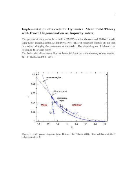
1Implementation of a code for Dynamical Mean Field Theorywith Exact Diagonalization as Impurity solverThe purpose of the exercise is to build a DMFT code for the one-band Hubbard modelusing Exact Diagonalization as impurity solver. The self-consistent solution should thenbe analyzed changing the parameters of the model. The phase diagram of reference canbe seen in the Figure below.The folder with all necessary files can be copied from the home directory of user cms00:cp -R ~cms00/ED_DMFT-2011 .Figure 1: QMC phase diagram (from Blümer PhD Thesis 2003). The half-bandwidth Dis here equal to 2.

2mini How-To1. The loop begins with file lisadiag.andpar containing, exactly as we did in Exercise2, the starting Anderson parameters (use just a, possibly educated, guess).2. As in Exercise 2, lisadiag.dat and lisadiag.input contain the other necessaryparameters.3. To get the impurity Green’s function on the Matsubara frequencies (iω n = iπT(2n+1)) at each iteration, the Anderson Impurity Model (AIM) code we worked withduring Exercise 2 can be used. It is also possible to use the version of lisadiag.fprovided here. The only thing to change is the definition of the frequencies: Nowthe Green’s function on the Matsubara axis is needed, instead of on real frequenciesas it was for Exercise 2. Either all or positive frequencies only, can be used. Thetwo places where this has to be done are marked by “?? Matsubara ??”.4. the solution of the AIM yields lisadiag.green containing G(iω n ).5. the DMFT self-consistency condition for the Bethe lattice case readsG 0 (iω n ) −1 = iω n + µ − D24 G(iω n)where D is the half-bandwidth. This equation can therefore be used to get the “new”G 0 (iω n ).IMPORTANT: This has to be written on the file G0w.dat, which is needed by theprogramfit.f. The format of such file is described below, as well as programfit.f.Additionally, to avoid possible oscillations between different solution during theDMFT loop, it would be desirable to mix the “new” G 0 (iω n ) - before writing itto the file G0w.dat - with, e.g., the non-interacting Green’s function of the AIM,namelyG And0 (iω n ) −1 = iω n + µ − ∑ kV 2kiω n − ǫ kAlternatively, the G 0 (iω n ) of the previous step can be used for the mixing.6. From the “new” G 0 (iω n ), the “new” Anderson parameters can be obtained througha fitting procedure. This can be done using the small program fit.f provided here.Program fit.f can be compiled in the following way:gfortran -fbounds-check -O fit.f -o FIT.x

3It looks into lisadiag.dat to initialize several arrays. Recompiling is necessaryevery time Ns and/or Iwmax are changed in file lisadiag.dat. The code alsoreads the Anderson parameters from lisadiag.andpar and the chemical potentialfrom lisadiag.input. These three files are expected to have the same format asthose used during Exercise 2 for the AIM code.7. As we already said, fit.f needs file G0w.dat to read G 0 (iω n ) from. This file has tocontain Iwmax (defined in lisadiag.dat) lines and three columns: The (real partof the) Matsubara frequency in the first column, and the real and imaginary part ofG 0 (iω n ) in the second and third columns.8. The output offit.f is a new set of Anderson parameters, contained in filenew.andpar.The format is the same as lisadiag.andpar, so simply copying new.andpar intolisadiag.andpar will be enough to start over with a new iteration.9. To check whether self-consistence has been reached, the AIM Green’s function G(iω n )can be plotted as a function of the iterations. When the changes in both the real andthe imaginary parts of G(iω n ) between to consecutive iterations are negligible, a selfconsistentsolution has been reached. A saturation in the values of the Andersonparameters as a function of the iteration also indicates that self-consistency hasbeen reached. More quantitative estimates of the convergece parameter would giveunambiguous results, but are not really needed in this context.Typically, of the order of 10-20 iterations are enough to converge, unless too fewAnderson parameters are used or unless there is a phase transition or a critical pointclose by. In those cases more iterations are needed, and the intial guess for theAnderson parameters becomes important.10. A consideration about the values of the Anderson parameters: These are determinedby a multi-dimensional fit of G 0 (iω n ) with the functional form G0 And (iω n ) −1 =iω n + µ − ∑ Vk2k iω n−ǫ k. This has no unique solution and since many regions of theparameter space can have shallow minima, tiny differences coming from roundingerrors can give different results for the final set of the Anderson parameters. Thismakes comparisons between different implentations of the self-consistency loop abit complicated. However, the values of the Anderson parameters have no physicalmeaning individually. Physical quantities like, e.g. the Green’s function, will dependmuch less on these small differences.