Time Variant Reliability Analysis of a Mobile Offshore Unit

THE SOCIETY OF NAVAL ARCHITECTS AND MARINE ENGINEERS“

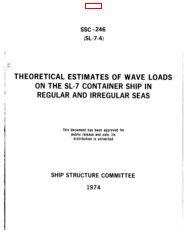
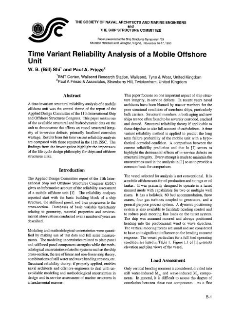
Ship Structures Symposium ’93approximation they may be considered independent. Recentdevelopments in probabilistic modeling of still waterand wave-induced loads on ships hulls are presented in[2], [3].Still Water LoadsThe shoti-term still water bending stress ~,Wof the vesselwas demonstrated in [4] to closely follow a Rayleighdistribution, see Figure 2.7 of [1] extracted horn [4],thereforeF(G,W)= 1 – e“”:’2B:~ (1)I Principle dimensionsIlLength between perpendiculars LPP 194.2 m IIfvlolded breadth Bm 32,0 m II Depth above baseline D 16.0 m IlDraught above baseline T 10.0 m II Draught above keel 12.0 I-n IDisplacement A 50620 tMidship section dataIfvlomertof inertiaabouthorizontal axis I, 180.5 m4 II Moment of inertia about vertical axis Iv474.5 m4 IlHeightof horiz.ne@mlaisakvebaseline 6.935 m ITable 1Principle dimensions and particularsFor the present analysis, a value of 19.44 MPa wasadopted for B,Was found in [4].Wave-InducedLoadsVerticaI and horizontal hull girder bending moments inregular waves were calculated-using linear s&ip theory [5].The hull form was modded with 28 unequally spacedsections. Two-dimensional hydrodynamic sectionalproperties were calculated with the Frank close-fit methodTransfer fanctions for combined stress response at theupper deck corner in forward and bow incoming waveswere calculated using the midship section moduli: 19,908m3 for vertical bending and 30.61 m3 for horizontal bending.In bow waves, the phase lag between vertical andhorizontal bending moments was taken into account. Thetransfer functions for combined stress, Figure 2.1 of [1],show that the highest stresses at an upper deck corneroccur when the waves encounter the ship from the oppositeside.If H, is significant wave height, T= is the mfian zeroup-crossing period, and co = wave frequency, the stressresponses in shofi-term irregular long-crested seas wereevaluated for the standard two-parameter Pierson-Moskowitzspectra according to[1 [1——H:T1 2n 5 -~~ ‘8n2 ~ Tze’ (2)‘W(w) =Non-1inear contributions due to changes in buoyancy,added mass and damping during the motion of the shipincrease the sagging bending moment by between 8 and18% whereas the hogging moment decreases by between15 and 17%. Assuming a symmetrical distribution aroundthe linear result, a bias factor of 1.15 for the saggingmoment and 0,85 for hogging seem appropriate for theextreme sea state. A standard deviation of 0.03 wasadopted to account approximately for the spread in theresults.For further load and strength analysis, only the verticalbending distribution obtained horn long-crested seas isapplied. This gives approximately 7% higher levels thanthe distribution for shoti-crested seas. Comparisons withfull scale measurements indicate a bias factor of 0.90 onthe calculated values for long-crested seas. It is reasonableto believe that the major part of the bias is due todirectional spreading.Hull Girder Cross”SectionalStrengthFor the cross-section reliabili~ analysis, a simplified approachwas chosen [7]. It is based on the observation thatthe ultimate moment capacity MUof longitudinally framedhulls under vertical bending is closely correlated to theultimate strength of the critical compression panel, asshown in Fig. 1 where MP is the fully effective plasticmoment. The hull girder ultimate strength model in [7] issummarized in Table 2.Analysis of the girder under hogging and sagging inaccordance with the Table 2 procedure was conducted.The results are listed in Table 3 from which it can be seenthat deck panel no. 3 is the most critical one from the girderstrength viewpoint although it is not tk panel demonstratingthe lowest panel strength.Failure Equationsand Probabilistic ModelingThe failure equation isX. W – XNLXMC z % – X,. Zqw>() (3)where MU is the ultimate bending moment evaluated asindicated in Table 2 and the remaining variables am asB-2

Shi and Frieze on ReliabilityAnalysis1“ Determine the plastic neutral axis position of the fully effective section, i.e. the axis that divides the section intotvvo patis with equal squash loads in compression and tension.>. . Calculate the plastic moment Mp.1. Identify the critical stiffened panel. As a first attempt, select the panel appearing most frequently in thecompression flange in either sagging or hogging. More precisely, calculate the cross-sectional strength for anumber of stiffened panels to identify that producing the lowest ultimate moment.LCompute values of the stiffened panel column slenderness A and the plate panel slenderness E!for the criticalpanel where1 = length of stiffened panelr = radius of gyration of fully effective stiffened panelL= (l/m) (oy/E)0.5 ~ = (b/t) (oY/E)0.5Gy = yield stress (use weighted average of plate and stiffener yield stress based on areas)E = Young’s modulusb = longitudinal stiffener spacingt = plating thickness?. Calculate the ultimate strength ratio q of the critical panelq = au/oy = (0.960 + 0.76512 -t 0.176~2 + 0.1 3112~2+ 1.046A4)+.5iCalculate the ultimate bending moment ratio for the girderin saggingMuS/MP = -0.172 + 1.548 q – 0.368 q2in hogging Muh/Mp = 0.003 + 1.459 q -0.461 T2Table 2Hull Girder Strength Model in Hogging and Saggingdefined in Table 4 together with their adopted distributionfunctions,The basis for the probabilistic modeling adopted for eachof the variables is as follows:- UY In this approach, the stiffened panel derivation considersadj scent half panels with altm-nate initial deformationmodes. Thus strength is controlled by the combinedfailing of the plate in one panel and the stiffener in theother. The stiffened panel response is initially governedby loss of stiffness in the initially distorted plating butstrength is then usually limited by the onset of yield at thestiffener tip. In [7] it was assumed in the derivation of thepresent formulation that the yield stresses in the plate andthe stiffener were the same. The effect of different yieldstresses has only been specifically examined in the courseof conducting comparisons between test results and predictions.An average value weighted in accordance withthe plate and stiffener areas was judged to be the mostappropriate value for the present analysis;- E,l,b,f,t~,dW,tW,tPmodeled as in the corresponding committeework of ISSC’88 [8];- UWbased on the linear long-crested wave bending resultsdeterminedabove;- O,Was determined above;- ~ this value maybe assessed by means of experimental-calculationcomparisons. This was conducted [71leading to a bias of 1.018 and COV of 0.061. The testsinvolved a small number of laboratory tests on steel boxgirders. These are not necessarily fully representative ofships girders so the COV was increased to 0.15, a compromisebetween the derived value and that of 0.20 suggestedin [9];- XNL ‘he ‘ffech ‘f ‘On-lineMib’ ‘ere ‘eScribed above.The bias found is in good agreement with that proposedin [10], namely, bias = 1.74- 0.93C~ where C~ is the blockcoet%cient - the agreement is acceptable considering thatthis equation was determined from scarce experimentaldata available on non-linem ship response. The standarddeviation adopted is also similar to that found in [10];- ZMCthis was evaluated from an analysis of the relevantfull scale data as described in [1]. The factor accounts forthe uncertainties arising from spectral representation andfrom the shape of the transfer function which is usuatlypredicted using linear strip theory. The model uncertainty,normally distributed with a bias of 0.90 and standarddeviation of 0.135, is in good agreement with theformulation in [10], namely,B-3

Ship Structures Symposium ’93PanelStfnr + r t bPlate(m)(mm)(m)@75Lb v MUIMP1 .088 18.5 0.810 .0391 0.523 1.711 0.731 0.7621 2 .087 17.5 0.850 .0391 0.529 1.900 0.702 0.733x o 3 .085 18.5 0.900 .0391 0.541 1.902 0.698 0.7298 *1,078 14.5 0.690 .0391 0.585 1.860 0.688 0.7183 1 .0795 13.5 0.690 .0391 0.579 1.990 0.679 0.7094 1 .0935 13.5 0.690 .0391 0.492 1.990 0.702 0.73311 .1399 10.5 0.725 .0391 0.329 2.700 0.640 0.7472 .1392 10.5 0.750 .0391 0.331 2.792 0.627 0.736E 2, .1387 10.5 0.670 .0391 0.332 2.494 0.668 0.772# s,md.1382 10.5 0.690 .0391 0.333 2.569 0.657 0.7621 .1382 10.5 0.690 .0391 0.333 2.569 0.657 0.7625 1 .1341 13.5 0.756 .0391 0.343 2.189 0.710 0.8066 1 .0680 18.0 0.500 .0391 0.677 1.086 0.743 0.8327 1 .1382 10.5 0.690 .0391 0.333 2.569 0.657 0.762Table 3Deck and Bottom Stiffened Panel Strength and Girder Ultimate Momentbias = –0,00506 + 0.42V + 0.70CP + 1.25 90°S 6 S 180°bias = –0.0063e + 1.22V + 0,66C~ + 0.06 OOS8 S 90°and a standard deviation is 0.12 where 0 is heading indegrees (180° corresponding to head waves) and V isFroude number. These equations have been determinedby a systematic comparison between theoretical and experimentalresults;- X,Wderived from the data in [4];- H,,TZ these were determined as the most likelihood fitsto the wave scatter diagram in [1], H, being based on a3-parameter Weibull distribution and TZ on a Iognormaldistribution;- a 0.1 mrd yr is a typical rate adopted by classificationsoci~ties although normally the COV can be expected tobe 100%, Vessels with inadequate maintenance whichresult in accelerated corrosion effects maybe declassed inrespect of ‘corrosion control’. in these cases, ratm apupreaching 0.2 mm/yr am more typical. The rate in thewebs and flange plates was taken as twice the basic valueadopted for the attached plating.ables R, and stochastic load processes Z(T). The variablesQ maybe the seastate parameters (e.g. significant waveheight and mean zero crossing period of, typically, threehours duration) and still water load affects the duration ofwhich is equal to that of the voyage. The R variablesinclude those describing material properties, corrosionrates, rnodding uncertainties of the limit state equationsand the statistical uncertainties of the seastate parameters.The processes Z(z) are the wave induced components.Figure 1 of[11] illustrates the durations of thww variousrandom variables.If the seastatesare assumed independent of each other, thelong tmrn probability Pf(t) can be expressed bywhere.“wP~(t)= 1 -(1 -Pm) E~~xj=l[k=l‘k‘Qk ~ ‘Qm{exp[-vi ‘Tk)A‘kj } (4)1]Time VariantReliabilityThe long term probability of the overall load effectsexceeding a degraded stiength threshold depends on randomparameters grouped into thrm categories, i.e. slowlyvarying random variables Q, time invariant random vari-v~j (~kj)Pm is the initial probabilityis the mean outcrossingdomain of the limit state equationinto its failure domain at the Tkjrate from the safeB-4

Shi and Frieze on ReliabilityAnalysisVariableDescriptionDistributionTypeMean ValueCovGy Yield stress Lognormal 392 0.066E Young’s modulus Normal 210,000 0.05I Panel length Normal 3700 0.04b Panel width Normal 690 0.04f Stiffener flange width Normal 90 0.04tf Flange thickness Normal 15 0.04dw Web height Normal 250 0.04t~ Web thickness Normal 10.0 0.04tp Plate thickness Normal 13.5 0.04Gw Wave bending stress N. process 0.0 Sea state dep.Osw Still water bending stress Rayleigh 24.36 0.523Xu Strength modulus uncertainty Normal 1.0 0.15‘NL Non-1inear correction Normal 1.15 0.026‘MCMeasured versus calculated Normal 0.90 0.15xSw Still water modulus uncertainty Normal 1.0 0.05H~ Significant wave height WeibullTZ Zero crossing period Lognormala Corrosion rate Logrtormal 0.1 -0.2 0.5- 1.0z Elastic section modulus Determ. 19.91.zP Plastic section modulus Determ. 28.00D Duration Determ. 0-20az Plastic section modulus reduction rate Lognormal 0.01-0.02 0.5- 1.0Stresses = MPa, dimensions=mm, corrosion rate= mm/yr, section modulus= m3, duration = yearTable 4Variable Probabilistic Modeling for Approach 1A ~kj k the time interwd of the~th seastat~ in the kthvoyagenk is the total number of sea states in thekfi voyagenvoy is the total number of voyages during theperiod (O,t)variables Q comprise the sea.state parameters Q,,, and thestill water load effects.Direct numerical calculation of the above equation is notfeasible, and it is always helpful to estimate the lower andupper bounds on P~(t) bypf(t) ~ P,I(t) = 1 – (1 – Pm) xQ,ea are the seastate parametersQkst are the still water load effects at thekti voyage.Normally, a marine unit undergoes several loading conditionssuch as homogeneously loaded, deep water ballast,etc. Variable Qkt belongs to the still water load effects ofone of these load conditions. For each load condition, the‘R ~ ‘Q, {exp [-~i ‘~ (t)] )[ 1Pf(t) s Pfi,(t) = 1 – (1 – Pl~) x(5a)(5b)B-5

Ship Structures Symposium ’93Pfu,(t) s P,.,(t) = 1 -(1tm- Pm);However, this equation becomes invalid when the longterm probability P~tiz(t)is high. In this case, the asymptoticLaplace integration technique gives poor estimates of P~(t)and even worse estimates of the sensitivity factors.whereyi is the mean percentagethe structure is in the iti’ loadcondition;of time during whichm is the total number of load conditions;Ni+(t) is the conditional mean outcrossing numberwithin a time period (O,t) in the itiload condition.Although eqns (6a) and (6b) can provide lower and upperbounds on P~(t), their calculation requires the solution tomulti-level integral problems. The scope of difficulty canbe envisaged.However, estimates of the lower and upper bounds on P~(t)can be calculated by using the asymptotic Laplace integrationtechnique. The theory is documented in manyreferences such as [12]. Its potential application to structuralreliability analysis is discussed in some detail in [13].What is more significant is that past asymptotic reliabilityanalysis methods are found to be related directly to andcan be explained by this technique.The concept of maximum likelihood can be more clearlyillustrated by application of the method. The lower andupper bounds to P~(t) require the following asymptoticresults.Estimation of PfU2(t) and its SensitivityFactorsThe solution of eqn (6c) can be easily obtained if the meanoutcrossing number E ~+Qy[Ni(t)] is known, Frequently,theg.meralized safety index is widely quoted tocompare relative structural safety. Following this convention,i3(t) denotes the safety index given byP(t) = -@-’ p,,,,(t) (6)[1The sensitivity factors of the estimated long-term probabilityof exceedance P~ti(t) to changes in distributionparameter values are also calculated based on the asymptoticLaplace integration technique. Hem the effects ofchanges in the distribution parameter @ orJ P*Uare notincluded because it is small compared with P~Uz(t).Thesensitivity factors are therefore given by!!l?-#=_9MLl m.m(t)] ,=1 ?“*](7)Estimationof PmThe initial probability Pm is relatively small comparedwith P~(t) and only gives an indication of the initial stressstate of the structure. If the random variables involved aredenoted as X = {R,Q,Z(~) } with a total number of randomvariables nx, the analytical expression of the initial probabilityPmiin the ith load condition isPm= ~ f, (x) dx = ~ exp[l,(x)]F’ Fwheredx , lX(X)= In f,(x)Fi is the integration domain at time ~ = O andcontains the area enclosed by thelimit state equation g(X,@

Shi and Frieze on ReliabilityAnalysisAX*is a nx x (nx - px) matrix the (nx - px)vectors of which form anorthonomal basis of the subspaceorthogonal to the subspacespanned by the px vectors in Ax.-Y (X,t)Tr(Y,t)F.(W).;E ~+~) i[N~ (t)] X ~y(12a)~1 ~ldet(A~A )[ ld.t[NTH N]lYY Y Y, Y~=1 ‘~The value of X* is obtained from the following minimisationmin -In fXi(X)for x ~ {g(X, ~)

Ship Structures Symposium ’93standard normal variables and curvature effects of the W denotes the transformed standard normallimit state equation are not considered. This solution is variables of R;f~,z (Q,Z) is the joint probabilitydensity function.The approximationto P~ti(t) in the end can be given as(15) Pti(t) = @ ( -IIW,UJI ) (18)whereA similar strategy can be adapted to determinePfl(t).I?n, Ozn are calculatedEstimationusing eqns (12c) and (12d) inthe transformed variable space;B is the distance from thE origin of thelmmsfonned variable space to th6most likely outcrossing point.of Pfl(t) and Pful(t)The lower and narrower upper bounds expressed by eqns(6a) and (6b) have to be determined by the nmted reliabilitymethod. The fundamental concept of this method iswell reported (14) (15) (16). So far, the nested reliabilitymethod based on FORM has normally been used &though, in principle, any reliability algorithm can be incorporatedat the expmse of having to determine higherorder derivatives. However, it should be noted that theaccuracy of the nested reliability method by FORM maybe undermined by the errors accumulated in a FORManalysis (17). A slightly different solution scheme hasbeen proposed in(18) based on a multiple objective minimisationstrategy. If P~Ul(t)is sought, the following formulationis required.Given a set of values of r ● R, it is always possible toestimate the conditional probability Pw(tlr). The unconditionalprobability Pti(t) is written hereafter asP,ti (t)= ~ P~u,(tlr)f

Shi and Frieze on ReliabilityAnalysisiterations required of nested reliability analyses. Thus, amajor computational advantage is realized with this technique.The most likely failure points for each of these casesassuming 20 years of exposure are listed in Table 5 togetherwith the 100 year result for Condition A. With the corrosionfree condition, generally only the time dependentvariables (bending stresses, wave height, etc) demonstratedifferent values at the most likely failure points. With theintroduction of corrosion, the failure point moves to adifferent part of the failure domain, the extent of the movedependimt upon the sensitivity of the system to the variableand, in turn, a function of its inherent variability. Thevariables most prominent in this respect are wave bendingstress, significant wave height, strength modeling uncertainty,and wave calculation accuracy,Comparison between the above corrosion h-m results andthe equivalent results presented in [1] demonstrates thatthey are in general agreement. Differences are to beexpected because of the different algorithms adopted toexecute the assessments.ConclusionThe effect of corrosion on the likelihood of ultimate girderfailure has been examined using a reliability procedurebased on the multiple objective minimisation technique.The example considered is the floating production unitanalyzed in some detail in the 1991 ISSC report by CommitteeV.I. However, as pointed out during the discussionat the Congress, the Committee report did not take accountof the effects of corrosion. It is hoped the presented workgoes some way to compensate for this.Condition (Service life)0:.- /$ A B c Da> (100 yr) (20 yr) (20 yr) (20 yr) (20 yr)@J 118.2 101.4 76.87 75.93 80.44Gsw 69.00 81.51 87.75 83.76 76,72H~ 12.97 12.16 11.00 10.85 11.21TZ 11.43 11.09 10.58 10.50 10.67Gy 379.1 379.1 385.3 389.3 390.4E 207800 207800 208600 209600 209800I 3707 3707 3710 3704 3702b 696.1 696.1 694.3 691.2 690.9f 89.90 89.90 89.94 89.98 89.98tf 14.98 14.98 14.98 15.00 15.00dw 248.8 248.8 249.3 249.8 249.9iw 9.999 9.999 9.998 9.999 9.999tp 13.40 13.40 13.42 13.48 13.49Xu 0.577 0.553 0.836 0.956 0.977‘NL 1.156 1.155 1.152 1.151 1.150‘MC 1.030 1.017 0.958 0.919 0.911x~w 1.009 1.011 1.007 1.002 1.001a 0.1050 0.0787 0.1966C& 0.0166 0.0235 0.0196-..— Table 5Values of the Basic Variables atthe Most Likely Failure Point1.2.3.4.5.6.7.8.9.ReferencesReport of Committee V. I., “Applied Design,” Proceedingsof the 1lth International Ship and OffshoreStructures Congress, Volume 2, Edited byP.H. Hsu and Y.S. Wu, Elsevier Applied Science,London 1991.Guedes Soares, and Moan, Trans. Society of NavalArch. and Marine Engineers, Vol. 96,1988, pp.129-156.Guedes Soares, Structural Safety, Vol. 8,1990, pp.353-368.Moan, T. and Jiao, G., “Characteristic Still Water Effectsfor Production Ships;’ University of Trondheim,December 1988.Salvesen, Tuck and Faltinsen, SNAME Transactions,Vol 78, 1970.Frank, W., “Oscillation of Cylinders in or Below theFree Surface of Des;’ NSRDC Report 2375, 1967.Frieze, P,A. and Lin, Y-T,, “Ship LongitudinalStrength Modeling for Reliability Analysis:’ ProceedingsMarine Structural Inspection, Maintenanceand Monitoring Symposuim, SSCISNAME,Arlington, March 1991.Report of Committee V. I., “Applied Design,” Proceedings,10th International Ship and OffshoreStructures Congress, Vol. 2, Technical Universi~of Denmark, Lyngby, 1988.Faulkner, D., oral discussion to Report of ISSC’88Committee V. 1, Lyngby, August, 1988B-9

Ship Structures Symposium ’9310.Gwsdes Soares, C. and Moan, T., “UncertaintyAnalysis and Code Calibration on the primaryLoad Effects in Ship Structures;’ ICOSSAR ’85,4th International Conference on Structural Safetyand Reliability, 1985.11. Shi, W.B., “Load Combinations by Log-LikelihoodMaximization;’ in Practical Design of Ships andMobile Units, Edit~d by J.B. Caldwell and G.Ward, Elsevier Applied Science, London, Vol 2,pp. 2.953-2.965.14.15.16.Madsen and Tvedt, J. of Eng. Mech., Vol. 116, No.10,1990.Fujita, M., Schall, G. and Rackwitz, R., “Time VariantComponent Reliabilities by FORM/SORM andUpdating by Importance Sampling,” Proceedings5th International Conference on Appl. of Statisticsand Probability in Civil Engineering, Vancover,1987.Wen and Chen, Prob. Eng, Mech., Vol. 2, 1987, pp.156-162.12.13.Bleinstein, N. and HandeJsman, R., “Asymptotic Expansionsof Integrals,” Dover, New York, 1986.Breitang, J. of Eng. Mech., Vol. 117, No. 3,1991.17.18.Ronold, J. of Eng. Mech., Vol. 117, No. 9, 1991.Shi, Marine Structures, Vol. 4, No. 5, 1991, pp. 435-453.B-10

Shi and Frieze on ReliabilityAnalysis11MdMFMm0.80.80.60.60.4●metfitCulveNumerical values0.4●Eastflt curveNumerbxlvalues0.20.$?0.4 i.6 0.8 1 64 0.6 0.8 1Criticalstiffmd panel strength Critical stiffened panel strength(a) Hull in Sagging(b) Hull in HoggingFigure 1Ultimate Bending Moment versus Critical Panel Strength4Reliabilityindex-.Condltbn A=.